Abstract
Forest fires create burned and unburned areas on a spatial scale, with the boundary between these areas known as the fire boundary. Following an analysis of forest fire boundaries in the northern region of Yangyuan County, located in the Liangshan Yi Autonomous Prefecture of Sichuan Province, China, several key factors influencing the formation of fire boundaries were identified. These factors include the topography, vegetation, climate, and human activity. To explore the impact of these factors in different spaces on potential results, we varied the distances between matched sample points and built six fire environment models with different sampling distances. We constructed a matched case-control conditional light gradient boosting machine (MCC CLightGBM) to model these environment models and analyzed the factors influencing fire boundary formation and the spatial locations of the predicted boundaries. Our results show that the MCC CLightGBM model performs better when points on the selected boundaries are paired with points within the burned areas, specifically between 120 m and 480 m away from the boundaries. By using the MCC CLightGBM model to predict the probability of boundary formation under six environmental models at different distances, we found that fire boundaries are most likely to form near roads and populated areas. Boundary formation is also influenced by areas with significant topographic relief. It should be noted explicitly that this conclusion is only applicable to this study region and has not been validated for other different regions. Finally, the matched case-control conditional random forest (MCC CRF) model was constructed for comparison experiments. The MCC CLightGBM model demonstrates potential in predicting fire boundaries and fills a gap in research on fire boundary predictions in this area which can be useful in future forest fire management, allowing for a quick and intuitive assessment of where a fire has stopped.
1. Introduction
Forests are a crucial ecological resource. However, fire, which is one of the primary threats to forests, poses a significant danger to both forest ecosystems and human life and property [1,2,3]. To manage forests effectively and establish safe areas after a fire, it is essential to have information about where a fire is likely to stop. This cessation can be influenced by the fire environment just as the fire’s spread can be [4]. In situations where there is insufficient fuel or high moisture content in the topography and vegetation [5], the fire intensity will gradually diminish and eventually stop because it cannot generate enough heat to keep the fire alight [6]. The transition zone between the burned and unburned areas is the fire boundary [7].
With the continuous advancement of artificial intelligence technologies, their applications in academic research have become increasingly extensive. In particular, machine learning and deep learning methodologies have demonstrated exceptional performances across numerous research domains. These domains include, but are not limited to, natural language processing, computer vision, bioinformatics, and predictive modeling. The essence of these methodologies lies in their ability to learn and extract valuable information from vast amounts of data, thereby enabling the understanding and prediction of complex systems. For instance, in the field of material science, researchers have used deep learning methods to predict the resilient modulus of modified base materials subjected to wet–dry cycles [8]. In the domain of forest fire prediction, Tehrany Mahyat Shafapour et al. employed a LogitBoost machine learning classifier and multi-source geospatial data to spatially predict the susceptibility to tropical forest fires [9]. In the study of Cuesta et al. [10] which analyzed the factors that influence the formation of unburned areas, it was indicated that topographic, climatic, and vegetation factors can play a key role in the fire intensity and spread rate which are the main factors that influence the formation of unburned areas. In a fire cessation analysis model, Kiera A.P. Macauley et al. modeled fire cessation based on topographic, climatic, vegetation, and human activity factors [11]. The results showed that the vegetation type has a strong influence on fire cessation. In fire cessation studies conducted in the western United States, fires tended to stop in valleys or near roads, while in mountainous environments, the topography had the greatest effect on fire cessation [12]. In a forest fire spread model proposed by Zechuan Wu et al. based on neural networks, the most important factors that affect the spread of forest fires in Heilongjiang are altitude and temperature while wind speed and direction are more influential than precipitation [13]. N. Ryzhkova et al. reconstructed the 600-year fire history of a mid-boreal and pine-dominated landscape in the southern Republic of Komi, Russia, using dendrochronology. The fire activity cycle is influenced by both the climate and human land use but is primarily controlled by the climate. The association between the establishment of villages and occurrence of fires is not significant, whereras the correlation with historical drought conditions is more so pronounced [14]. However, these studies on fire cessation have statistically analyzed the environment and fire conditions of the entire study area without considering matching data at different distances from the burned and unburned areas on a spatial scale to better analyze the complexity and diversity of the fire environment [15]. As a result, the analysis of the factors influencing fire cessation is limited and the accuracy of predicting the location of fire cessation may be affected [16].
In this study, we analyzed the effect of the fire environment on fire cessation in the northern forest area of Yangyuan County, Liangshan Yi Autonomous Prefecture, Sichuan. To our knowledge, there is no corresponding research on fire boundaries in this area. To do so, we selected topographic, climatic, vegetation, and human activity factors at different distances along the fire boundaries in burned and unburned areas. We then assessed the relationship between the burned and unburned areas and analyzed the influence of various fire factors upon fire cessation.
Previous studies have ignored the spatial variability of fire environments and did not perform matched controls of fire environments [17,18,19]. Therefore, we constructed the matched case-control conditional light gradient boosting machine (MCC CLightGBM) to predict the probability of fire boundary formation at different distances from the fire environment and to give the importance of the factors influencing fire boundary formation in the study area by choosing the optimal model. We evaluated the area under the curve (AUC), F1-score, and accuracy (ACC) of each model [20,21]. These are useful indicators of the closeness of the predicted and actual fire occurrence in the study area (burned area, unburned area, and boundaries). Finally, the matched case control conditional random forest (MCC CRF) was constructed for comparison experiments.
The analysis and prediction of fire environments and boundaries will allow forest managers in the study area to better establish fire safety zones, which will have a beneficial impact on forest protection and firefighting efforts. However, the reference value for other regions still needs to be verified.
2. Materials and Methods
2.1. Study Area
The study area is a forested region located in northern Yangyuan County, Liangshan Yi Autonomous Prefecture, Sichuan Province, with the Yalong River running through the entire area (see Figure 1). It has an elevation range of 1636 m to 4369 m and covers a total area of 301.1 km. The area is dominated by evergreen broadleaf forests in the east Sichuan basin and southwest Sichuan mountains and coniferous forests in the west Sichuan alpine valley mountains, with a forest cover of 80%. The region has a subtropical monsoon climate characterized by abundant sunshine and rainfall, with an average annual temperature of 16.7 and an annual rainfall of 1450 mm.
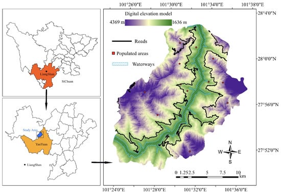
Figure 1.
The study area located in Liangshan, Sichuan, China.
2.2. Sampling Design and Dataset
Based on relevant studies and the size of the sampling raster in the study area [22], we collected one sample every 180 m along the fire boundary and created a digital linear strip perpendicular to the fire boundary for each sample using ArcGIS. The linear strips were sampled at distances of 30 m, 120 m, 180 m, 240 m, 300 m, 360 m, 420 m, and 480 m in the burned and unburned areas, respectively (see Figure 2). The points on each sample strip were manually checked to remove any points that did not correspond to the burned or unburned state. For example, if the length of a strip in the burned area was less than 480 m, the point taken at 480 m would be unburned and not match the state on the sample strip and therefore needed to be removed. Given the diversity and complexity of fire environments, we have divided fire environments into six fire environment models according to different sampling distances. These models use data points collected from various distances from the fire boundary, both within the burned and unburned areas.
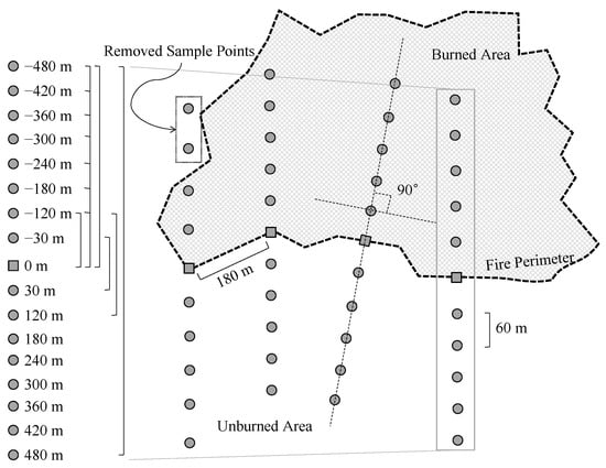
Figure 2.
Sampling methodology for the stable and dynamic fire environment models.
- The ’Case 0 m, Control −120 m Model’ uses data points at the fire boundary (0 m) as case data and data points 120 m within the burned area from the fire boundary as control data;
- The ’Case 0 m, Control −120 m∼−480 m Model’ employs data points at the fire boundary as case data and data points ranging from 120 m to 480 m within the burned area from the fire boundary as control data;
- The ’Case 0 m, Control −480 m Model’ utilizes data points at the fire boundary as case data and data points 480 m within the burned area from the fire boundary as control data;
- The ’Case 30 m, Control −30 m Model’ uses data points 30 m within the unburned area from the fire boundary as case data and data points 30 m within the burned area from the fire boundary as control data;
- The ’Case 120 m, Control −120 m Model’ employs data points 120 m within the unburned area from the fire boundary as case data and data points 120 m within the burned area from the fire boundary as control data;
- The ’Case 480 m, Control −480 m Model’ utilizes data points 480 m within the unburned area from the fire boundary as case data and data points 480 m within the burned area from the fire boundary as control data.
Based on the literature related to fire spread and burned area formation, we collected factors influencing the formation of the potential fire boundary, including topographic, climatic, vegetation, and human activity factors, which can well describe the fire environment at the sample sites [23,24,25]. In this study, climatic factors include the temperature (TMP), wind speed (WS), water vapor pressure (WVP), and precipitation. TMP can indicate the potential for water evaporation in the environment, where the higher the value, the easier the water evaporates, and the drier the air, which is conducive to fire growth [26]. When the value of WVP is higher, it usually means that the air is more humid [27]. Changes in the WS can affect the velocity of air flow, resulting in variations in the air and soil temperature as well as the humidity [28]; WS can also influence the direction and morphology of plant growth [29]. Precipitation directly impacts the intensity of the fire, where rainfall can increase soil and vegetation moisture and slow down the fire burning process; if heavy enough, it may completely stop the spread of fire [30]. Considering the fact that climatic conditions are dynamic and variable throughout the month, we used the monthly average observations [31].
We included five topographic factors as potential influencing variables in our study. Altitude affects vegetation growth and the atmospheric temperature, humidity, and oxygen content, leading to variation in fire conditions [32]. The aspect of a slope can affect humidity and the dryness of combustible materials, making fire spread uphill more likely due to both convection and heat transfer [33]. The topographic wetness index (TWI) indicates the spatial distribution of soil moisture in watersheds which affects fire occurrence and spread [34]. The slope, aspect, and altitude can all affect water evaporation and the slope steepness can influence the direct contact of flame with fuel sources [35]. We also measured the distance from the sampling site to the nearest waterways as rivers may act as natural fire boundaries.
The vegetation growth distribution, coverage, and the context of the vegetation canopy are all factors that can influence the fuel of a fire [36]. The distribution of vegetation is reflected in the normalized difference vegetation index (NDVI) [37].
Human activity, such as the careless disposal of cigarette ends near roads or human settlements, can trigger accidental fires [38]. These fires typically stop near roads and form boundaries so it is important to consider human activity factors, such as the distance to roads (DTR) and the distance to populated areas (DTP) [35].
To investigate the fire environment inside and outside the fire boundaries at each sample point, the study area was converted into a 30 × 30 m raster using ArcGIS. The corresponding influence factor data and monthly fire points for the high fire months (2020–2022) were extracted using products such as Landsat-8, the Moderate Resolution Imaging Spectrometer (MODIS), and the 30 m Digital Elevation Model (DEM). The spatial distribution of each influencing factor is illustrated in Figure 3. The fire conditions on and outside the fire boundary (unburned area) are denoted as 0 while the conditions inside the boundary (burned area) are denoted as 1. The area of the burned area is 30 km and the individual values are mapped to each raster. Table 1 provides the specific details about the influencing factors and the range of the dataset for the study area.
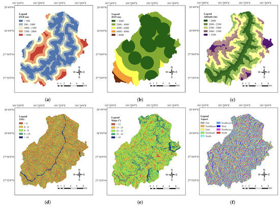
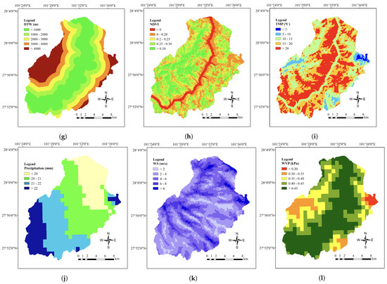
Figure 3.
The spatial distribution of fire boundary-influencing factors: (a) DTR. (b) DTP. (c) Altitude. (d) TWI. (e) Slope. (f) Aspect. (g) DTW. (h) NDVI. (i) TMP. (j) Precipitation. (k) WS. (l) WVP.

Table 1.
Classification of the influencing factors.
2.3. Statistical Modelling
To investigate the relationship between the fire environment and fire boundary formation, we applied the MCC CLightGBM model to the study area. This approach integrates the matched case-control study [39], which is commonly used in pathology, with the machine learning LightGBM model. We selected samples from the fire boundaries and unburned areas as the case group and samples from the burned areas as the control group. We employed the MCC CLightGBM method to examine whether the fire environment factors are associated with fire boundary formation, quantify the strength of this association, and predict the probability of fire boundary formation at different distances from the fire environment. We also used the MCC CRF method for comparison to evaluate the performance of the models.
Previous studies modeling fire cessation have compared burned and unburned locations at a spatial scale. This scale is chosen to be close enough to observe fire behavior processes, yet distant enough to ensure that distinct states are seen on each side of the fire edge [40]. These models are typically accomplished by predefining the spatial extent or span of the fire boundaries and subjectively setting the proximity between burned and unburned observation points [41]. However, to date, no investigations have specifically addressed how the distance between case and control sample points influences conclusions about fire environment processes on fire cessation. To assess the sensitivity of our results to subjective decisions about the proximity of matched burned and unburned sample points [42], we varied the distance between paired points and developed six spatial-scale models based on topographic, vegetation, climatic, and human activity variables (see Figure 2). Cases on the fire boundaries (i.e., 0 m) were paired with samples at 120 m, 480 m, and all samples between them within the burn area, using two pairs of samples at 30 m, 120 m, and 480 m inside and outside the fire boundaries. Given that the raster resolution is 30 × 30 m, the minimum sampling distance is 30 m. We combined significant variables into a final predictive model to assess the stable fire environment’s influence on fire cessation.
Before modeling, we evaluated multicollinearity between the variables using the Variance Inflation Factor (VIF) and removed variables with VIF values greater than 5. We verified the importance of each influencing factor on the formation of fire boundaries using Spearman’s Rank Correlation Coefficient (SCC) [43]. Finally, we validated the prediction model performance using evaluation metrics such as the Area Under the Curve (AUC), F1-score, and Accuracy (ACC).
To obtain the fire boundary prediction model with the highest accuracy, evaluation metrics such as the AUC, F1-score, and ACC were used to compare the performance of different models. The model with the highest prediction accuracy was selected as the final fire boundary prediction model. The probability of fire boundary formation in the study area was compared to the actual fire boundaries to provide forest managers with a theoretical basis for avoiding risks and establishing safe havens. Figure 4 illustrates the general workflow from the data input to obtaining the fire boundary maps.
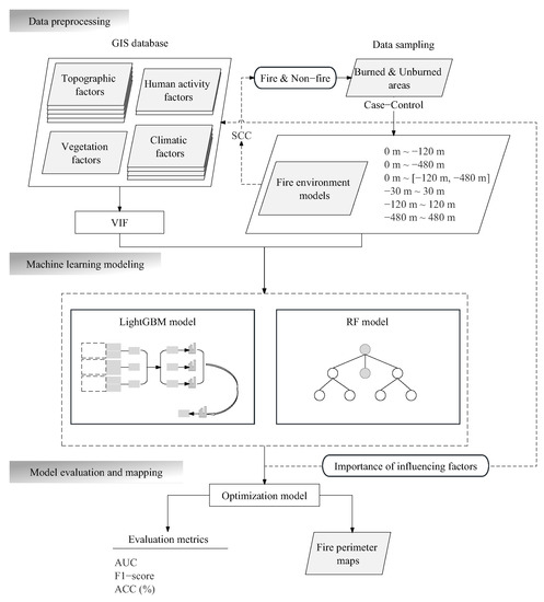
Figure 4.
The general workflow shows the interaction from data input to the produced fire perimeter maps.
3. Results
The VIF analysis was conducted for all six models and variables with VIF values greater than five were excluded. The results of the input variables for each model are presented in Table 2. Only two models (case 0 m, control −480 m and case 480 m, control −480 m) required the removal of variables. The standard error (S.E.) is presented in Table 2 and the p-value indicates a significant correlation between the variable and formation of fire boundaries. The p-value < 0.05 indicates a significant correlation and the variable can be used for modeling.
Table 2.
Fire environment model results for different sampling distances.
Spearman’s rank correlation coefficient (SCC) analysis of the influencing factors in the combined six models (Figure 5a) revealed that DTR and DTP had the most significant influence on fire boundary formation which is consistent with actual observations. Fires that spread near roads or populated areas which may be disturbed by buildings and human activity will stop and form boundaries. The effect of precipitation on fire boundary formation was not significant due to the low rainfall in the month when fires occurred in the study area.
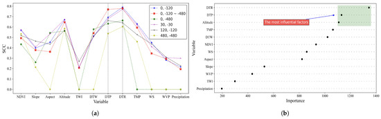
Figure 5.
The importance of fire boundary-influencing factors: (a) The SCC change curves for six environment models. (b) The importance of variables.
The MCC CLightGBM model was constructed to predict fire boundaries for six environmental models with different sampling distances and actual fire boundary maps were superimposed. These maps were compared with the actual fire boundaries to provide a theoretical basis for forest managers to avoid risks and establish safe havens.
The dataset is randomly divided into 70% for training and 30% for testing. Subsequently, six environmental models are trained using the MCC CLightGBM and MCC CRF methods, respectively. The results are presented in Table 2. As the distance between the matched case and control pairs increased from 120 m to 480 m, the model’s predictive ability also increased (i.e., for MCC CLightGBM: AUC of 0.86 and 0.88, F1-score of 0.78 and 0.73, and ACC of 81.83% and 84.87%, respectively. The trend of MCC CRF results was also similar). When the distance between matching pairs was increased to 60 m, 240 m, and 960 m, the model prediction accuracy also increased (i.e., MCC CLightGBM achieved an accuracy of 83.49%, 84.36%, and 84.75%, respectively, while MCC CRF achieved an accuracy of 82.35%, 83.44%, and 84.87%, respectively). Among the six different sampling models, the model with the highest prediction accuracy was that with case 0 m and control −120 m to −480 m, where MCC CLightGBM and MCC CRF achieved accuracies of 87.86% and 84.93%, respectively. Figure 6 illustrates that the histogram distributions of both training and testing data for the optimal environmental model align closely. This consistency contributes to an enhanced performance of the boundary prediction model, enabling it to handle a broader range of data from diverse fire environments.
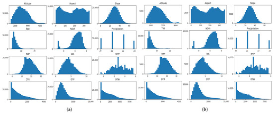
Figure 6.
Histogram distribution: (a) Histogram distribution of training data. (b) Histogram distribution of test data.
Based on the results of six environmental models with varying sampling distances and two prediction models (see Figure 7), it is evident that the MCC CLightGBM prediction model in the Case 0 m, Control −120 m∼−480 m model performs the best. The importance ranking of each influencing factor in this model is shown in Figure 5b, with DTR and DTP identified as having the greatest impact on fire boundary formation, which is consistent with the SCC analysis depicted in Figure 5a. The probabilities of fire boundary formation in the study area and the actual fire boundaries are shown in Figure 8. As can be seen in the figure, the MCC CLightGBM prediction model predicts a clear and more refined delineation of the probability of fire boundary formation in the Case 0 m, Control −120 m∼−480 m environment model. Combined with the topographical map in Figure 3, it can be seen that in areas with human settlements and roads the fire boundaries tend to coincide with these features, serving as natural fire boundaries. Although rivers can serve as natural fire boundaries in nature, their effect on boundary formation is not prominent in this study area due to the presence of roads near the waterways, with the fires stopping near these roads.
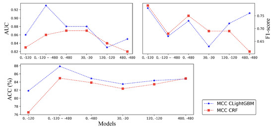
Figure 7.
The performance of two prediction models on different sampling distance models.
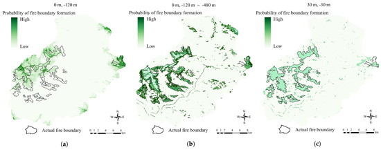
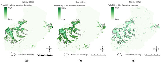
Figure 8.
Fire boundary formation probability map for the study area: (a) Case 0 m, Control −120 m. (b) Case 0 m, Control −120 m∼−480 m. (c) Case 30 m, Control −30 m. (d) Case 120 m, Control −120 m. (e) Case 0 m, Control −480 m. (f) Case 480 m, Control −480 m.
4. Discussion
4.1. Fire Environment Influence
When analyzing the influence of the fire environment on fire boundary formation, we considered topographic, vegetation, climatic, and human activity factors. The results from different sampling distance models show that the distance to roads and populated areas strongly influences the formation of forest fire boundaries in the region. These areas are dominated by cemented areas with sparse vegetation and high human activity where fires can easily stop. Altitude also has a significant influence to some extent. As fires spread to higher elevations, they require more thrust and heat [44], so boundaries may also form at places with large changes in elevation or slope [45], such as at the foot of mountains (see Figure 8). The study shows that sparse vegetation has a positive effect on fire boundary formation [46] and the fires in this study area are concentrated in the west where vegetation is more evenly distributed; only areas near roads and waterways have less vegetation (see Figure 3h). Therefore, the effect of vegetation on fire stopping is not as significant as the effect of the distance to roads and waterways. Since there is little spatial variation in the climate during fires in the region and no severe weather (see Figure 3i–l), the influence of the climate on the formation of fire boundaries is not significant.
4.2. Influence of the Sampling Distance on Model Performance
To improve the accuracy and reliability of the model, we took into account the variability of individual variables by considering different sampling distances. The models were divided into six categories based on the sampling distance, with the minimum distance being 30 m, which is the minimum distance of the raster; the farthest distance being 480 m. This distance allows for significant variability in the variables without using fire point data that do not match the actual burned conditions. The prediction model that utilized matched pairs located at 0 m and −120 m∼−480 m distances from the digital fire boundary performed the best overall, with an acceptable accuracy, AUC, and F1-score. It is possible that the larger amount of data and effective reflection of the difference between the fire environment in the burned and unburned areas in this set of sampling distance models contributed to better training of the prediction model. As the variability of the fire environment increases at the spatial scale, the prediction accuracy of the model improves as the distance between the case and control pairs expands (Figure 7).
4.3. Fire Boundary Prediction Model
To select a fire boundary prediction model for the study area, we analyzed six different sampling distance models and compared the MCC CLightGBM and MCC CRF models. The MCC CLightGBM model was chosen as the prediction model. Of the six environmental models, the Case 0 m, Control −120 m∼−480 m model is optimal because its delineated fire boundaries form a clearer and more accurate probability map. In contrast, in the fire boundary fractal model proposed by RS McAlpine et al., the predicted fire boundaries are very coarse, with artificially delineated polygons as boundaries and the accuracy is low [47]. The MCC CLightGBM model proposed in this paper can greatly improve the prediction accuracy and speed of forest fire boundaries.
From the model results, it can be observed that fires tend to stop near roads and populated areas and in areas with significant altitude changes such as valleys. Fires also tend to stop spreading near waterways but in this study area, the effect of waterways on fire boundary formation is limited due to the distribution of roads on both sides of the waterways.
5. Conclusions
The hybrid models MCC CLightGBM and MCC CRF have demonstrated advantages in predicting forest fire boundaries based on the analysis of common model evaluation metrics, with the MCC CLightGBM model achieving higher prediction accuracy. Our analysis also shows that topographic, climatic, vegetation, and human activity factors all have an influence on fire cessation, with the distance to roads, distance to populated areas, and altitude having the greatest influence on the formation of fire boundaries. Precipitation had the least effect on fire cessation as the area received very little rainfall in the month when the fire occurred. Among the six models with different sampling distances, the Case 0 m, Control −120 m∼−480 m model performed the best. Based on the predicted probability of fire boundary formation and the actual boundary maps, it can be seen that in general, fires in the study area tend to stop near roads, populated areas, and valleys. Therefore, fires are more likely to occur and spread easily in areas with high vegetation and low human activity. Areas located beyond the fire perimeter are comparatively safer, allowing forest management personnel to establish refuge points in these regions. Conversely, within the fire boundary, the likelihood of fire cessation diminishes significantly, necessitating immediate deployment of firefighters to these areas to effectively suppress the fire. It should be noted explicitly that this conclusion is only applicable to this study region and has not been validated for other different regions. Moreover, the use of a combination of a matched case-control study commonly used in medicine and the novel LightGBM machine learning approach not only improves model prediction performance but also considers the impact of spatial variability in the fire environment on model performance. This study fills a gap in the research on fire boundary predictions in this area, offering a theoretical basis for local forest management personnel in planning facilities such as fire shelters and lookout towers.
Author Contributions
The four authors contributed equally to each and every stage of this research work. All authors have read and agreed to the published version of the manuscript.
Funding
This work was supported in part by the Start-up Fund for New Talented Researchers of Nanjing Vocational University of Industry Technology (Grant No. YK22-05-01) and the Open Foundation of Industrial Software Engineering Technology Research and Development Center of Jiangsu Education Department (ZK20-04-05).
Data Availability Statement
A 30 m-resolution DEM data can be downloaded from Geospatial Data Cloud (GDC) (https://www.gscloud.cn, accessed on 4 June 2023). The MODIS data can be downloaded from National Aeronautics and Space Administration (NASA) (https://ladsweb.modaps.eosdis.nasa.gov/, accessed on 4 June 2023).
Conflicts of Interest
The authors declare no conflict of interest.
Abbreviations
The following abbreviations are used in this manuscript:
| MCC CLightGBM | Matched case-control conditional light gradient boosting machine |
| MCC CRF | Matched case-control conditional random forest |
| TMP | Temperature |
| WS | Wind speed |
| WVP | Water vapor pressure |
| TWI | Topographic wetness index |
| NDVI | Normalized difference vegetation index |
| DTR | Distance to roads |
| DTP | Distance to populated areas |
| DTW | Distance to waterways |
| MODIS | Moderate resolution imaging spectrometer |
| DEM | Digital elevation model |
| VIF | Variance inflation factor |
| SCC | Spearman’s rank correlation coefficient |
| AUC | Area under the curve |
| ACC | Accuracy |
| S.E. | Standard error |
References
- Liu, H.; Xu, X. Exploring the ‘dark’ side of forest therapy and recreation: A critical review and future directions. Renew. Sustain. Energy Rev. 2023, 183, 113480. [Google Scholar] [CrossRef]
- Lin, J.; Lin, H.; Wang, F. A Semi-Supervised Method for Real-Time Forest Fire Detection Algorithm Based on Adaptively Spatial Feature Fusion. Forests 2023, 14, 361. [Google Scholar] [CrossRef]
- Barmpoutis, P.; Kastridis, A. Suburban Forest Fire Risk Assessment and Forest Surveillance Using 360-Degree Cameras and a Multiscale Deformable Transformer. Remote Sens. 2023, 15, 1995. [Google Scholar] [CrossRef]
- Liu, X.; Tong, Z. Uncertainty simulation of large-scale discrete grassland fire spread based on Monte Carlo. Fire Saf. J. 2023, 135, 103713. [Google Scholar] [CrossRef]
- Nur, A.; Kim, Y.; Lee, J. Spatial Prediction of Wildfire Susceptibility Using Hybrid Machine Learning Models Based on Support Vector Regression in Sydney, Australia. Remote Sens. 2023, 15, 760. [Google Scholar] [CrossRef]
- Zhang, Z.; Tan, Y.; Hong, R.; Zhao, Y.; Zhang, H.; Zhang, Y.; Li, Z. Experimental investigation of tunnel temperature field and smoke spread under the influence of a slow moving train with a fire in the carriage. Tunn. Undergr. Space Technol. 2023, 131, 104844. [Google Scholar] [CrossRef]
- Culler, E.; Livneh, B. A data-driven evaluation of post-fire landslide susceptibility. Nat. Hazards Earth Syst. Sci. 2023, 23, 1631–1652. [Google Scholar] [CrossRef]
- Esmaeili-Falak, M.; Benemaran, R. Ensemble deep learning-based models to predict the resilient modulus of modified base materials subjected to wet-dry cycles. Geomech. Eng. 2023, 32, 583–600. [Google Scholar]
- Tehrany, M.; Jones, S. A novel ensemble modeling approach for the spatial prediction of tropical forest fire susceptibility using LogitBoost machine learning classifier and multi-source geospatial data. Theor. Appl. Climatol. 2019, 1, 637–653. [Google Scholar] [CrossRef]
- Cuesta, R.; Gracia, M.; Retana, J. Factors influencing the formation of unburned forest islands within the perimeter of a large forest fire. For. Ecol. Manag. 2009, 258, 71–80. [Google Scholar] [CrossRef]
- Macauley, K. Modelling Fire Cessation in the Canadian Rocky Mountains. Master’s Thesis, University of Alberta, Edmonton, AB, Canada, 2020. [Google Scholar]
- Nicholas, A.; Paul, F.; Brion, R.; Retana, J. Evidence for scale-dependent topographic controls on wildfire spread. Ecosphere 2018, 9, e02443. [Google Scholar]
- Wu, Z.; Wang, B.; Li, M.; Tian, Y.; Quan, Y.; Liu, J. Simulation of forest fire spread based on artificial intelligence. Ecol. Indic. 2022, 136, 108653. [Google Scholar] [CrossRef]
- Ryzhkova, N.; Kryshen, A.; Niklasson, M.; Pinto, G. Climate drove the fire cycle and humans influenced fire occurrence in the East European boreal forest. Ecol. Monogr. 2022, 92, e1530. [Google Scholar] [CrossRef]
- Kolden, C.; Lutz, J.; Key, C. Mapped versus actual burned area within wildfire perimeters: Characterizing the unburned. For. Ecol. Manag. 2012, 286, 38–47. [Google Scholar] [CrossRef]
- Christopher, D.; David, E.; Matthew, P. An empirical machine learning method for predicting potential fire control locations for pre-fire planning and operational fire management. Int. J. Wildland Fire 2017, 26, 587–597. [Google Scholar]
- Cliff, H.; Catt, G.; Holmes, J. Right-way fire in Australia’s spinifex deserts: An approach for measuring management success when fire activity varies substantially through space and time. J. Environ. Manag. 2023, 331, 117234. [Google Scholar]
- Fabi, A.; Thampi, S. A trust management framework using forest fire model to propagate emergency messages in the Internet of Vehicles (IoV). Veh. Commun. 2022, 33, 100404. [Google Scholar] [CrossRef]
- Lin, H.; Tang, C. Analysis and optimization of urban public transport lines based on multiobjective adaptive particle swarm optimization. IEEE Trans. Intell. Transp. Syst. 2021, 23, 16786–16798. [Google Scholar] [CrossRef]
- Jeong, M. Grid-based Urban Fire Prediction Using Extreme Gradient Boosting (XGBoost). Sens. Mater. 2022, 34, 4879–4890. [Google Scholar]
- Dong, H.; Wu, H.; Sun, P.; Ding, Y. Wildfire Prediction Model Based on Spatial and Temporal Characteristics: A Case Study of a Wildfire in Portugal’s Montesinho Natural Park. Sustainability 2022, 14, 10107. [Google Scholar] [CrossRef]
- Macauley, K.; McLoughlin, N.; Beverly, J. Modelling fire perimeter formation in the Canadian Rocky Mountains. For. Ecol. Manag. 2022, 506, 119958. [Google Scholar] [CrossRef]
- Coop, J.; Parks, S.; Stevens-Rumann, C.; Ritter, S.; Hoffman, C. Extreme fire spread events and area burned under recent and future climate in the western USA. Glob. Ecol. Biogeogr. 2022, 31, 1949–1959. [Google Scholar] [CrossRef]
- Lei, M.; Cui, Y.; Ni, J.; Zhang, G.; Li, Y.; Wang, H.; Liu, D.; Yi, S.; Jin, W.; Zhou, L. Temporal evolution of the hydromechanical properties of soil-root systems in a forest fire in China. Sci. Total Environ. 2022, 809, 151165. [Google Scholar] [CrossRef]
- Cui, L.; Luo, C.; Yao, C.; Zou, Z.; Wu, G.; Li, Q.; Wang, X. The influence of climate change on forest fires in Yunnan province, Southwest China detected by GRACE satellites. Remote Sens. 2022, 14, 712. [Google Scholar] [CrossRef]
- Peng, Q.; Li, X.; Shen, R.; He, B.; Chen, X.; Peng, Y.; Yuan, W. How well can we predict vegetation growth through the coming growing season. Sci. Remote Sens. 2022, 5, 100043. [Google Scholar] [CrossRef]
- Singha, P.; Rani, R.; Badwaik, L. Sweet lime peel-, polyvinyl alcohol-and starch-based biodegradable film: Preparation and characterization. Polym. Bull. 2023, 80, 589–605. [Google Scholar] [CrossRef]
- Kok, J.; Storelvmo, T.; Karydis, V. Mineral dust aerosol impacts on global climate and climate change. Nat. Rev. Earth Environ. 2023, 4, 71–86. [Google Scholar] [CrossRef]
- Tahiri, A.; Meddich, A.; Raklami, A. Assessing the potential role of compost, PGPR, and AMF in improving tomato plant growth, yield, fruit quality, and water stress tolerance. J. Soil Sci. Plant Nutr. 2022, 22, 743–764. [Google Scholar] [CrossRef]
- Collar, N.; Earles, T. Unique challenges posed by fire disturbance to water supply management and transfer agreements in a headwaters region. J. Environ. Manag. 2023, 339, 117956. [Google Scholar] [CrossRef]
- Chen, C.; Zhang, Q.; Kashani, M.H.; Jun, C.; Bateni, S.M.; Band, S.S.; Dash, S.S.; Chau, K.W. Forecast of rainfall distribution based on fixed sliding window long short-term memory. Eng. Appl. Comput. Fluid Mech. 2022, 16, 248–261. [Google Scholar] [CrossRef]
- Zhao, J.; Zhang, X.; Zhang, J.; Wang, W.; Chen, C. Experimental study on the flame length and burning behaviors of pool fires with different ullage heights. Energy 2022, 246, 123397. [Google Scholar] [CrossRef]
- Gupta, B.; Agrawal, G.; Chauhan, A. Forest Fire: Characteristics and Management; Studera Press: Delhi, India, 2022; Volume 243, p. 143682. [Google Scholar]
- Abdo, H.; Almohamad, H.; Al-Mutiry, M. GIS-based frequency ratio and analytic hierarchy process for forest fire susceptibility mapping in the western region of Syria. Sustainability 2022, 14, 4668. [Google Scholar] [CrossRef]
- Sun, Y.; Zhang, F.; Lin, H.; Xu, S. A Forest Fire Susceptibility Modeling Approach Based on Light Gradient Boosting Machine Algorithm. Remote Sens. 2022, 14, 4362. [Google Scholar] [CrossRef]
- Zylstra, P.; Wardell-Johnson, G. Mechanisms by which growth and succession limit the impact of fire in a south-western Australian forested ecosystem. Funct. Ecol. 2023, 37, 1350–1365. [Google Scholar] [CrossRef]
- Munyati, C. Detecting the distribution of grass aboveground biomass on a rangeland using Sentinel-2 MSI vegetation indices. Adv. Space Res. 2022, 69, 1130–1145. [Google Scholar] [CrossRef]
- Adnan, R. Natural Disasters and Public Concern for Their Causes. Midang 2023, 1, 1. [Google Scholar]
- Schmidt, J.; Fensom, G.; Rinaldi, S.; Scalbert, A. Patterns in metabolite profile are associated with risk of more aggressive prostate cancer: A prospective study of 3,057 matched case–control sets from EPIC. Int. J. Cancer 2020, 146, 720–730. [Google Scholar] [CrossRef] [PubMed]
- Herbert, C.; Butsic, V. Assessing the effectiveness of green landscape buffers to reduce fire severity and limit fire spread in California: Case study of golf courses. Fire 2022, 5, 44. [Google Scholar] [CrossRef]
- Palaiologou, P.; Kalabokidis, K.; Day, M.; Kopsachilis, V. Evaluating socioecological wildfire effects in Greece with a novel numerical Index. Fire 2020, 3, 63. [Google Scholar] [CrossRef]
- Holsinger, L.; Parks, S.; Miller, C. Weather, fuels, and topography impede wildland fire spread in western US landscapes. For. Ecol. Manag. 2016, 380, 59–69. [Google Scholar] [CrossRef]
- Song, H.; Park, S. An analysis of correlation between personality and visiting place using Spearman’s rank correlation coefficient. KSII Trans. Internet Inf. Syst. (TIIS) 2020, 14, 1951–1966. [Google Scholar]
- Thapa, R. Evolution in Propellant of the Rocket Engine. J. Mater. 2016, 11, 8–21. [Google Scholar] [CrossRef]
- Ching, F. Building Construction Illustrated, 1st ed.; John Wiley & Sons: Hoboken, NJ, USA, 2020; pp. 324–325. [Google Scholar]
- Collins, L.; Bradstock, R.; Clarke, H. The 2019/2020 mega-fires exposed Australian ecosystems to an unprecedented extent of high-severity fire. Environ. Res. Lett. 2021, 16, 044029. [Google Scholar] [CrossRef]
- McAlpine, R.; Wotton, B. The use of fractal dimension to improve wildland fire perimeter predictions. Can. J. For. Res. 1993, 23, 1073–1077. [Google Scholar] [CrossRef]


Disclaimer/Publisher’s Note: The statements, opinions and data contained in all publications are solely those of the individual author(s) and contributor(s) and not of MDPI and/or the editor(s). MDPI and/or the editor(s) disclaim responsibility for any injury to people or property resulting from any ideas, methods, instructions or products referred to in the content. |
© 2023 by the authors. Licensee MDPI, Basel, Switzerland. This article is an open access article distributed under the terms and conditions of the Creative Commons Attribution (CC BY) license (https://creativecommons.org/licenses/by/4.0/).