Abstract
Soil respiration (SR) is a main component of the carbon cycle in terrestrial ecosystems, and being strongly affected by changes in the environment, it is a good indicator of the ecosystem’s ability to cope with climate change. This research aims to find better empirical SR models using 25-year-long SR monitoring in two forest ecosystems formed on sandy Entic Podzol and loamy Haplic Luvisol. The following parameters were considered in the examined models: the mean monthly soil or air temperatures (Tsoil or Tair), the amount of precipitation during the current (P) and the previous (PP) months, and the storage of soil organic carbon (SOC). The weighted non-linear regression was used for model parameter estimations for the normal, wet, and dry years. To improve the model resolutions by magnitude, we controlled the slope and intercept of the linear model comparison between the measured and modeled data through the change in R0—SR at zero soil temperature. The mean bias error (MBE), root-mean-square error (RMSE), and determination coefficient (R2) were used for the estimation of the goodness of model performances. For the sandy Entic Podzol, it is more appropriate to use the models dependent on SOC (TPPC). While for the loamy Haplic Luvisol, the Raich–Hashimoto model (TPPrh) with the quadratic Tsoil or Tair dependency shows the better results. An application of Tsoil for the model parameterization gives better results than Tair: the TPPC model was able to adequately describe the cold-period SR (Tsoil ≤ 2 °C); the TPPrh model was able to avoid overestimations of the warm-period SR (Tsoil > 2 °C). The TPPC model parameterized with Tsoil can be used for the quality control of the cold-period SR measurements. Therefore, we showed the importance of accounting for SOC and the water-holding ability when the optimal SR model is chosen for the analysis.
1. Introduction
Soil respiration (SR) is the main pathway through which carbon exits terrestrial ecosystems [1,2,3], changing soil organic carbon (SOC) storage and its allocation in soil [4]. It is the integral part of the ecosystem carbon balance (net ecosystem production, NEP = GPP − Re), defined as the difference between the gross primary production or photosynthesis (GPP) and the total respiration (Re), which is the direct indicator of the ecosystem’s well being [5,6], and a useful indicator of plant metabolism [1]. That is why SR—a main component of Re—should be monitored for estimation of the ecosystem ability to withstand environmental stresses due to adverse changes in the environment or due to climate change [2,3], and for reporting the annual greenhouse-gas inventory [7].
For the separation of the ecosystem-related and soil-related parameters in NEP, the total respiration (Re) should be split to ecosystem respiration related to its growth (autotrophic respiration, Ra) and the soil respiration related to the microbial activity for the SOC decomposition (heterotrophic respiration, Rh) [8,9]. This respiration separation is often modeled from the eddy-covariance data [1,10,11,12,13,14] that could lead to inconsistent results [15,16], due to the high variability of the Ra contribution to Re (10%–90%), depending on the seasonality and vegetation types [17].
The direct methods for SR measurements employ operation of soil chambers of the closed type [18,19]. As a rule, these methods require regular travelling to the site to conduct measurements to assure the adequate representation of SR estimations during the year. This represents the significant labor intensity of the soil-chamber measurement procedure [20]. The quality of these measurements can be altered by the size and the installation of the chambers as well as by the soil heterogeneity [4], introducing high measurement variability, and the presence of snow or vegetation covering the soil surface and interrupting gas exchange [21,22]. Moreover, such a monitoring on a country level looks unrealistic because of a prohibitively high cost [4].
The viable alternative to the measurement methods is to focus on the modeling of SR including both simple empirical models [14,23,24,25,26] and more sophisticated process-based dynamical models [4,27,28,29].
A number of research studies focusing on both SR measurements and applications of empirical SR models highlight a strong dependency of SR on the following parameters: (i) temperature [24,30,31,32,33] due to change in microbial activity; (ii) soil moisture [24,34,35,36,37] due to change in soil porosity and accessibility of atmospheric oxygen; (iii) precipitation [20,24,38,39,40,41,42] as a simpler way for the soil-moisture estimation; (iv) change of water level in soil [26,43,44] blocking below-water-level SOC oxidation; and (v) allocation of above-ground biomass [23,45]. Several studies link changes in the amount of SOC stored in ecosystem soils to differences in SR [1,8,46,47,48,49].
The empirical models usually use one of two temperature sources for parameterization: the soil temperature (Tsoil) [23,26,31,32,33] or the air temperature (Tair) [20,24,25,42]. Raich and Potter (1995) [24] note that the soil-temperature application is more consistent from the Q10 temperature-coefficient behavior’s point of view. They justified it by the direct response of the microbial activity on changes in Tsoil. On the other hand, Suhoveeva and Karelin (2022) [42] showed that the Raich–Hashimoto model [25] with the quadratic temperature dependency gives good results when it is parameterized by Tair.
It should be noted that, as a rule, the choice of Tsoil or Tair stays on investigators’ judgment, and until now, no analysis on the preferred temperature sources for the model parameterizations for different soil conditions have been conducted. The second remark on the empirical SR modeling is often the presence of an insufficient magnitude resolution of the modeled data in comparison to the measurements [20,31,42]—leaving the extreme (summer or winter) measurements without adequate coverage by modeling, due to the lack of their representativity in time series in comparison to the intermediately measured values.
Following Raich and Potter’s (1995) [24] notes from above and paying attention to the high variability of the winter-time measurements, we hypothesize that using Tsoil in cold periods, generally not limited with water availability, could significantly improve the SR modeling results in comparison to using Tair. On the other hand, following Maier et al. (2010) [36], we hypothesize that in dryer warm periods, lacking a persistent amount of moisture, soil structure and porosity affect the atmospheric oxygen availability in soil, which together with the different amounts of SOC can affect the magnitude of SR.
The current research aims to address these hypotheses by identifying the better versions of the empirical models parameterized by the monthly averages of (i) soil or air temperature, (ii) the amount of precipitation, and (iii) the amount of SOC in application to sandy Entic Podzol and loamy Haplic Luvisol. To do this, the weighted non-linear regression was used to estimate the model coefficients for the normal, wet, and dry years separately to ensure an adequate coverage of different climatic periods. By controlling the slope and intercept of the linear-model comparison between the measured and modeled values, the selected models are being re-adjusted to adequately represent the measurement range during the year.
2. Materials and Methods
2.1. The Sites, Measurements, and Soil Properties
The research is focused on two forest ecosystems situated on the opposite banks of Oka River near Pushchino town, Moscow region. The first site (54°50′ N, 37°35′ E) with the sandy Entic Podzol (Arenic) [50] is located in the zone of coniferous-deciduous forests in Prioksko-Terrasny Nature Biosphere Reserve on the left (northern) bank of Oka River (top, Figure 1). The landscapes are plain sandy terraces formed as the result of modern and ancient erosion processes located above Oka-River flood plain—the low plains with the gentle southern slopes toward the River. The second site (54°20′ N, 37°37′ E) with the loamy Haplic Luvisol (Siltic) [50] is located in the zone of deciduous forests on the right (southern) bank of Oka River (bottom, Figure 1). The landscape is hilly with about 150-m of elevation above the River. Oka River serves as the boundary between the forest zones. The cross distance between the sites is about 8.6 km in the north–south direction.
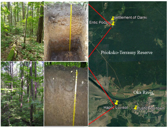
Figure 1.
Study sites, soil profiles (Entic Podzol and Haplic Luvisol) and site locations on the opposite banks of Oka River; Prioksko-Terrasny Reserve is north from the River (“Prioksko-Terrasny Reserve”, 54°52′ N, 37°35′ E, Google Earth. November 2021. 25 May 2023); top left—Entic Podzol and bottom left—Haplic Luvisol soil profiles.
Both forest sites are located in the same moderately-continental climate zone with warm summers and moderately cold winters. Long-term meteorological observations (the Complex Background Monitoring Station, settlement of Danki, Serpukhov district, Moscow region; 54°50′ N, 37°35′ E) for the last 10 years (https://pt-zapovednik.org, accessed on 1 June 2023) report the following: the average annual air temperature is 4.8 °C, the average summer temperature is +17.6 °C (max 38–39 °C), and the average winter temperature is −8.3 °C (min −43 °C in 1978); the average precipitation is 671 mm (max 91 mm in July); the duration of the seasonal snow cover period is 133 days with the average snow depth being 52 cm; the vegetation season lasts 186 days.
Due to the specifics of geomorphology, the soil properties of these sites are quite different (left, Figure 1; Table 1). The higher concentration of fine particles (silt and clay) in the Haplic Luvisol and consequently, smaller pores, explain its higher water-holding capacity and as the result is the lower permittivity to the atmospheric oxygen, reducing SOC oxidation [36], which is directly associated with its higher carbon storage. This process is well investigated on the examples of the wet-meadow and bog soil, having high SOC storage as well [26,37,43,51].

Table 1.
Site description and soil properties of the forest ecosystems.
For the current research, we use a 25-year-long SR-measurement time series conducted by the chambers of the closed type (SR—top, Figure 2) once a week. The standard chamber-measurement approach is described in [20]. Firstly, the repetitive with 10-min interval gas measurements using syringe-sample collection are conducted at sites at five nearby locations to account for SR heterogeneity. Secondly, these samples are analyzed for CO2 concentrations in the laboratory using a gas chromatograph (KrystaLLyuks-4000 M, Meta-Chrom, Yoshkar-Ola, Russia). The obtained changes in CO2 concentration are recalculated into the SR fluxes by applying the chamber volumetric correction [19,22]. Simultaneously with the SR, the soil temperature at 5-cm depth and the air temperature at 1-m height were measured at the sites (Tsoil—brown, Tair—red; middle, Figure 2). The monthly averaged data for the air temperature (Tair) and precipitation (Prec) were collected from the Complex Background Monitoring Station, which is situated nearby to the coniferous-deciduous forest site (blue; bottom, Figure 2). All the data were quality checked and averaged on a monthly base to be fitted into the models.
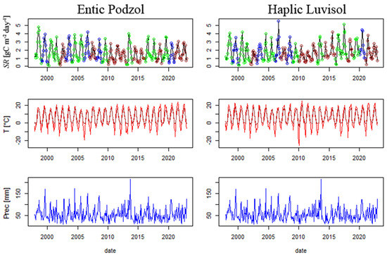
Figure 2.
The 25-year-long measurements of soil respiration (SR, top), temperatures of air and soil (Tair—red and Tsoil—brown, middle), and precipitation (Prec, bottom); on the SR graph: normal conditions—green, wet conditions—blue, dry conditions—brown.
The monthly averaged temperature (T) and precipitation (P) data have also been used for the separation of the years of the measurements into “wet”, “dry”, and “normal” (top, Figure 2) by an application of the following indexes to the data:
- Selyaninov hydrothermal coefficient—, when T > 10 °C (HTC6–8—summer period, June to August months) [53];
- Wetness Indexes— (WI5–8 and WI5–9 for May to August and May to September periods, respectively) [53].
If the values of any of these indexes differ (higher or lower) more than a standard deviation (STD) from the averages for the chosen measurement period, the year was placed into the “wet” or “dry” datasets, respectively. The following 5 years were classified as “wet”—1999, 2003, 2006, 2008, 2020; the following 9 years were “dry”—2002, 2007, 2010, 2011, 2014, 2015, 2018, 2021, 2022; and the remaining 11 years stayed as “normal”—1998, 2000, 2001, 2004, 2005, 2009, 2012, 2013, 2016, 2017, 2019.
For the initialization of the empirical models dependent on SOC, the estimations of the SOC storage in 20-cm layers of Entic Podzol and Haplic Luvisol were used (Table 1).
2.2. Empirical Soil Respiration Models
The current research of the SR estimations is focused on two groups of empirical models connecting SR with the temperature and amount of precipitation, serving as a proxy for the soil moisture [20,24,39,40,41,54] and by this, estimating SR affected by the climatic conditions. The first group includes the models dependent on Tsoil [26,31,32,33], and the second group are the models dependent on Tair [20,24,25,42]. The comparison between the groups shows that both groups are generally based on the same formulations but with using different sources of temperature: Tsoil or Tair.
Temperature and Temperature—Precipitation models [20,24,26,31,32,33]:
Temperature—Precipitation model dependent on the amounts of precipitation for the current (P) and previous (Pm−1) months [25,42]:
Temperature—Precipitation—SOC model [48]:
As an extension from the previous models (Equations (3a) and (4)), we suggest to look at the combined Temperature—Precipitation—SOC model dependent on the amounts of precipitation of two months:
In all models, is the average monthly temperature of the soil surface layer [26,31,32,33] or the average monthly temperature of air [20,24,25,42]; is the average monthly amount of precipitation; is the organic-carbon storage in the top 20-cm of the soil.
The (g C/m2day) is SR at 0 °C in normal soil-humidity conditions—it is usually estimated from the measurements as an average SR for the not-frozen top-soil level. After is identified, the non-linear regression is used to estimate other parameters of the models: and are the exponential-relationship temperature coefficients; (cm) is the half-saturation constant of the hyperbolic relationship between SR and the amount of precipitation; is the redistribution coefficient between the amounts of precipitation for the current (P) and previous (Pm−1) months; and (kg C/m2) is the half-saturation constant of the hyperbolic relationship between SR and SOC.
Practically all the empirical models described above, T (Equation (1))–TP (Equation (2))–TPP (Equation (3a))–TPC (Equation (4))–TPPC (Equation (5)), use the linear temperature dependency in the exponential term and because of it, can be put into the same class of the temperature relationship with SR. On the other hand, the model TPPrh (Equation (3b)) uses the quadratic temperature dependency in the exponential term, which obtains good results when the model was parameterized with the air temperature [25,42], and it was taken to compare with other models.
The quality control of modeling was based on the comparison of the following statistics: the mean bias error (MBE), the root mean square error (RMSE), the slope and intercept of the linear regression (lm) between the measured and modeled data, and the lm determination coefficient (R2).
3. Results and Discussion
3.1. Choice of the
One of the key parameters of all the empirical models described above is —the soil respiration at 0 °C. It significantly affects the modeling quality because it defines the low boundary of the modeling data (winter periods) and the intercept with the ordinate axis of the linear model (lm), comparing modeling and measured data. In the ideal model, the intercept of lm should lay in the origin of the coordinate system and the slope of lm should be equal to 1. However, as a rule for the real models, the slope < 1 and intercept > 0 due to an insufficient magnitude of the modeled data in comparison with the measurements—the extreme values are not represented well by the modeling [20,31,42].
In our research, was estimated from modeling by the T–TP–TPP–TPC–TPPC models in the following way: is directly interconnected with the intercept of lm and by controlling and lowing , the intercept of lm is being readjusted to become positive and closer to zero and at the same time, the slope of lm increases and becomes closer to unity. With the negative intercept of lm, there will be an underestimation of the soil respiration in the winter periods.
The obtained values (colored lines, Figure 3) are two–three times smaller than the earlier obtained values by Raich and Potter (1995) [24] and Kurganova et al. (2020) [20] for the Entic Podzol. They can be directly compared with the SR measurements at 0 ≤ Tsoil < 1 °C in the autumn–winter period (colored dots with labels, Figure 3) when there is not any freezing of the top-soil level, and by the selection of the temperature interval, they should be located closer to the lower SR observed at the lower temperatures (Tsoil ≈ 0).
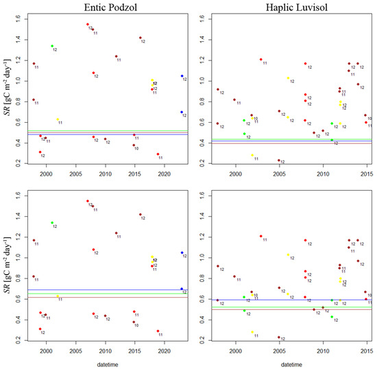
Figure 3.
Parameter —soil respiration in autumn–winter period, Tsoil ≈ 0 °C—values (colored horizontal lines) obtained during modeling by T–TP–TPP–TPC–TPPC models (intercept → 0+) with the parameterization by the soil temperature (top) and the air temperature (bottom, monitoring station) in the normal (green line), wet (blue line), and dry (brown line) years; colored dots with labels—individual SR measurements, where the labels are the measurement-month numbers and the dot colors for the monthly-precipitation amount are red (11 < P < 34 mm), brown (34 < P < 57 mm), yellow (57 < P < 80 mm), green (80 < P < 103 mm), and blue (103 < P < 126 mm).
As the result of such a selection (intercept → 0+), the values obtained for the different set of years—normal (n), wet (w), and dry (d)—demonstrate a weak linear dependency from the soil moisture (colored lines, Figure 3) with the minimal values corresponding mainly with the dry period (brown lines). These maximize the slope of lm (see Table A1, Table A2, Table A3 and Table A4 in the Appendix A) as well.
It should be noted that the values obtained from the models parameterized by Tair are about 15% higher than the values obtained from the models parameterized by Tsoil. This observation can be explained from the differences between Tair and Tsoil for these conditions: the average soil temperature (Tsoil ≈ 2 °C, brown vertical line, Figure 4) is about two degrees higher than the simultaneously observed air temperature (Tair = 0 °C, blue horizontal line, Figure 4), which is associated with the more intensive SR for Tair = 0 °C than for Tsoil = 0 °C.
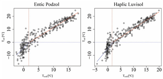
Figure 4.
The interrelationship between Tsoil measured at the sites and Tair obtained from the monitoring station; horizontal blue line—Tair = 0 °C; vertical brown line—average soil temperature Tsoil ≈ 2 °C for Tair ≈ 0 °C; red line—warm-period; and blue line—cold-period linear fits.
The values obtained for different conditions (colored horizontal lines, Figure 3) are close to each other when the parameterization with Tsoil was done. This finding signals that there are more accurate estimations with Tsoil and agrees with Raich and Potter’s (1995) [24] notes on the Q10 temperature coefficients that the microbial biomass responsible for SR is better reacted to the Tsoil changes—the immediate substrate—than to the Tair changes.
This conclusion also agrees well with the observed (Figure 4) significant spread of the air temperatures (Tair ≈ −12–+2 °C) for the soil temperatures close to zero Celsius (Tsoil = 0 °C), seen at both sites and fewer smaller spreads of the soil temperatures (Tsoil ≈ 0–+5 °C) for Tair = 0 °C. On the other hand, the Tsoil ≈ 2 °C threshold serves as a clear indicator of the temperature-regime change. When Tsoil > 2 °C, air and soil temperatures are in a close coupling with each other (red line, Figure 4), while for Tsoil ≤ 2 °C, this coupling behavior has been effectively broken due to the strong influence of liquid water keeping soil from freezing.
The individual values of the measured SR at near zero temperatures, when there is not any freezing of the top-soil level occurred (colored dots, Figure 3), are generally associated with the end-of-the-year cold periods with not very large monthly precipitation (Figure 2). Investigating the large scattering of these SR values, we found some evidence that they depend both on the monthly precipitation and soil properties together. For the Entic Podzol (sandy soil with poor water-holding ability and larger pores), the lower precipitation periods (red and brown dots, Figure 3 left) have the extremely low SR—good drainage easily dries out this soil. However, for Haplic Luvisol (loamy soil with high water-holding ability and smaller pores), the lower precipitation periods (red and brown dots, Figure 3 right) are actually associated with the higher SR—this soil is over saturated with water [36] in cold periods. These evidences point out the importance accounting for the soil properties in SR modeling.
All those mentioned above ensure us that the values we obtained from the modeling (colored horizontal lines, Figure 3) behave as expected in comparison to the measurements.
3.2. Modeling Results
The modeling with the T (Equation (1))–TP (Equation (2))–TPP (Equation (3a))–TPC (Equation (4))–TPPC (Equation (5)) models was conducted with using the non-linear regression for model fitting on the monthly-averaged measured SR, Tsoil or Tair, and precipitation datasets where the winter and summer values were double weighted to obtain the representativeness of the models regardless of the time of the year. In addition to this modeling, the results of the TPPrh (Equation (3b)) modeling with the quadratic temperature dependency were used for comparisons. The temperature-related coefficients и Q were estimated from the T model with using the intercept → 0+ constraint for the lm, comparing the measurements with the modeled data (T, TP, TPP, TPC, TPPC). These coefficient values were taken as the base for further modeling with more complex TP, TPP, TPC, TPPC, and also TPPrh (, Q, and Q2) models. This way, we separate the temperature-related effects (, Q, and Q2) and, sequentially, focus on the precipitation (K) and SOC () effects, and also on the effect of the precipitation redistribution between months (α).
Figure 5 and Figure 6 show that the smallest SR values are observed during the dry years, while the maximal 30% larger values are reached in the normal years, and the SR becomes smaller again during the wet years. These observations agree well with the obtained dependency from the soil moisture (colored lines, Figure 3) and also with the previous research results [55,56,57]. They can be explained by the reduced microbial activity when there is not enough water presented in soil in dry years [32,58,59] and also by the lack of available oxygen for the SOC oxidation when it is saturated with water in wet years [26,36,37].
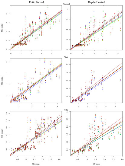
Figure 5.
The comparison between the modeled (SR_model) and measured (SR_meas) SR values (gCm−2day−1) for T (blue, Equation (1)) –TP (green, Equation (2))–TPP (orange, Equation (3a))–TPC (red, Equation (4))–TPPC (black, Equation (5))–TPPrh (brown, Equation (3b)) models; lines—linear regression to determine the slope and intercept values; Tsoil (local temperature) used for parameterizations.
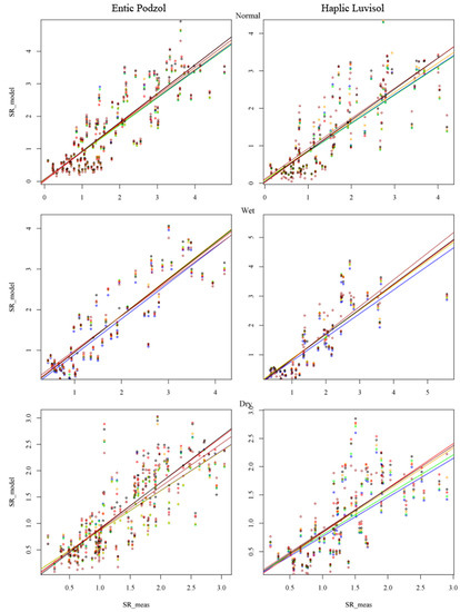
Figure 6.
The comparison between the modeled (SR_model) and measured (SR_meas) SR values (gCm−2day−1) for T (blue, Equation (1)) –TP (green, Equation (2))–TPP (orange, Equation (3a))–TPC (red, Equation (4))–TPPC (black, Equation (5))–TPPrh (brown, Equation (3b)) models; lines—linear regression to determine the slope and intercept values; Tair (monitoring station) used for parameterization.
After fixing the temperature coefficients (R0 и Q) determined by the T–TP–TPP–TPC–TPPC modeling by the method described above (Figure 5 and Figure 6), the comparison among the modeling results shows the following similarities and differences among the models depending on (i) the soil type: Entic Podzol or Haplic Luvisol, and (ii) the sources of the temperature used for parameterization: Tsoil or Tair.
- For Entic Podzol and Tsoil:
- The best slope-lm values (slope, Figure 7) were observed with the TPPC model in a dry environment (slope ≈ 0.9), with the TPC model in a normal environment (slope ≈ 0.9), and with the TPP model in a wet environment (slope ≈ 0.9); the TPPC and TPPrh models show the slope > 0.85 for most of the conditions;
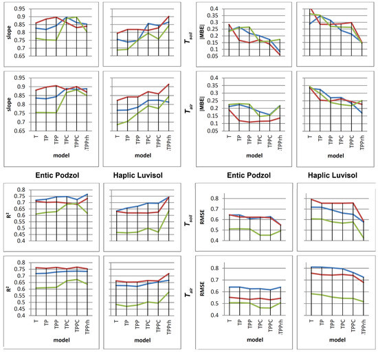 Figure 7. The comparison-statistics: slope—the slope of the lm; R2—the determination coefficient of the lm; —the absolute mean-bias error; and RMSE—the root-mean-square error between the modeled and measures soil Respiration values for the normal (blue), wet (red), and dry (green) environmental conditions; in each panel: top—Tsoil (local), bottom—Tair (monitoring station) used for parameterizations; in each panel: left—for Entic Podzol, right—for Haplic Luvisol.
 - The best R2-lm values (R2, Figure 7) were observed with the TPPC model in a dry environment (R2 ≈ 0.7) and with the TPPrh model in normal and wet environments (R2 ≈ 0.75); the TPPC and TPP models show the R2 > 0.7 for all moisture conditions;
- The best MBE values of the comparison between the models and measurements (, Figure 7) were observed with the TPC and TPPC models in a dry environment ( ≈ 0.15), and with the TPPrh model in normal and wet environments ( ≈ 0.08); the TPPC model shows < 0.17 for all moisture conditions.
- The best RMSE values of the comparison between the models and measurements (RMSE, Figure 7) were observed with the TPC и TPPC in a dry environment (RMSE ≈ 0.45), and with the TPPrh model in normal and wet environments (RMSE ≈ 0.55); the TPPC model shows RMSE < 0.63 for all moisture conditions.
- For Entic Podzol and Tair:
- The best slope lm values (slope, Figure 7) were observed with the TPPC model in dry and wet environments (slope ≈ 0.88–0.9), and with the TPPrh model in a normal environment (slope ≈ 0.88);
- The best R2-lm values (R2, Figure 7) were observed with the TPPC model for all moisture conditions: R2 ≈ 0.67 for dry, R2 ≈ 0.77 for wet, and R2 ≈ 0.74 for normal;
- The best MBE values (, Figure 7) were observed with the TPPC model in normal and dry environments ( ≈ 0.15), while the TPP model gives the smallest ≈ 0.11 in a wet environment;
- The best RMSE values (RMSE, Figure 7) were observed with the TPPC model for all moisture conditions: RMSE ≈ 0.47 for dry, RMSE ≈ 0.53 for wet, and RMSE ≈ 0.63 for normal.
- For Haplic Luvisol and Tsoil:
- The best slope-lm values (slope, Figure 7) were observed with the TPPrh for all moisture conditions (slope ≈ 0.85–0.9);
- The best R2-lm values (R2, Figure 7) were observed with the TPPrh for all moisture conditions (R2 ≈ 0.65–0.75);
- The best MBE values (, Figure 7) were observed with the TPPrh for all moisture conditions ( ≈ 0.15);
- The best RMSE values (RMSE, Figure 7) were observed with the TPPrh for all moisture conditions (RMSE ≈ 0.43–0.53).
- For Haplic Luvisol and Tair:
- The best slope-lm values (slope, Figure 7) were observed with the TPPrh model in dry and wet environments (slope ≈ 0.85–0.91), and with the TPC and TPPC models in a normal environment (slope ≈ 0.85);
- The best R2-lm values (R2, Figure 7) were observed with the TPPrh for all moisture conditions (R2 ≈ 0.57–0.73);
- The best MBE values (, Figure 7) were observed with the TPPrh model in normal and wet environments ( ≈ 0.15–0.23), and with the TPPC model in a dry environment ( ≈ 0.23);
- The best RMSE values (RMSE, Figure 7) were observed with the TPPrh for all moisture conditions (RMSE ≈ 0.53–0.73).
From the conducted analysis, we see that the SOC and water-holding abilities are critical for the choice of optimal SR models. The TPPrh model with the quadratic dependency on the temperature becomes more optimal in most of the environmental conditions—normal, dry, and wet—for Haplic Luvisol having the finer texture (siltic), meaning lower permittivity to gasses [36], and the ability to hold larger amounts of water in comparison to Entic Podzol (Table 1) and for a longer time period. On the other hand, the TPPC model looks more optimal for sandy Entic Podzol, for which the weak water-holding ability leads to lack of water in the dry periods and brings forward the presence of SOC—as the substrate for the microbial community—to support SR when precipitation occurs.
These conclusions are also supported by the comparison of the mean annual SR measurements with modeled values (Figure 8). While the TPPrh model shows a better annual performance for Tsoil, for Tair, the TPPC model becomes slightly better for Entic Podzol—the respective SR measured and modeled values stay within the standard deviation ranges of each other. However, it should be noted that these conclusions based on the annual means can be biased toward the larger summer SR values, underestimating the effects of the smaller winter SR. The underestimation of the mean annual SR is also in agreement with the fact that the model-comparison slopes are smaller than unity for both Entic Podzol (Figure 5) and Haplic Luvisol (Figure 6), causing a possible underestimation of the larger summer-time SR values. In the next section, we will see that the lower winter-time SR values are actually adequately modeled by our procedure and should not influence the respective model behavior showed in Figure 8.
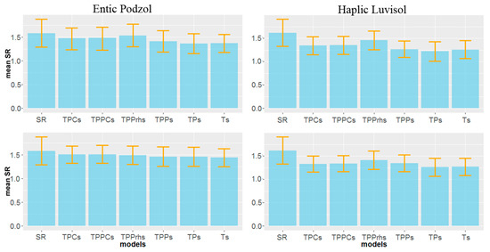
Figure 8.
The mean annual SR (gC m−2 day−1) over 25-year-long periods—blue bars—measured (SR) and modeled (labels on the x-axis) with the standard deviation ranges (orange bars) of the individual-year distributions of the mean annual SR; top—Tsoil (local), bottom—Tair (monitoring station).
3.3. An Optimal-Model Selection and the Winter Soil Respiration Control
The obtained above conclusions on the quality of the SR models parameterized with the different temperature sources (Tsoil and Tair) for Entic Podzol (Figure 9) and Haplic Luvisol (Figure 10) are well illustrated by the time series generated from the TPPC (red) and TPPrh (blue) models. It should be noted that the TPPC model generates higher values than the TPPrh model and by this, the TPPC model better approximates the winter extremes but overestimates the summer SR pikes. It can be seen that an application of Tsoil for the model parameterization allows more accurate estimations of the winter SR (both models) and reduces overestimations in summer (both models), improving SR estimates in the warm periods.
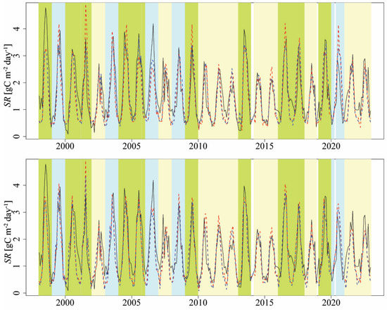
Figure 9.
The SR time series modeling for Entic Podzol: SR measurements—black line, TPPC model—dashed red line, and TPPrh model—dashed blue line; top—for Tsoil (local) and bottom—for Tair (monitoring station); green—normal, blue—wet, beige—dry years.
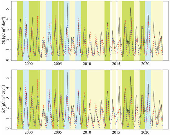
Figure 10.
The SR time series modeling for Haplic Luvisol: SR measurements—black line, TPPC model—dashed red line, and TPPrh model—dashed blue line; top—for Tsoil (local) and bottom—for Tair (monitoring station); green—normal, blue—wet, beige—dry years.
As an explanation of such model behavior, we can point to the soil condition difference between the winter and summer periods: when there is enough water in winters, the SR becomes more dependent on the Tsoil interconnected with microbial activity and SOC presence as a substrate for the microbial community [24], while in dryer summer periods, the presence of precipitation and the respective temperature and humidity changes though the evapotranspiration of vegetation [60,61] start playing an important role in the soil water balance and SR regulation. All those mentioned above are illustrated by Figure 4 (Section 3.1) highlighting different regimes of dependency between the Tsoil and Tair in the cold and warm times of the year—blue and red lines, respectively.
We combine the TPPC and TPPrh models by the regime-change condition (Tsoil ≈ 2 °C) from Figure 4, comparing the soil and air temperatures:
- with the Tsoil > 2 °C—choose the TPPrh model;
- with the Tsoil ≤ 2 °C—choose the TPPC model.
For the comparison analysis of the combined TPPC, the TPPrh models (Table 2) show the best statistical values for R2, MBE, and RMSE for the following model parameterizations:
All data: for the combined TPPC[Tsoil], the TPPrh[Tsoil] model parameterized by the soil temperature;
Cold period: for the TPPC[Tsoil] model parameterized by the soil temperature;
Warm period: for the TPPrh[Tsoil] or TPPrh[Tair] model parameterized by the soil or the air temperature.
Table 2.
Quality control of the modeling by the combined TPPC: TPPrh models with the parameterization by different temperature sources ([Tsoil] or [Tair]) conducted on the 25-year monitoring for Entic Podzol and Haplic Luvisol; top—all data, middle—cold periods (Tsoil ≤ 2 °C), bottom—warm periods (Tsoil > 2 °C).
| Entic Podzol | Haplic Luvisol | |||||
|---|---|---|---|---|---|---|
| Model | R2 | MBE | RMSE | R2 | MBE | RMSE |
| (all data) | ||||||
| TPPC[Tsoil]:TPPrh[Tair] | 0.734 | −0.150 | 0.527 | 0.624 | −0.348 | 0.716 |
| TPPC[Tair]:TPPrh[Tair] | 0.731 | −0.156 | 0.536 | 0.623 | −0.357 | 0.723 |
| TPPC[Tsoil]:TPPrh[Tsoil] | 0.735 | −0.115 | 0.524 | 0.674 | −0.287 | 0.651 |
| Tsoil ≤ 2 (cold periods) | ||||||
| TPPC[Tsoil] | 0.116 | −0.225 | 0.397 | 0.054 | −0.376 | 0.553 |
| TPPC[Tair] | 0.110 | −0.241 | 0.428 | 0.047 | −0.402 | 0.580 |
| TPPrh[Tsoil] | 0.032 | −0.224 | 0.411 | 0.110 | −0.425 | 0.581 |
| TPPrh[Tair] | 0.070 | −0.288 | 0.480 | 0.040 | −0.456 | 0.643 |
| Tsoil > 2 (warm periods) | ||||||
| TPPC[Tsoil] | 0.583 | −0.124 | 0.638 | 0.465 | −0.413 | 0.852 |
| TPPC[Tair] | 0.616 | −0.094 | 0.599 | 0.431 | −0.412 | 0.856 |
| TPPrh[Tsoil] | 0.604 | −0.051 | 0.584 | 0.512 | −0.239 | 0.698 |
| TPPrh[Tair] | 0.604 | −0.106 | 0.589 | 0.431 | −0.333 | 0.790 |
It should be noted that the (intercept → 0+) approach which we developed guarantees an adequate estimation of the cold-period SR and a good magnitude resolution of the model results (confirmed by Figure 8) in comparison to the measurements—an often observed inefficiency of the standard parameterization approaches [20,31,42].
For Haplic Luvisol (Figure 10), the SR measurements are well represented by the modeling values before the 2015 year; however, in the later period, the winter-time SR values are too large due to changes in the forest structure (tree fall down) that year, making soil more accessible to elements [62].
The low R2 values for the cold period (Table 2) are directly associated with the high variability of the observations (see Figure 3) which typically occur during the winter-time measurements due to snow presence on the ground and freezing–thawing cycles and also due to changes in precipitation causing CO2 accumulation in soil and interrupting gas exchange.
4. Conclusions
We have demonstrated an importance to account for the SOC storage and water-holding ability for the selection of the proper SR models. For the sandy Entic Podzol with a coarse texture and good drainage, it is better to use the models accounting for the SOC storage (TPC and TPPC), while for the loamy Haplic Luvisol, having a finer texture and high water-holding ability, it is better to apply Raich–Hashimoto-type models (TPPrh) with the quadratic temperature dependency being connected to the water presence in the soil and the reaction of the microbial biomass on temperature change.
Both in the dry and in the normal years, accounting for SOC storage significantly improves the modeling results (TPC and TPPC models) in comparison to the more simple model results (T, TP, and TPP models). In the dry years, the TPPC model is better than the TPC model, but in the normal years, the TPC model is better than the TPPC model, highlighting an importance of the prolonged presence of soil humidity in dry periods.
An effect of humidity change becomes the most important in the wet years (TPP и TPPC models). Optimal values for the parameter included into the TPP and TPPC models become close to zero or negative in the dry years, highlighting an importance of the (continuous) moisture and precipitation presence from the previous month (PP).
We found that TPPC parameterized by the soil temperature adequately describes the SR measured during the cold periods (Tsoil ≤ 2 °C), whereas TPPrh parameterized by the soil or air temperature is better for describing the SR measured during the warm periods (Tsoil > 2 °C).
The parameterization of the models with the soil temperature is shown to be an important factor for adequate SR estimates. With this parameterization, the TPPC model can be applied for the control of the winter-time SR measurements conducted at the sites.
Author Contributions
Conceptualization, I.K. and S.K.; methodology, I.K. and S.K.; formal analysis, S.K.; investigation, S.K.; resources, V.L.d.G., D.K., T.M. and D.S.; data curation, V.L.d.G., D.K. and S.K.; writing—original draft preparation, S.K.; writing—review and editing, I.K., K.I. and S.K.; visualization, D.K., V.L.d.G. and S.K.; supervision, I.K. and K.I.; project administration, I.K. and K.I.; funding acquisition, I.K. and K.I. All authors have read and agreed to the published version of the manuscript.
Funding
The data collection and preparation were carried out as part of the most important innovative project of national importance, “Development of a system for ground-based and remote monitoring of carbon pools and greenhouse gas fluxes in the territory of the Russian Federation, ensuring the creation of recording data systems on the fluxes of climate-active substances and the carbon budget in forests and other terrestrial ecological systems” (Registration number: 123030300031-6); the data analysis and modeling works were supported by state assignment No. 122111000095-8.
Data Availability Statement
The data presented in this study are available on reasonable request from the authors.
Acknowledgments
We give thanks to Vera Ableeva (Station of Background Monitoring, Roshydromet) who provides us the meteorological data set (1973 to 2021) for the study area. We especially thank Daniela Dalmonech for her comments and suggestions improving the objectivity of the better model selection process and anonymous reviewers for their constructive comments.
Conflicts of Interest
The authors declare no conflict of interest.
Appendix A
The results of parameterizations of the models and the comparisons between the soil Respiration measurements and modeling results for the Entic Podzol (Table A1 and Table A3) and Haplic Luvisol (Table A2 and Table A4); Tsoil or Tair was used for the model parameterizations.
Table A1.
Parameters (, Q, Q2, K, , ) of the models (T, TP, TPP, TPC, TPPC, TPPrh) and the comparisons with the measurements (|MBE|, RMSE, slope, intercept, R2) for the Entic Podzol and forest ecosystem in normal (n), wet (w), and dry (d) years; Tsoil was used for the model parameterizations.
Table A1.
Parameters (, Q, Q2, K, , ) of the models (T, TP, TPP, TPC, TPPC, TPPrh) and the comparisons with the measurements (|MBE|, RMSE, slope, intercept, R2) for the Entic Podzol and forest ecosystem in normal (n), wet (w), and dry (d) years; Tsoil was used for the model parameterizations.
| Model | Wetness | Q | Q2 | K | Slope | Intercept | |MBE| | RMSE | R2 | |||
|---|---|---|---|---|---|---|---|---|---|---|---|---|
| T | n | 0.545 | 0.118 | - | - | - | - | 0.827 | 0.063 | 0.237 | 0.643 | 0.720 |
| TP | n | 0.545 | 0.118 | - | 0.901 | - | - | 0.819 | 0.049 | 0.266 | 0.644 | 0.726 |
| TPP | n | 0.545 | 0.118 | - | −0.941 | 1.137 | - | 0.843 | 0.054 | 0.219 | 0.609 | 0.745 |
| TPC | n | 0.545 | 0.118 | - | 6.838 | - | −0.179 | 0.897 | −0.022 | 0.200 | 0.617 | 0.747 |
| TPPC | n | 0.545 | 0.118 | - | −0.571 | 1.753 | −0.043 | 0.863 | 0.066 | 0.172 | 0.628 | 0.724 |
| TPPrh | n | 0.545 | 0.197 | 0.005 | −1.694 | 2.266 | - | 0.853 | 0.172 | 0.083 | 0.549 | 0.765 |
| T | w | 0.508 | 0.121 | - | - | - | - | 0.860 | −0.044 | 0.284 | 0.645 | 0.711 |
| TP | w | 0.508 | 0.121 | - | −4.341 | - | - | 0.885 | 0.029 | 0.167 | 0.625 | 0.702 |
| TPP | w | 0.508 | 0.121 | - | −4.954 | 0.072 | - | 0.897 | 0.026 | 0.149 | 0.623 | 0.704 |
| TPC | w | 0.508 | 0.121 | - | −5.869 | - | 0.042 | 0.863 | 0.063 | 0.171 | 0.623 | 0.697 |
| TPPC | w | 0.508 | 0.121 | - | −11.137 | 0.330 | 0.148 | 0.831 | 0.152 | 0.138 | 0.617 | 0.686 |
| TPPrh | w | 0.508 | 0.188 | 0.005 | −5.843 | 0.119 | - | 0.840 | 0.214 | 0.060 | 0.548 | 0.732 |
| T | d | 0.526 | 0.094 | - | - | - | - | 0.763 | 0.095 | 0.233 | 0.511 | 0.610 |
| TP | d | 0.526 | 0.094 | - | 0.864 | - | - | 0.753 | 0.082 | 0.261 | 0.512 | 0.623 |
| TPP | d | 0.526 | 0.094 | - | 0.734 | 1.157 | - | 0.751 | 0.081 | 0.265 | 0.510 | 0.629 |
| TPC | d | 0.526 | 0.094 | - | 12.374 | - | −0.353 | 0.889 | −0.003 | 0.157 | 0.451 | 0.688 |
| TPPC | d | 0.526 | 0.094 | - | 20.012 | 0.870 | −0.440 | 0.898 | −0.019 | 0.161 | 0.452 | 0.692 |
| TPPrh | d | 0.526 | 0.094 | 0.005 | 0.734 | 1.157 | - | 0.805 | 0.097 | 0.174 | 0.493 | 0.617 |
Table A2.
Parameters (, Q, Q2, K, , ) of the models (T, TP, TPP, TPC, TPPC, TPPrh) and the comparisons with the measurements (|MBE|, RMSE, slope, intercept, R2) for the Haplic Luvisol and forest ecosystem in normal (n), wet (w), and dry (d) years; Tsoil was used for the model parameterizations.
Table A2.
Parameters (, Q, Q2, K, , ) of the models (T, TP, TPP, TPC, TPPC, TPPrh) and the comparisons with the measurements (|MBE|, RMSE, slope, intercept, R2) for the Haplic Luvisol and forest ecosystem in normal (n), wet (w), and dry (d) years; Tsoil was used for the model parameterizations.
| Model | Wetness | Q | Q2 | K | Slope | Intercept | |MBE| | RMSE | R2 | |||
|---|---|---|---|---|---|---|---|---|---|---|---|---|
| T | n | 0.448 | 0.119 | - | - | - | - | 0.755 | 0.112 | 0.287 | 0.718 | 0.635 |
| TP | n | 0.448 | 0.119 | - | 2.179 | - | - | 0.738 | 0.079 | 0.347 | 0.717 | 0.658 |
| TPP | n | 0.448 | 0.119 | - | 0.181 | 1.129 | - | 0.747 | 0.097 | 0.315 | 0.690 | 0.671 |
| TPC | n | 0.448 | 0.119 | - | 10.960 | - | −1.050 | 0.856 | −0.006 | 0.239 | 0.662 | 0.696 |
| TPPC | n | 0.448 | 0.119 | - | 4.537 | 1.099 | −0.767 | 0.843 | 0.044 | 0.212 | 0.650 | 0.694 |
| TPPrh | n | 0.448 | 0.238 | 0.007 | 7.495 | 1.036 | - | 0.865 | 0.070 | 0.150 | 0.577 | 0.742 |
| T | w | 0.432 | 0.122 | - | - | - | - | 0.794 | −0.055 | 0.416 | 0.792 | 0.631 |
| TP | w | 0.432 | 0.122 | - | −5.128 | - | - | 0.818 | 0.035 | 0.285 | 0.756 | 0.619 |
| TPP | w | 0.432 | 0.122 | - | −5.151 | 0.995 | - | 0.818 | 0.035 | 0.285 | 0.756 | 0.619 |
| TPC | w | 0.432 | 0.122 | - | −5.316 | - | 0.030 | 0.813 | 0.039 | 0.288 | 0.756 | 0.618 |
| TPPC | w | 0.432 | 0.122 | - | −2.683 | 1.298 | −0.124 | 0.828 | 0.004 | 0.298 | 0.757 | 0.626 |
| TPPrh | w | 0.432 | 0.239 | 0.007 | −0.030 | 1.537 | - | 0.902 | 0.022 | 0.150 | 0.587 | 0.742 |
| T | d | 0.408 | 0.093 | - | - | - | - | 0.687 | 0.057 | 0.363 | 0.607 | 0.467 |
| TP | d | 0.408 | 0.093 | - | −0.356 | - | - | 0.691 | 0.061 | 0.352 | 0.605 | 0.463 |
| TPP | d | 0.408 | 0.093 | - | −2.952 | 0.037 | - | 0.751 | 0.064 | 0.269 | 0.578 | 0.469 |
| TPC | d | 0.408 | 0.093 | - | 6.617 | - | −1.147 | 0.794 | 0.012 | 0.264 | 0.567 | 0.500 |
| TPPC | d | 0.408 | 0.093 | - | −1.954 | 0.009 | −0.180 | 0.757 | 0.064 | 0.262 | 0.577 | 0.469 |
| TPPrh | d | 0.408 | 0.221 | 0.008 | −3.074 | 0.384 | - | 0.842 | 0.069 | 0.143 | 0.426 | 0.635 |
Table A3.
Parameters (, Q, Q2, K, , ) of the models (T, TP, TPP, TPC, TPPC, TPPrh) and the comparisons with the measurements (|MBE|, RMSE, slope, intercept, R2) for the Entic Podzol and forest ecosystem in normal (n), wet (w), and dry (d) years; Tair (meteostation) was used for parameterization.
Table A3.
Parameters (, Q, Q2, K, , ) of the models (T, TP, TPP, TPC, TPPC, TPPrh) and the comparisons with the measurements (|MBE|, RMSE, slope, intercept, R2) for the Entic Podzol and forest ecosystem in normal (n), wet (w), and dry (d) years; Tair (meteostation) was used for parameterization.
| Model | Wetness | Q | Q2 | K | Slope | Intercept | |MBE| | RMSE | R2 | |||
|---|---|---|---|---|---|---|---|---|---|---|---|---|
| T | n | 0.686 | 0.087 | - | - | - | - | 0.836 | 0.074 | 0.211 | 0.640 | 0.717 |
| TP | n | 0.686 | 0.087 | - | 0.384 | - | - | 0.832 | 0.067 | 0.224 | 0.640 | 0.720 |
| TPP | n | 0.686 | 0.087 | - | −0.473 | 1.135 | - | 0.844 | 0.066 | 0.205 | 0.625 | 0.729 |
| TPC | n | 0.686 | 0.087 | - | 4.362 | - | −0.128 | 0.890 | 0.013 | 0.177 | 0.626 | 0.734 |
| TPPC | n | 0.686 | 0.087 | - | 1.001 | 1.122 | −0.079 | 0.885 | 0.042 | 0.157 | 0.616 | 0.736 |
| TPPrh | n | 0.618 | 0.121 | 0.002 | 0.273 | 1.128 | - | 0.889 | −0.025 | 0.218 | 0.639 | 0.734 |
| T | w | 0.724 | 0.082 | - | - | - | - | 0.881 | 0.014 | 0.191 | 0.553 | 0.762 |
| TP | w | 0.724 | 0.082 | - | −2.618 | - | - | 0.898 | 0.056 | 0.118 | 0.544 | 0.757 |
| TPP | w | 0.724 | 0.082 | - | −2.171 | 1.331 | - | 0.906 | 0.052 | 0.109 | 0.536 | 0.764 |
| TPC | w | 0.724 | 0.082 | - | −4.089 | - | 0.032 | 0.884 | 0.083 | 0.114 | 0.544 | 0.753 |
| TPPC | w | 0.724 | 0.082 | - | −1.114 | −2.042 | −0.055 | 0.901 | 0.054 | 0.116 | 0.532 | 0.766 |
| TPPrh | w | 0.651 | 0.095 | 0.001 | −4.949 | 1.249 | - | 0.870 | 0.087 | 0.136 | 0.544 | 0.753 |
| T | d | 0.649 | 0.063 | - | - | - | - | 0.755 | 0.114 | 0.225 | 0.507 | 0.608 |
| TP | d | 0.649 | 0.063 | - | 0.167 | - | - | 0.754 | 0.111 | 0.231 | 0.507 | 0.611 |
| TPP | d | 0.649 | 0.063 | - | −0.750 | 2.586 | - | 0.753 | 0.116 | 0.227 | 0.503 | 0.613 |
| TPC | d | 0.649 | 0.063 | - | 8.757 | - | −0.291 | 0.867 | 0.038 | 0.147 | 0.464 | 0.662 |
| TPPC | d | 0.649 | 0.063 | - | 20.364 | 0.763 | −0.435 | 0.883 | 0.009 | 0.153 | 0.462 | 0.672 |
| TPPrh | d | 0.584 | 0.110 | 0.002 | 0.084 | 1.234 | - | 0.850 | −0.008 | 0.216 | 0.506 | 0.637 |
Table A4.
Parameters (, Q, Q2, K, , ) of the models (T, TP, TPP, TPC, TPPC, TPPrh) and the comparisons with the measurements (|MBE|, RMSE, slope, intercept, R2) for the Haplic Luvisol and forest ecosystem in normal (n), wet (w), and dry (d) years; Tair (meteostation) was used for parameterization.
Table A4.
Parameters (, Q, Q2, K, , ) of the models (T, TP, TPP, TPC, TPPC, TPPrh) and the comparisons with the measurements (|MBE|, RMSE, slope, intercept, R2) for the Haplic Luvisol and forest ecosystem in normal (n), wet (w), and dry (d) years; Tair (meteostation) was used for parameterization.
| Model | Wetness | Q | Q2 | K | Slope | Intercept | |MBE| | RMSE | R2 | |||
|---|---|---|---|---|---|---|---|---|---|---|---|---|
| T | n | 0.538 | 0.100 | - | - | - | - | 0.767 | 0.103 | 0.331 | 0.810 | 0.628 |
| TP | n | 0.538 | 0.100 | - | −0.204 | - | - | 0.768 | 0.107 | 0.325 | 0.809 | 0.627 |
| TPP | n | 0.538 | 0.100 | - | −2.136 | 0.440 | - | 0.784 | 0.133 | 0.270 | 0.803 | 0.621 |
| TPC | n | 0.538 | 0.100 | - | 3.588 | - | −0.522 | 0.823 | 0.058 | 0.272 | 0.795 | 0.640 |
| TPPC | n | 0.538 | 0.100 | - | −0.946 | −0.933 | −0.202 | 0.824 | 0.094 | 0.233 | 0.764 | 0.654 |
| TPPrh | n | 0.538 | 0.175 | 0.004 | −0.346 | 2.364 | - | 0.813 | 0.178 | 0.170 | 0.724 | 0.667 |
| T | w | 0.611 | 0.093 | - | - | - | - | 0.823 | −0.007 | 0.338 | 0.758 | 0.662 |
| TP | w | 0.611 | 0.093 | - | −3.108 | - | - | 0.842 | 0.041 | 0.254 | 0.745 | 0.654 |
| TPP | w | 0.611 | 0.093 | - | −2.787 | 1.268 | - | 0.842 | 0.046 | 0.249 | 0.742 | 0.655 |
| TPC | w | 0.611 | 0.093 | - | 1.107 | - | −0.318 | 0.872 | −0.023 | 0.263 | 0.747 | 0.665 |
| TPPC | w | 0.611 | 0.093 | - | −0.242 | 2.004 | −0.232 | 0.860 | 0.018 | 0.245 | 0.739 | 0.662 |
| TPPrh | w | 0.611 | 0.158 | 0.003 | 3.576 | −0.618 | - | 0.914 | −0.066 | 0.227 | 0.680 | 0.718 |
| T | d | 0.530 | 0.065 | - | - | - | - | 0.686 | 0.078 | 0.343 | 0.584 | 0.485 |
| TP | d | 0.530 | 0.065 | - | −1.484 | - | - | 0.704 | 0.098 | 0.298 | 0.574 | 0.470 |
| TPP | d | 0.530 | 0.065 | - | −3.552 | 0.156 | - | 0.750 | 0.096 | 0.239 | 0.555 | 0.480 |
| TPC | d | 0.530 | 0.065 | - | 3.968 | - | −0.969 | 0.792 | 0.053 | 0.225 | 0.545 | 0.504 |
| TPPC | d | 0.530 | 0.065 | - | −0.013 | −0.432 | −0.595 | 0.777 | 0.081 | 0.218 | 0.543 | 0.495 |
| TPPrh | d | 0.530 | 0.126 | 0.003 | −0.011 | −0.432 | - | 0.844 | −0.043 | 0.251 | 0.516 | 0.578 |
References
- Ryan, M.; Law, B. Interpreting, measuring, and modeling soil respiration. Biogeochemistry 2005, 73, 3–27. [Google Scholar] [CrossRef]
- Le Quéré, C.; Moriarty, R.; Andrew, R.M.; Peters, G.P.; Ciais, P.; Friedlingstein, P.; Jones, S.D.; Sitch, S.; Tans, P.; Arneth, A.; et al. Global carbon budget 2014. Earth Syst. Sci. Data 2015, 7, 47–85. [Google Scholar] [CrossRef]
- Valentini, R.; Matteucci, G.; Dolman, A.J.; Schulze, E.D.; Rebmann, C.; Moors, E.J.; Granier, A.; Gross, P.; Jensen, N.O.; Pilegaard, K.; et al. Respiration as the main determinant of carbon balance in European forests. Nature 2000, 404, 861–865. [Google Scholar] [CrossRef] [PubMed]
- Peltoniemi, M.; Thürig, E.; Ogle, S.; Palosuo, T.; Schrumpf, M.; Wutzler, T.; Butterbach-Bahl, K.; Chertov, O.; Komarov, A.; Mikhailov, A.; et al. Models in country scale carbon accounting of forest soils. Silva Fenn. 2007, 41, 575–602. [Google Scholar] [CrossRef]
- Lovett, G.M.; Cole, J.J.; Pace, M.L. Is Net Ecosystem Production Equal to Ecosystem Carbon Accumulation? Ecosystems 2006, 9, 152–155. [Google Scholar] [CrossRef]
- Chapin, F.S., III; Woodwell, G.M.; Randerson, J.T.; Rastetter, E.B.; Lovett, G.M.; Baldocchi, D.D.; Clark, D.A.; Harmon, M.E.; Schimel, D.S.; Valentini, R.; et al. Reconciling Carbon-Cycle Concepts, Terminology, and Methods. Ecosystems 2006, 9, 1041–1050. [Google Scholar] [CrossRef]
- UNFCCC. National Inventory Submissions. 2006. Available online: http://unfccc.int/national_reports/annex_i_ghg_inventories/national_inventories_submissions/items/3734.php (accessed on 1 June 2023).
- Singh, B.K. (Ed.) Soil Carbon Storage: Modulators, Mechanisms and Modeling; Academic Press: London, UK, 2018. [Google Scholar]
- Kirschbaum, M.U.F.; Eamus, D.; Gifford, R.M.; Roxburgh, G.H.; Sands, P.J. Definitions of Some Ecological Terms Commonly Used in Carbon Accounting. In Net Ecosystem Exchange Workshop Proceedings CRC for Greenhouse Accounting; Kirschbaum, M.U.F., Mueller, R., Eds.; Canberra Act: Canbera, Australia, 2001; pp. 2–5. [Google Scholar]
- Aubinet, M.; Vesala, T.; Papale, D. (Eds.) Eddy Covariance; Springer: Dordrecht, The Netherlands, 2012. [Google Scholar]
- Burba, G. Eddy Covariance Method for Scientific, Industrial, Agricultural, and Regulatory Applications: A Field Book on Measuring Ecosystem Gas Exchange and Areal Emission Rates; LI-COR Biosciences: Lincoln, NE, USA, 2013. [Google Scholar]
- Baldocchi, D.D. Measuring fluxes of trace gases and energy between ecosystems and the atmosphere—The state and future of the eddy covariance method. Glob. Chang. Biol. 2014, 20, 3600–3609. [Google Scholar] [CrossRef]
- Baldocchi, D.D.; Chu, H.; Reichstein, M. Inter-annual variability of net and gross ecosystem carbon fluxes: A review. Agric. For. Meteorol. 2017, 249, 520–533. [Google Scholar] [CrossRef]
- Reichstein, M.; Falge, E.; Baldocchi, D.; Papale, D.; Aubient, M.; Berbiger, P.; Bernhofer, C.; Buchmann, N.; Gilmanov, T.; Garnier, A.; et al. On the separation of net ecosystem exchange into assimilation and ecosystem respiration: Review and improved algorithm. Glob. Chang. Biol. 2005, 11, 1424–1439. [Google Scholar] [CrossRef]
- Kutsch, W.; Bahn, M.; Heinemeyer, A. Soil Carbon Dynamics; Cambridge University Press: Cambridge, UK, 2009. [Google Scholar]
- Vekuri, H.; Tuovinen, J.P.; Kulmala, L.; Papale, D.; Kolari, P.; Aurela, M.; Laurila, T.; Liski, J.; Lohila, A. A widely-used eddy covariance gap-filling method creates systematic bias in carbon balance estimates. Sci. Rep. 2023, 13, 1720. [Google Scholar] [CrossRef]
- Hanson, P.J.; Edwards, N.T.; Garten, C.T.; Andrews, J.A. Separating root and soil microbial contributions to soil respiration: A review of methods and observations. Biogeochemistry 2000, 48, 115–146. [Google Scholar] [CrossRef]
- Lopes De Gerenyu, V.O.; Kurganova, I.N.; Rozanova, L.N.; Kudeyarov, V.N. Annual emission of carbon dioxide from soils of the southern taiga zone of Russia. Eurasian Soil Sci. 2001, 34, 931–944. [Google Scholar]
- Kurganova, I.; Lopes de Gerenyu, V.; Rozanova, L.; Sapronov, D.; Myakshina, T.; Kudeyarov, V. Annual and seasonal CO2 fluxes from Russian southern taiga soils. Tellus B Chem. Phys. Meteorol. 2003, 55, 338–344. [Google Scholar] [CrossRef]
- Kurganova, I.N.; Lopes de Gerenyu, V.O.; Myakshina, T.N.; Sapronov, D.V.; Romashkin, I.V.; Zhmurin, V.A.; Kudeyarov, V.N. Native and model assessment of Respiration of forest sod-podzolic soil in Prioksko-Terrasny Biospheric Reserve. Contemp. Probl. Ecol. 2020, 13, 813–824. [Google Scholar] [CrossRef]
- Kurganova, I.N.; Lopes de Gerenyu, V.O.; Khoroshaev, D.A.; Blagodatskaya, E. Effect of snowpack pattern on cold-season CO2 efflux from soils under temperate continental climate. Geoderma 2017, 304, 28–39. [Google Scholar] [CrossRef]
- Kurganova, I.N.; Lopes de Gerenyu, V.O.; Khoroshaev, D.A.; Myakshina, T.N.; Sapronov, D.V.; Zhmurin, V.A.; Kudeyarov, V.N. Analysis of the Long-Term Soil Respiration Dynamics in the Forest and Meadow Cenoses of the Prioksko-Terrasny Biosphere Reserve in the Perspective of Current Climate Trends. Eurasian Soil Sci. 2020, 53, 1421–1436. [Google Scholar] [CrossRef]
- Reichstein, M.; Rey, A.; Freibauer, A.; Tenhunen, J.; Valnetini, R.; Banza, J.; Caslas, P.; Cheng, Y.; Grunzweig, J.M.; Irvine, J.; et al. Modeling temporal and large-scale spatial variability of soil respiration from soil water availability, temperature and vegetation productivity indices. Glob. Biogeochem. Cycles 2003, 17, 1104. [Google Scholar] [CrossRef]
- Raich, J.W.; Potter, C.S. Global patterns of carbon dioxide emission from soils. Glob. Biogeochem. Cycles 1995, 9, 23–36. [Google Scholar] [CrossRef]
- Hashimoto, S.; Carvalhais, N.; Ito, A.; Migliavacca, M.; Nishina, K.; Reichstein, M. Global spatiotemporal distribution of soil respiration modeled using a global database. Biogeosciences 2015, 12, 4121–4132. [Google Scholar] [CrossRef]
- Pavelka, M.; Darenova, E.; Dusek, J. Modeling of soil CO2 efflux during water table fluctuation based on in situ measured data from a sedge-grass marsh. Appl. Ecol. Environ. Res. 2016, 14, 423–437. [Google Scholar] [CrossRef]
- Komarov, A.S.; Chertov, O.G.; Nadporozhskaya, M.A.; Priputina, I.V. Models of Forest Soil Organic Matter Dynamics; Kudeyarov, V.N., Ed.; Nauka: Moscow, Russia, 2007; 380p. (In Russian) [Google Scholar]
- Chertov, O.G.; Nadporozhskaya, M.A. Models of soil organic matter dynamics: Problems and perspectives. Comput. Res. Model. 2016, 8, 391–399. (In Russian) [Google Scholar] [CrossRef]
- Priputina, I.V.; Bykhovets, S.S.; Frolov, P.V.; Chertov, O.G.; Kurganova, I.N.; Lopes de Gerenyu, V.O.; Sapronov, D.V.; Myakshina, T.N. Application of Mathematical Models ROMUL and Romul_Hum for Estimating CO2 Emissions and Dynamics of Organic Matter in Albic Luvisol under Deciduous Forest in Southern Moscow Region. Eurasian Soil Sci. 2020, 53, 1480–1491. [Google Scholar] [CrossRef]
- Lopes De Gerenyu, V.O.; Kurganova, I.N.; Rozanova, L.N.; Kudeyarov, V.N. Effect of temperature and moisture on CO2 evolution rate of cultivated Phaeozem: Analyses of long-term field experiment. Plant Soil Environ. 2005, 51, 213–219. [Google Scholar] [CrossRef]
- Juhász, C.; Huzsvai, L.; Kovács, E.; Kovács, G.; Tuba, G.; Sinka, L.; Zsembeli, J. Carbon Dioxide Efflux of Bare Soil as a Function of Soil Temperature and Moisture Content under Weather Conditions of Warm, Temperate, Dry Climate Zone. Agronomy 2022, 12, 3050. [Google Scholar] [CrossRef]
- Howard, P.J.A.; Howard, D.M. Respiration of decomposing litter in relation to temperature and moisture. Oikos 1979, 33, 457465. [Google Scholar] [CrossRef]
- O’Connell, A.M. Microbial Decomposition (Respiration) of Litter in Eucalypt Forests of South-Western Australia: An Empirical Model Based on Laboratory Incubations. Soil Biol. Biochem. 1990, 22, 153–160. [Google Scholar] [CrossRef]
- Orchard, V.A.; Cook, F.J. Relationship between soil respiration and soil moisture. Soil Biol. Biochem. 1983, 15, 447–453. [Google Scholar] [CrossRef]
- Jarvis, P.; Rey, A.; Petsikos, C.; Wingate, L.; Rayment, M.; Pereira, J.; Banza, J.; David, J.; Miglietta, F.; Borghetti, M.; et al. Drying and wetting of Mediterranean soils stimulates decomposition and carbon dioxide emission: The “Birch effect”. Tree Physiol. 2007, 27, 929–940. [Google Scholar] [CrossRef]
- Maier, M.; Schack-Kirchner, H.; Hildebrand, E.E.; Holst, J. Pore-space CO2 dynamics in a deep, well-aerated soil. Eur. J. Soil Sci. 2010, 61, 877–887. [Google Scholar] [CrossRef]
- Chamindu Deepagoda, T.K.K.; Elberling, B. Characterization of diffusivity-based oxygen transport in Arctic organic soil. Eur. J. Soil Sci. 2015, 66, 983–991. [Google Scholar] [CrossRef]
- Vygodskaya, N.N.; Varlagin, A.V.; Kurbatova, Y.A.; Ol’chev, A.V.; Panferov, O.I.; Tatarinov, F.A.; Shalukhina, N.V. Response of taiga ecosystems to extreme weather conditions and climate anomalies. Dokl. Biol. Sci. 2009, 429, 571–574. [Google Scholar] [CrossRef] [PubMed]
- Yuste, J.C.; Janssens, I.A.; Carrara, A.; Meiresonne, L.; Ceulemans, R. Interactive effects of temperature and precipitation on soil respiration in a temperate maritime pine forest. Tree Physiol. 2003, 23, 1263–1270. [Google Scholar] [CrossRef] [PubMed]
- Kurganova, I.N.; Lopes De Gerenyu, V.O.; Myakshina, T.N.; Sapronov, D.V.; Savin, I.Y.; Shorohova, E.V. Carbon balance in forest ecosystems of southern part of Moscow region under a rising aridity of climate. Contemp. Probl. Ecol. 2017, 10, 748–760. [Google Scholar] [CrossRef]
- Karelin, D.V.; Zamolodchikov, D.G.; Isaev, A.S. Unconsidered sporadic sources of carbon dioxide emission from soils in taiga forests. Dokl. Biol. Sci. 2017, 475, 165–168. [Google Scholar] [CrossRef]
- Sukhoveeva, O.E.; Karelin, D.V. Assessment of Soil Respiration with the Raich−Hashimoto Model: Parameterisation and Prediction. Izvestia RAN. Ser. Geogr. 2022, 86, 519–527. [Google Scholar]
- Kayranli, B.; Scholz, M.; Mustafa, A.; Hedmark, Å. Carbon Storage and Fluxes within Freshwater Wetlands: A Critical Review. Wetlands 2010, 30, 111–124. [Google Scholar] [CrossRef]
- Makhnykina, A.V.; Polosukhina, D.A.; Kolosov, R.A.; Prokushkin, A.S. Seasonal Dynamics of CO2 Emission from the Surface of the Raised Bog in Central Siberia. Geosph. Res. 2021, 4, 85–93. (In Russian) [Google Scholar] [CrossRef]
- Xu, X.; Inubushi, K.; Sakamoto, K. Effect of vegetations and temperature on microbial biomass carbon and metabolic quotients of temperate volcanic forest soils. Geoderma 2006, 136, 310–319. [Google Scholar] [CrossRef]
- Del Grosso, S.; Parton, W.; Mosier, A.; Holland, E.A. Modeling soil CO2 emissions from ecosystems. Biogeochemistry 2005, 73, 71–91. [Google Scholar] [CrossRef]
- Lal, R. Forest soils and carbon sequestration. For. Ecol. Manag. 2005, 220, 242–258. [Google Scholar] [CrossRef]
- Chen, S.; Huang, Y.; Zou, J.; Shen, Q.; Hu, Z.; Qin, Y.; Chen, H.; Pan, G. Modeling interannual variability of global soil respiration from climate and soil properties. Agric. For. Meteorol. 2010, 150, 590–605. [Google Scholar] [CrossRef]
- Ilyasov, D.V.; Molchanov, A.G.; Glagolev, M.V.; Suvorov, G.G.; Sirin, A.A. Modelling of carbon dioxide net ecosystem exchange of hayfield on drained peat soil: Land use scenario analysis. Comput. Res. Model. 2020, 12, 1427–1449. (In Russian) [Google Scholar] [CrossRef]
- WRB 2014. 2015. Available online: https://www.fao.org/soils-portal/data-hub/soil-classification/world-reference-base/en/ (accessed on 1 June 2023).
- Reddy, K.R.; DeLaune, R.D. Biogeochemistry of Wetlands: Science and Applications; CRC Press: Boca Raton, FL, USA, 2008. [Google Scholar]
- Brown, R.B. Soil Texture; Agronomy Fact Sheet Series: Fact Sheet SL-29; Department of Crop and Soil Sciences, Cornell University: Ithaca, NY, USA, 2007. [Google Scholar]
- Kurganova, I.; Lopes de Gerenyu, V.; Khoroshaev, D.; Myakshina, T.; Sapronov, D.; Zhmurin, V. Temperature Sensitivity of Soil Respiration in Two Temperate Forest Ecosystems: The Synthesis of a 24-Year Continuous Observation. Forests 2022, 13, 1374. [Google Scholar] [CrossRef]
- Liu, Y.; Shang, Q.; Wang, Z.; Zhang, K.; Zhao, C. Spatial Heterogeneity of Soil Respiration Response to Precipitation Pulse in A Temperate Mixed Forest in Central China. J. Plant Anim. Ecol. 2017, 1, 1–13. [Google Scholar] [CrossRef]
- Wu, Z.; Dijkstra, P.; Koch, G.W.; Penuelas, J.; Hungate, B.A. Responses of terrestrial ecosystems to temperature and 696 precipitation change: A meta-analysis of experimental manipulation. Glob. Chang. Biol 2011, 17, 927–942. [Google Scholar] [CrossRef]
- Deng, Q.; Hui, D.; Zhang, D.; Zhou, G.; Liu, J.; Liu, S.; Chu, G.; Li, J. Effects of precipitation increase on soil respiration: A 698 three-year field experiment in subtropical forests in China. PLoS ONE 2012, 7, e41493. [Google Scholar] [CrossRef]
- Schindlbacher, A.; Wunderlich, S.; Borken, W.; Kitzler, B.; Zechmeister-Boltenstern, S.; Jandl, R. Soil respiration under climate 656 change: Prolonged summer drought offsets soil warming effects. Glob. Chang. Biol. 2012, 18, 2270–2279. [Google Scholar] [CrossRef]
- Lundquist, E.J.; Scow, K.M.; Jackson, L.E.; Uesugi, S.L.; Johnson, C.R. Rapid response of soil microbial communities from conventional, low input, and organic farming systems to a wet/dry cycle. Soil Biol. Biochem. 1999, 12, 1661–1675. [Google Scholar] [CrossRef]
- Xu, X.; Luo, X. Effect of wetting intensity on soil GHG fluxes and microbial biomass under a temperate forest floor during dry season. Geoderma 2012, 170, 118–126. [Google Scholar] [CrossRef]
- Monteith, J.L.; Unsworth, M.H. Chapter 13—Steady-State Heat Balance: (i) Water Surfaces, Soil, and Vegetation. In Principles of Environmental Physics, 4th ed.; Monteith, J.L., Unsworth, M.H., Eds.; Academic Press: Cambridge, MA, USA, 2013; pp. 217–247. [Google Scholar]
- Cuxart, J.; Boone, A.A. Evapotranspiration over Land from a Boundary-Layer Meteorology Perspective. Bound.-Layer Meteorol. 2020, 177, 427–459. [Google Scholar] [CrossRef]
- Karelin, D.V.; Zamolodchikov, D.G.; Shilkin, A.V.; Popov, S. The effect of tree mortality on CO2 fluxes in an old-growth spruce forest. Eur. J. Forest Res. 2021, 140, 287–305. [Google Scholar] [CrossRef]


Disclaimer/Publisher’s Note: The statements, opinions and data contained in all publications are solely those of the individual author(s) and contributor(s) and not of MDPI and/or the editor(s). MDPI and/or the editor(s) disclaim responsibility for any injury to people or property resulting from any ideas, methods, instructions or products referred to in the content. |
© 2023 by the authors. Licensee MDPI, Basel, Switzerland. This article is an open access article distributed under the terms and conditions of the Creative Commons Attribution (CC BY) license (https://creativecommons.org/licenses/by/4.0/).