Article

The Water Dynamics of Norway Spruce Stands Growing in Two Alpine Catchments in Austria

by
Franciele de Bastos
* and
Hubert Hasenauer
Institute of Silviculture, University of Natural Resources and Life Sciences, Vienna, Peter-Jordan-Strasse 82, A-1190 Vienna, Austria
*
Author to whom correspondence should be addressed.
Forests 2024, 15(1), 35; https://doi.org/10.3390/f15010035
Submission received: 27 November 2023 / Revised: 18 December 2023 / Accepted: 21 December 2023 / Published: 22 December 2023
(This article belongs to the Special Issue Hydrological Modelling of Forested Ecosystems)

Abstract

:
Forests are highly relevant for the water dynamics of mountain areas. This study assesses the water balance of two mountainous watersheds in Austria (Rindbach and Schmittental) with similar average annual precipitation patterns but different parent material, i.e., limestone in Rindbach versus greywacke in Schmittental. The biogeochemical mechanistic ecosystem model Biome-BGC with parameter settings developed for the central European tree species was obtained to assess the energy, nutrient, and water cycle as relevant for tree growth (=carbon cycle). The seasonal precipitation pattern, the snow accumulation, the evapotranspiration, the transpiration, the water-use efficiency, and the outflow are investigated. For the period 1960 to 2022, no precipitation trends are detectable, but a temperature increase of 1.9 °C in Rindbach and 1.6 °C in Schmittental is evident, leading to a declining snow accumulation. The model simulations suggest that transpiration and evapotranspiration rates increase with increasing LAI, indicating higher rates in Rindbach compared to Schmittental. The water use efficiency increases up to an LAI = 3 m2 m−2 and declines afterwards. The water balance variables follow the same pattern, i.e., with increasing LAI, the water outflow at the Rindbach catchment declines from 78% to 29% and from 72% to 31% in Schmittental. This confirms that forest cover is important to reduce water outflow and thus enhances the protection function of mountain forests.

1. Introduction

With climate change, an increase in exceptional precipitation events and floods is expected, suggesting a doubling in the frequency of intensive rain events per degree of warming [1]. Mountain forests in Europe play an important role in the water balance dynamics of watersheds, as they regulate runoff and water flow within catchments [2]. In Austria, 20% of the mountain forests are classified as protection forests to secure infrastructure and avoid or reduce impacts from natural hazards [3]. Steep slopes exhibit a high risk for flooding, followed by mass movements, sediment transport, landslides, and debris flows [4,5].
Forests stabilize the soil, prevent erosion, and increase the soil infiltration capacity [4,5]. Furthermore, the susceptibility of erosive processes is related to the vegetation structure and composition and directly affects the rate of runoff including the associated risks. Good forest management practices strongly drive the “protection function” by optimizing the stand structure of environmentally fragile forest sites into stable climate-adapted forest stands [5].
Norway spruce (Picea abies) is one of the major tree species in the subalpine areas of the Alps [6]. Its high adaptability to different site conditions and the capacity to meet social demands extended the species distribution beyond its natural range [6]. With increasing climate change, the maintenance of ecosystem services within Norway spruce mountain forests is increasingly vulnerable because of water stress and the associated risks, such as bark beetle infection, etc. [7].
Forest stand development depends on soil morphological and physical properties [8]. For Norway spruce, drought susceptibility and growth differences were observed on sites with deep silty cambisol, shallow sandy cambisol, and luvisol soils [7]. The forest stand structure is closely related to the water dynamics within a watershed since vegetational water cycle processes such as throughfall, stemflow, interception, evapotranspiration, and runoff are affected [9].
Interactions among forest stand conditions versus water and climate parameters are commonly investigated with ecophysiological models that address the flux dynamics of ecosystems [10]. Hydrological models derive the impact of rainfall according to soil properties at different scales [11,12], resulting in daily, monthly, or yearly output parameters. Even though these models are very detailed and suitable for simulations, the integration of environmental processes is still challenging, mainly because of the difficulty in simulating the forest species dynamics and their impact on the water balance of ecosystems.
The biogeochemical ecosystem model Biome-BGC [13,14], with its species-specific parameter adaptation for all major species in central Europe [15], assesses these interactions by providing the storage and flux dynamics of carbon, nitrogen, energy, and water across different vegetation pools.
The purpose of this study is to simulate the water dynamics of Norway spruce stands growing in two mountainous forest watersheds that differ in parent material and forest productivity. The species-specific version of the biogeochemical mechanistic ecosystem model Biome-BGC [15] was obtained to model Norway spruce stands, the dominating ecosystem within both watersheds. The specific aims of the study are as follows:
(i)
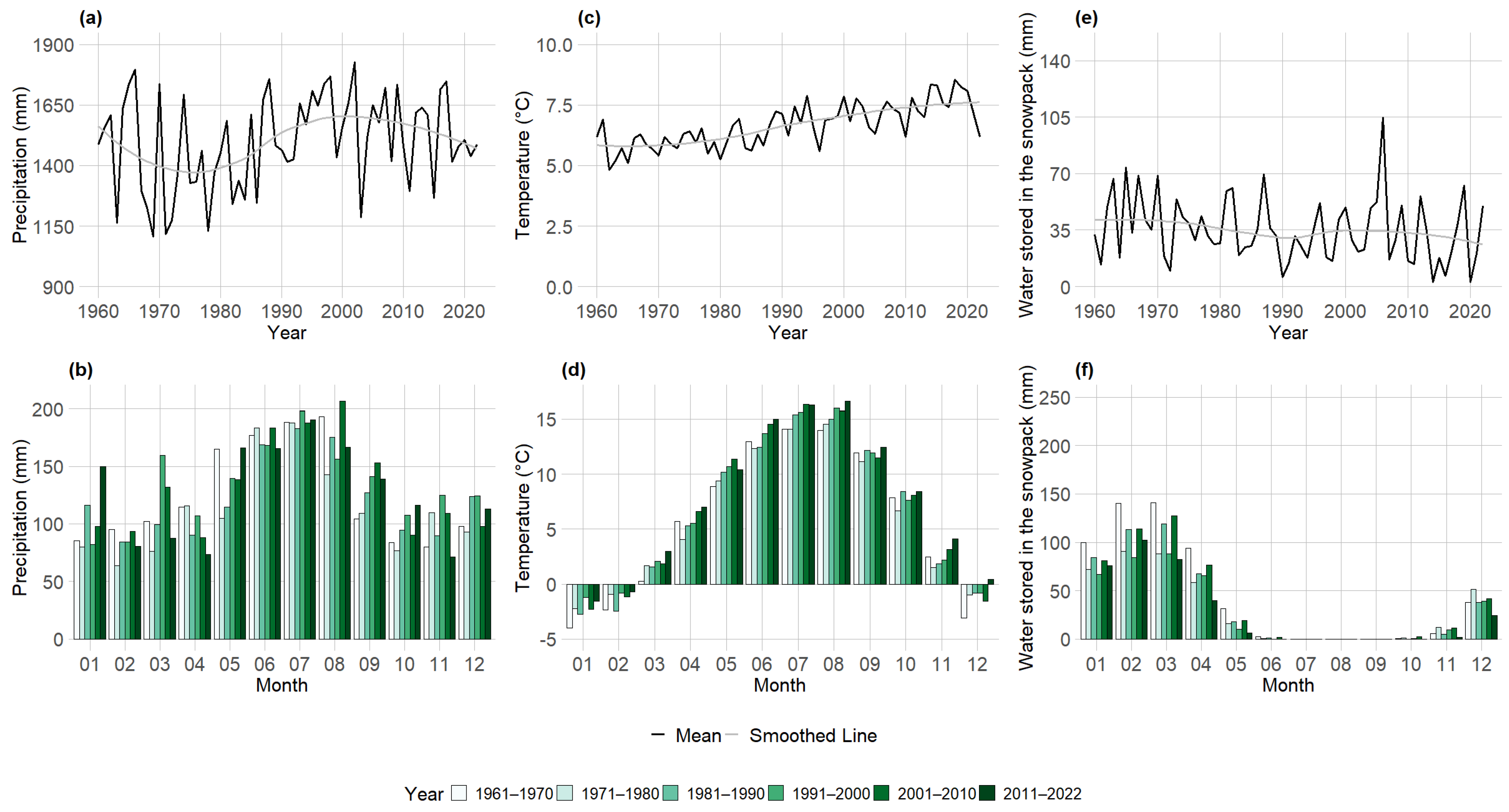
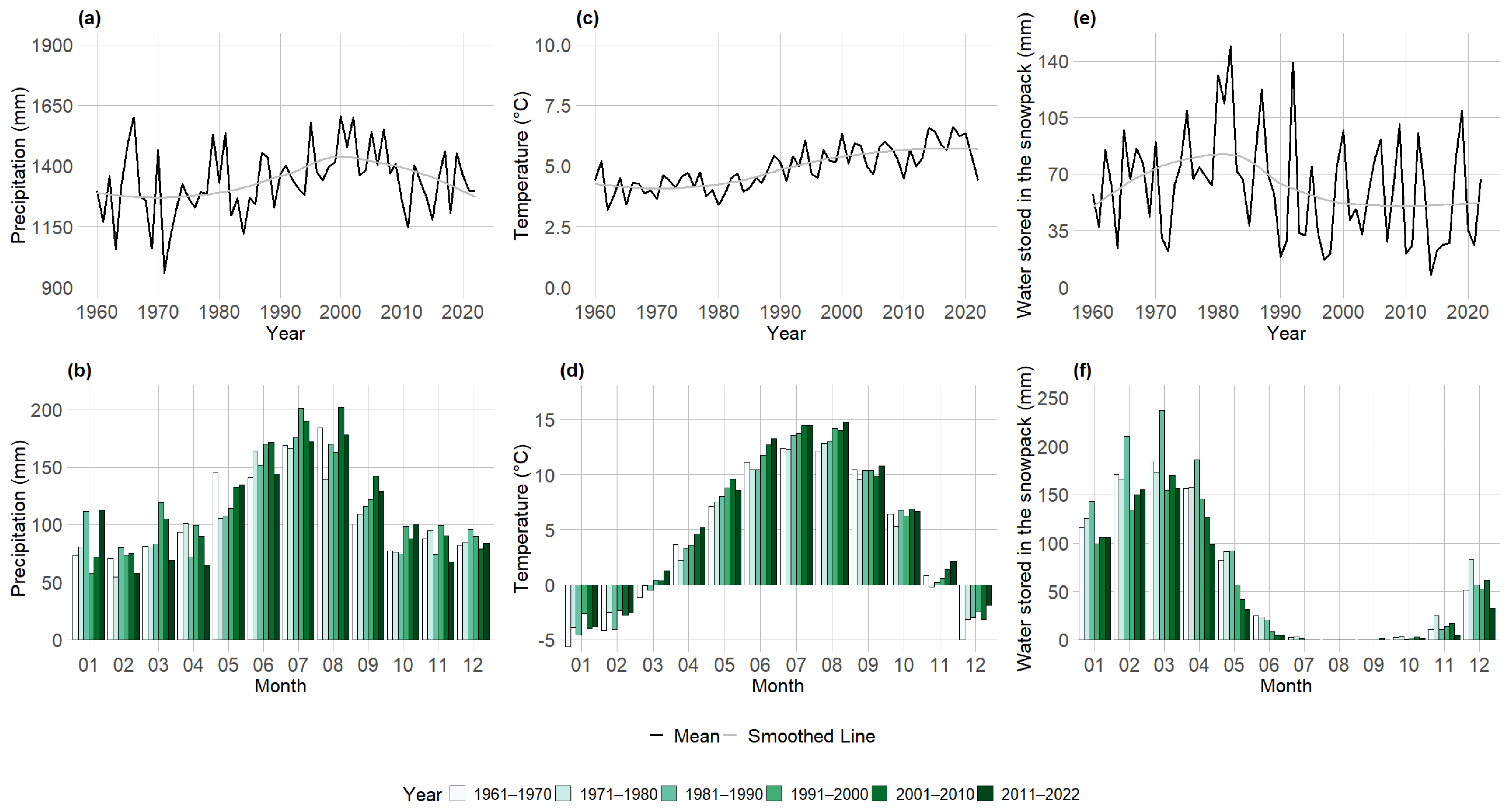
Seasonal precipitation pattern and snow accumulation from 1960 to 2022.
(ii)
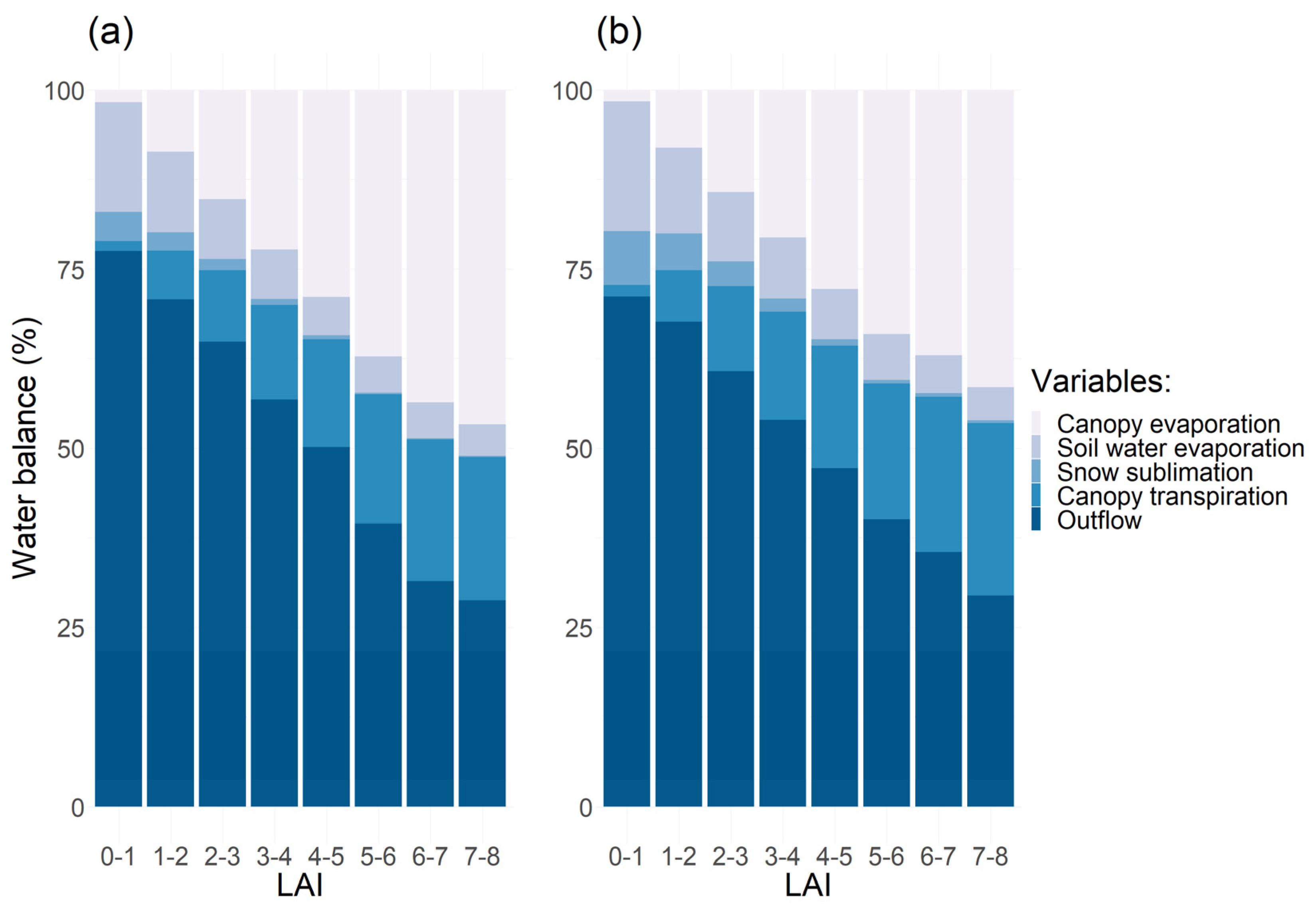
Evapotranspiration, transpiration, and water use efficiency by leaf area index.
(iii)
The water balance of the Norway spruce stands within each catchment.
The novelty of this study is the use of a biogeochemical-mechanistic ecosystem model that integrates the plant–water interactions for assessing the long-term water dynamics of the two different mountain forest catchments growing on different parent materials.

2. Materials and Methods
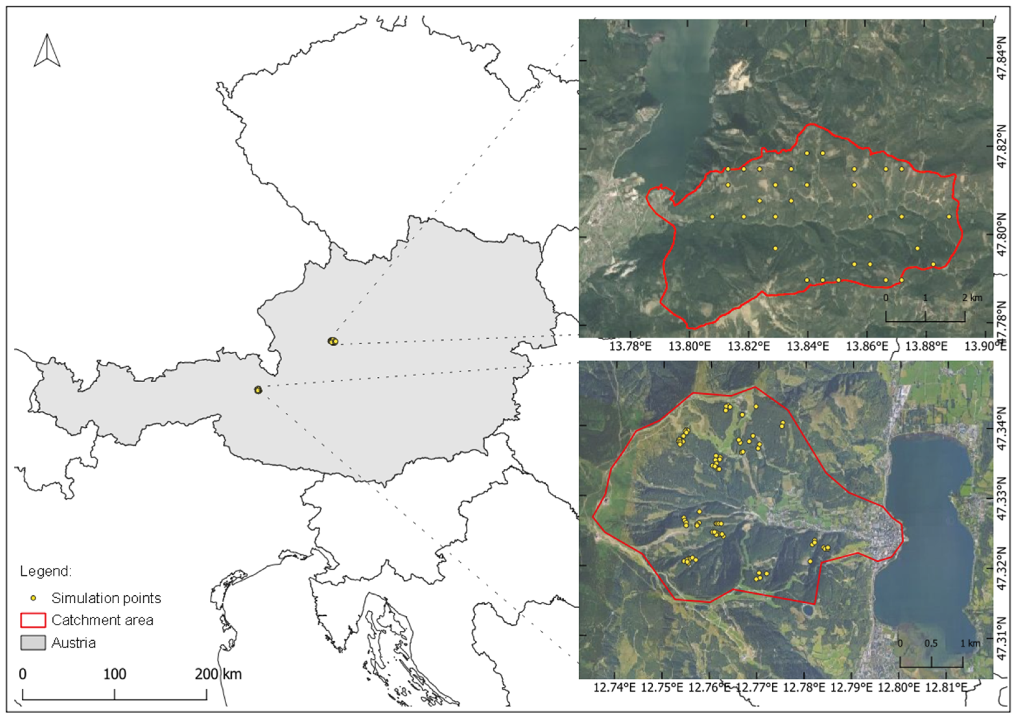
2.1. Study Area

This study was conducted in two distinct geological catchments named Rindbach and Schmittental, located in the Austrian provinces of Upper Austria and Salzburg (Figure 1). The Rindbach watershed, south of the Lak Traunsee, covers an area of 23.4 km2, with a range in elevation from 446 m to 1379 m and in slope between 7.6° to 37.4°. The geology is a so-called “Dachsteinkalk” of the Northern Limestone Alps [16] that consists of moraine, relic, and alluvial origin materials [17]. The dominant soil type, according to the FAO classification, is the Orthic Rendzina, which is formed from calcareous rocks [18]. Between 1960 and 2022, the mean average annual precipitation was 1498 mm, the average annual minimum temperature was 6.7°, the maximum temperature was 16.9°, and the mean average annual temperature was 6.6°.
The Schmittental watershed is drained by the river Schmittenbach and covers an area of 10 km2, with a range in elevation from 924 m to 1690 m and a slope from 25° to 45°. The area is located in the greywacke zone, and the predominant origin materials are moraine, shale, and alluvial materials [17]. The dominant soil types according to the FAO classification are (i) dystric cambisol formed from crystalline rocks and migmatites and (ii) calcific regosols, formed from loamy materials [18]. Between 1960 and 2022, the mean average annual precipitation was 1336 mm, the mean average annual minimum temperature was 6.8°, the maximum temperature was 18.6°, and the mean average annual temperature was 4.9°.
Both watersheds are mainly covered with forests (~60%). However, in the last decades, both areas experienced high rainfall events that affected the water retention and increased the runoff after rainfall. Figure 1 gives an overview of the two catchments, including the location of the 31 forest stands at Rindbach and the 20 forest stands at Schmittental, for which terrestrial data were available.

2.2. Forest Data

The Rindbach watershed covers a typical subalpine northern limestone forest dominated by Norway spruce (Picea abies), with mixtures of silver fir (Albies alba) and common beech (Fagus sylvatica), while Schmittental represents a typical subalpine northern transitional Alpine forest area dominated by Norway spruce with mixtures of silver fir and European larch (Larix decidua). Both watershed areas have experienced a long-lasting management history with occasional catastrophic events, such as bark beetles, avalanches, etc. In both watersheds, about 60% of the total catchment area is covered with forests but was historically much lower due to extensive cattle grazing and pasture farming.
The forestry data were obtained from inventories: (i) The Rindbach data were provided by the Austrian Federal Forest company and (ii) the Schmittental data were collected by the Institute of Silviculture [4]. In both areas, the data recording procedure is consistent with the National Austrian Forest Inventory methods [19], using the angle-count sampling method [20] for tree selection to record the tree height and diameter at breast height (DBH). The summary of the available field data is given in Table 1.

2.3. Biome-BGC Ecosystem Modeling Description and Usage

2.3.1. Model Description

We employed the biogeochemical mechanistic ecosystem model Biome-BGC [14] with its species-specific parameter settings for Norway spruce [15] to simulate the daily carbon, nitrogen, water, and energy flux dynamics within the two watersheds. The model has been applied successfully for several ecosystem studies in central Europe [4,21] and includes a dynamic mortality routine to simulate virgin forests [21], as well as a thinning routine.
The simulation procedure starts with the spin-up or self-initialization routine, using the dynamic mortality routine [21], which mimics natural forest dynamics until a steady state of an assumed undisturbed ecosystem is reached [21]. The simulations require the following input: coordinates, elevation, soil depth, soil texture, current vegetation age and species composition, atmospheric CO2 concentration, nitrogen deposition, and daily weather data. Following the spin-up simulations, the historic land use management such as species composition, management practices (number and duration of rotations), and interventions (planting and thinning) are addressed.
Precipitation enters the model as rainfall (temperature > 0) or as snow (temperature ≤ 0). The calculation of snow sublimation and snow melt considers solar radiation, length of the day, and temperature. If the temperature is below zero, the snow sublimates from the snowpack according to the daily radiation, and if the temperature is higher than zero, snowmelt occurs. The “precipitation route” defines whether the precipitation will be intercepted in the canopy or infiltrate the soil.
The interception rate depends on the leaf area index (LAI) at the plot, the interception coefficient, and the precipitation intensity [14]. The calculation of the projected LAI depends on the total amount of carbon stored in the leaves, the average projected specific leaf area, and the ratio of the all-sided to the projected LAI. The ratio of the all-sided LAI, calculated for the sunlit and shaded canopy fractions, is derived only for plants with leaves.
The intercepted water follows the canopy evaporation process that is limited by the day length. No transpiration is modeled if the length needed to evaporate the canopy water is longer than the day length. If the length needed to evaporate the canopy water is shorter than the day length, the transpiration starts after all the canopy water is evaporated. The water surplus is then directed to the soil.
The evapotranspiration is derived from the Penman–Monteith equation [22] and considers the daylight air temperature, air pressure, vapor pressure deficit, incident shortwave flux density, variables obtained from the meteorological data set, and the variables’ resistance to the water vapor flux and the resistance to sensible heat flux, which were calculated by the model previously to the evapotranspiration calculation.
Canopy evapotranspiration and transpiration are calculated only for trees with leaves and when the day length is < 0. In the model, the calculation runs separately for sun and shade leaves. Transpiration and canopy evaporation calculations consider correction factors applied based on species-specific ecophysiological characterization [15], such as leaf boundary layer and cuticular conductance as a function of the average daylight temperature as well as air pressure. For both calculations, the stomatal conductance, set in the ecophysiological characterization [15], is one of the main drivers. Stomatal conductance is influenced by different multipliers representing the environmental conditions, such as photon flux density, soil water potential, carbon dioxide, vapor pressure deficit, and freezing night temperature. The transpiration is calculated as the multiplication of the Penman–Monteith transpiration, the adjusted day length, and the projected leaf area index [14,15].
The soil holding capacity is calculated according to the pedotransfer function [23,24], which considers the soil depth and soil texture. The soil water potential and the volumetric soil water content are derived according to Cosby et al. [24] and Saxton et al. [25]. Soil water infiltration occurs when the soil water content is neither in the field capacity (−1.5 MPa) nor in the saturation. If these conditions are not reached, the water outflow is assumed.
The simulation process runs on a daily time step, based on meteorological, phenological, ecophysiological, and photosynthetic principles. Within the model, all the processes are connected to generate the ecosystem pools. This study is focused on the dynamics of the soil–water–plant–atmosphere interactions, covering the following output parameters: canopy water evaporation, soil water evaporation, daily evapotranspiration, snow water sublimation, water stored in the snowpack, soil water transpiration, soil water outflow, projected leaf area index, net primary production, and stem carbon.

2.3.2. Simulation Procedure

For the 31 plots dominated by Norway spruce within the Rindbach watershed, the soil texture and soil effective depth were obtained from the European Soil Data Centre (ESDAC) [26,27]. The soil texture parameters sand, silt, and clay were obtained from the “topsoil physical properties of Europe” [26]. Soil depth was obtained from the European soil database [27]. In Schmittental, 20 Norway spruce stands were available, where the soil texture and soil effective depth were obtained from the Austrian National Forest Soil Survey. The species composition and ecophysiological parameter settings are based on Pietsch et al. [15], which present different settings for Norway spruce stands at lower (<1000 m) and higher elevations (>1000 m).
Each simulation with Biome-BGC starts with a “spin up” run, which initializes the model to a steady state [21] using nitrogen deposition, soil depth, and repeated use of the available daily climate data. The nitrogen deposition prior to 1860 is considered as the preindustrial value. From 1860 to 2016 (last available data), nitrogen deposition rates were obtained from the ISIMIP database “https://www.isimip.org (accessed on 1 October 2023)” [28,29]. The annual biological nitrogen fixation was defined as 0.0003 kg N m−2 year−1. Atmospheric CO2 concentration was kept constant at the preindustrial level for the beginning of the simulation (278 ppm) and was continuously increased according to the IPCC’s mean global annual atmospheric CO2 concentration dataset [30].
The model also requires the input of the historic land use and intervention information for each simulation [21]. The historic land use of Rindbach and Schmittental was defined as five (100 years each) and two (of 120 years each) rotations of clear-cut followed by planting, which preceded the current stand situation. In both areas, the species composition during the rotations was defined as Norway spruce. Thinning was applied at ages of 25 and 75 years with a thinning intensity of 20% for Rindbach, and at ages 50 and 70 years with a thinning intensity of 25% for Schmittental.
Daily precipitation and maximum and minimum temperatures for both catchments were obtained from 400 climate stations provided by the Austrian Central Institute for Meteorology and Geodynamics (ZAMG), covering the years 1960 to 2022. This dataset was created using DAYMET, a climate interpolation and simulation tool developed by Thornton et al. [31] and adapted and validated for Austria. The daily weather station records from the ZAMG serve as the input to DAYMET and interpolate and calculate the daily minimum and maximum temperatures, precipitation, solar radiation, and vapor pressure deficit for each point within the two watersheds.
From the precipitation data, the standardized precipitation index (SPI) was calculated according to Edwards and McKeen [32], following a log-logistic (Gamma) distribution function. A period of 3 months (SPI-3) was defined due to its ability to indicate immediate impacts on soil moisture and snowpack.

2.3.3. Validation Procedure

Since the developed parameter settings for Norway spruce [15] were used, model validation was performed according to previous studies [4,15] to justify the regional applicability of the model. Predicted (simulated) stem carbon was converted into tree volume using biomass expansion factors [15] and compared with the tree volume derived from recorded inventory tree data (see Table 1).
Biome-BGC assumes that all the simulated forests are fully stocked. This assumption tends to overestimate the modeled carbon and biomass stocks because forests in central Europe are managed (e.g., thinning, etc.). Management leads to a decline in stand density and reduces stand biomass compared to unmanaged forests. An option to correct for management-induced stand density effects is the calculation of the crown competition factor (CCF) according to Bella [33], which requires open-grown tree dimensions. The ΔV (volume predicted (simulated) vs. volume observed) was calculated, and a logarithmic regression of the ΔV versus CCF including a correlation analysis by catchment was carried out.

3. Results

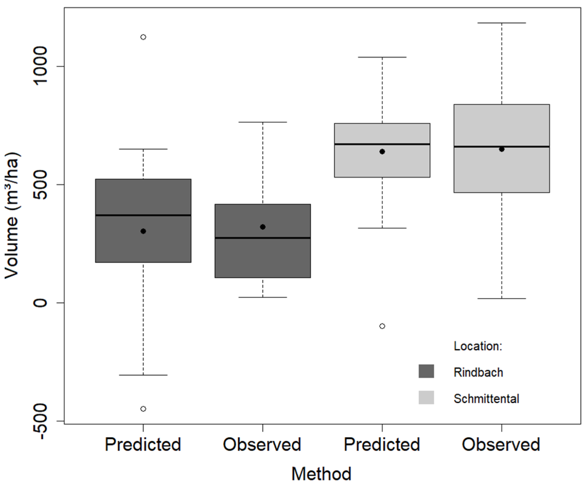
3.1. Model Validation

Any model application has to ensure the reliability of the simulation output. The simulated stem carbon was converted into tree volume and ΔV; the difference between predicted versus observed volume was calculated by catchment and plot. ΔV increased with declining CCF (crown competition factor), suggesting a correction function to address varying stand density. The logarithmic regression of the ΔV versus CCF resulted for Rindbach in a correction function of ΔV = 1164.4 – 208 × ln (CCF), with an R2 = 0.46, and for Schmittental of ΔV = 1239.9 − 237.3 × ln (CCF), with an R2 = 0.23. After applying the correction function for each catchment, the observed values were adjusted to “fully” stocked stands. The results for Rindbach and Schmittental are given in Figure 2.
For Rindbach, the mean predicted and corrected volume revealed 321 m3 ha−1 and the observed volume 304 m3 ha−1. For Schmittental, the corresponding results are 651 m3 ha−1 (predicted corrected volume) and 640 m3 ha−1 (observed volume), indicating that the stocking volume in Schmittental is much higher than in the Rindbach watershed (Figure 2).
The t-test between predicted versus observed volume revealed the following: a t(α=0.05, n=31) = 0.24 for Rindbach and t(α=0.05, n=20) = 0.29 for Schmittental, indicating no significant difference or bias between simulated (predicted) versus observed volume. This suggests that Biome-BGC simulations reveal consistent and unbiased estimates of the flux dynamic parameters for the forests in the two catchments expressed by the precision of the model predictions, which can be also considered as the distribution range of errors. Table 2 provides the statistics including the correlation results by catchment.

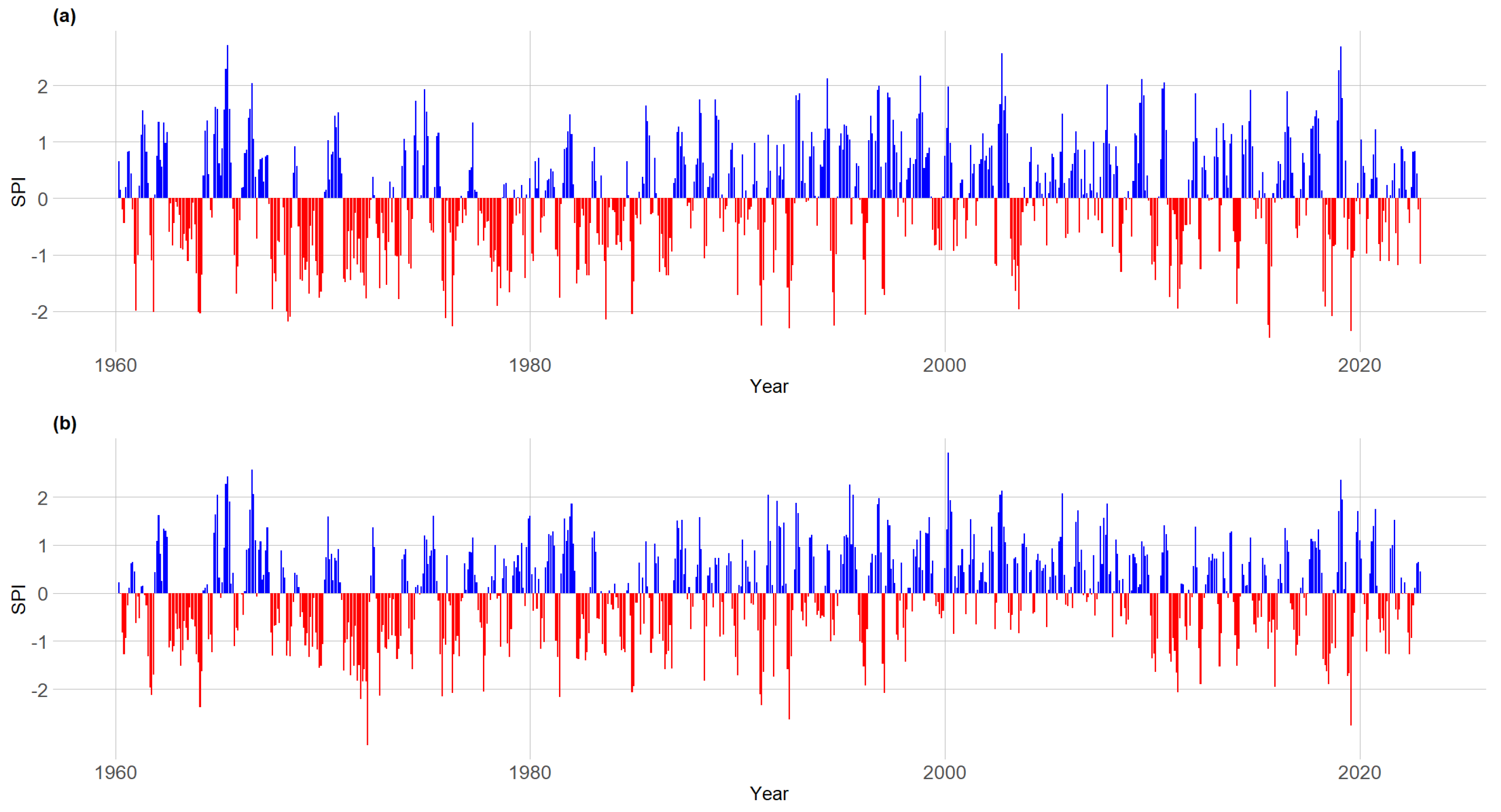
3.2. Seasonal Climate Pattern

The daily climate data from 1960 to 2022 exhibit a mean annual precipitation of 1498 mm for Rindbach and 1336 mm for Schmittental, and no trends in the annual precipitation changed (Figure 3a and Figure 4a). The main precipitation for both catchments occurs during the growing season from May to September. Seasonal temperature patterns are similar in both watersheds (Figure 3d and Figure 4d), with a growing period from April to October, including the warmest months July/August and the coldest months from December to February.
The snow accumulation obtained from Biome-BGC simulations is defined as the water stored in the snowpack. The results show (Figure 3f and Figure 4f) an annual average water stored in the snowpack of 35.1 mm for Rindbach and 62.1 mm for Schmittental, with a declining trend during the last years due to increasing temperatures. The variations within the watersheds result from the elevational range of the simulation points and the associated lower temperatures in higher elevations. This variation was also evident in the seasonal patterns (Figure 3f and Figure 4f). In Schmittental, the snow accumulation took place from October to June, while in Rindbach, the months from November to May accumulated snow, but only half the amount of Schmittental.
Next, the standard precipitation index was calculated for the three-month accumulation period (SPI-3) for the Rindbach and Schmittental forest stands (Figure 5). An SPI below −1.0 indicates a drought increase, whereas an SPI above 1.0 suggests a surplus of rainfall. The index is commonly applied to detect drought stress and allows a comparison between different locations and time periods (Figure 5).

3.3. Plant Water Use and Leaf Area Index

Plant response to the water parameters transpiration, evapotranspiration, and water use efficiency can be associated with the leaf area index—LAI. The mean annual transpiration rates (period 1960 to 2022) increased with increasing LAI (Figure 6) from about 22 mm year−1 for LAI = 1 to > 300 mm year−1 for LAI = 8. The results are similar for Rindbach and Schmittental (Figure 6). The average annual evapotranspiration is also similar but tends to be higher with increasing LAI in Rindbach compared to Schmittental (Figure 6).
The water use efficiency (WUE) calculates the amount of biomass produced per volume of water. In this study, WUE (g C m−2 mm H2O year−1) was calculated based on the net primary production (NPP, kg C m−2 year−1) divided by the evapotranspiration (mm year−1), both parameters were obtained from the Biome-BGC simulations. Concerning the relationship between plant productivity and water use, the water use efficiency (WUE) (see Figure 6) increased with increasing LAI 0–1 to 1–2 for both the Rindbach forests (0.18 to 0.75 g C m−2 mm year−1) and the Schmittental forests (0.16 to 0.62 g C m−2 mm year−1) and reached its peak at an LAI of 2–3 (0.88 g C m−2 mm year−1 for Rindbach and 0.80 g C m−2 mm year−1 for Schmittental) before a slightly declining trend by LAI became evident.

3.4. Impacts of Plant Water Use

Water enters the system by precipitation in the form of rain or snow and is evaporated in the canopy and soil or is needed for transpiration-induced tree growth. Thus, important information in mountainous watersheds is the calculation of the water balance to identify the remaining part of the water inflow (=water outflow), since any water not used on the site will go into water runoff and may cause flooding problems.
The annual simulation results of Biome-BGC were grouped according to the water balance parameters: (i) canopy evaporation, (ii) soil water evaporation, (iii) snow sublimation, (iv) canopy transpiration, and (v) outflow. The summary statistics of the mean values of the water balance parameters for the time period 1960 to 2022 are given in Table 3, and the relative water balance in percent by water balance parameter as well as grouped by leaf area index is shown in Figure 7.

4. Discussion

Daily weather patterns, soil conditions, and forest cover expressed by the leaf area index (LAI) derive the key water cycle parameters such as interception, throughfall, transpiration, as well as runoff (Figure 7). With increasing LAI (Figure 7), the outflow in Rindbach declines from 78% to 29% and from 72% to 31% in Schmittental because more water is used on the forest site. Increasing LAI leads to an increase in canopy evaporation and transpiration from 2% to 47% and 1.5% to 20%, respectively, in Rindbach, and from 2% to 40% (LAI) and 1.7% to 24% (canopy evaporation) in Schmittental (Figure 7).
The amount of runoff and its frequency are important to avoid flooding or mudslides, which are a serious threat to housing areas and infrastructure in mountainous areas [4,5]. However, water cycle parameters are strongly affected by the energy, nutrient, and growth potential of forests, and related field measurements along these processes are difficult to obtain. Thus, the biogeochemical-mechanistic model Biome-BGC was employed [14] with its species-specific parameter settings for the Norway spruce [15] to cover the flux dynamics including the water cycle parameters of forest ecosystems. The model validation prior to our analysis revealed unbiased and consistent simulation runs (Figure 2), since no significant differences between predicted versus observed volume for the 31 forests stands at Rindbach (t = 0.23n.s. < t(α=0.05, n−1=30) = 2.04) and the 20 stands at Schmittental t = 0.29 < t(α=0.05, n−1=19) = 2.53) were detectable. Note that the observed forest data for stand density expressed by the CCF (crown competition factor) were corrected according to Bella [33] to address the fact that the forest sites within the catchments experienced some common forest management, while the Biome-BGC simulations assume fully stocked stands. With this adjustment, the model limitation in simulating only fully stocked stands was corrected.
A limitation of flux models such as Biome-BGC, is that the mixture effects of forest stands are difficult or even impossible to model since the general modeling approach is based on a pool simulation of the key processes (energy, water, nitrogen, and carbon) and does not address individual tree growth within a forest stand [14,15]. Since these key ecophysiological processes are species-specific [15], mixture effects within forest stands resulting from competition for resources among tree species are difficult to model.
Distinct geological conditions and the differences in mean stand age (Table 1) result in different volume stocks. As shown in Figure 2, the Rindbach forests exhibit about half of the average stocking volume with 304 m3 ha−1, compared to the Schmittental forests with 651 m3 ha−1. The Rindbach sites are orthic rendzina, characterized by a moderately developed and shallow soil profile, while the Schmittental sites consist of cambisol with a well-developed soil profile originating from mineral-rich parent materials. This leads to differences in soil textures, soil drainage, productivity, and higher drought sensitivity of Norway spruce compared to deep, silty soil [7].
Plant growth, and thus the related water cycle parameters, are also influenced by climate variables and elevation. The Rindbach catchment forest area ranges from 466 m to 1379 m in elevation, compared to Schmittental with a range from 924 m to 1690 m (Table 1). For the period 1960 to 2022, the two catchments of our analysis exhibited similar annual average precipitation rates with 1498 mm for Rindbach and 1336 for Schmittental, while the average annual temperatures differed by 1.7 °C degrees (e.g., Rindbach with 6.6 °C compared to Schmittental with 4.9 °C). This leads to differences in the average amount of water stored as snowpack, which was almost twice as much at Schmittental, compared to Rindbach (see Figure 3 and Figure 4). This suggests that a higher continuous water supply from snowmelt can be expected, promoting forest growth in Schmittental.
A previous study of a Swedish forest watershed [34] covering the same period as our study showed that the main limiting factors for Norway spruce growth vary according to the altitude, with low temperatures being the main limiting factor at high altitudes and precipitation or moisture being critical in lower altitudes. Even though higher temperatures lead to a longer growing season, the higher frequency of drought events will result in higher susceptibility to bark beetles, which negatively influence productivity [3].
The plant–water relations expressed as leaf area index (LAI) versus evaporation, transpiration, and water use efficiency (Figure 6) are similar within both catchments—Rindbach and Schmittental. As expected, the development is strongly related to LAI, emphasizing the importance of crown cover to control the water cycle processes. At a low LAI of ≤ 3 m2 m−2 (Figure 6), the soil exposure and solar energy reaching the forest floor are high and contribute to increasing the fractions of soil evaporation. With forest canopy closure and an increase in litterfall, the contribution of soil evaporation and outflow decreases [4], but the increase in LAI results in an increase in the relative proportion of canopy evaporation and transpiration, reducing the proportion of water outflow (Figure 7). The water balance effects are similar in both catchments (Figure 7) and confirm previous studies within Norway spruce stands from central Sweden with 39% evapotranspiration [34].
Increasing transpiration leads to an increase in water use efficiency (WUE), i.e., the rate of carbon assimilation versus transpiration. Within both catchments, the water use efficiency increases with increasing LAI (Figure 6) and reaches a peak at an LAI of 2–3, slightly declining before it remains more or less constant at an LAI > 4. Note that a low LAI (e.g., <3—Figure 6) may result from a young forest that has not yet reached a full crown cover or has a low stand density, which both affect the water cycle parameters within a forest stand [4].

5. Conclusions

Forests are important for the water dynamics of mountainous areas. Commonly, mountain forests in central Europe have enough rain, and higher outflow rates are often associated with flooding and mudslides causing damage to the infrastructure. Thus, if more water is evaporated and transpired, less water goes into outflow and we can expect that even during excess rain events, less damage occurs. From a forest management perspective, it is important to ensure stable sustainable forests with a high leaf area index. As shown in the simulation study, the increase in leaf area index resulted in a decline of approximately 49% and 41% of the outflow for Rindbach and Schmittental, confirming the importance of forest cover in reducing outflow and enhancing the protective function of mountainous forests.
An Important concern is the impact of climate change on the water balance of mountainous catchments. From the recorded data it is evident that the average precipitation may remain stable, but with an increase in temperature, the form of precipitation may change (more rain and less snow), and this may have a severe impact on a continued water supply due to snow melt. For the two catchments, the total precipitation (rain and snow) remained constant, while the mean annual temperature increased by 1.9 °C in Rindbach, compared to 1.6 °C at Schmittental, indicating that the snow accumulation declined at Rindbach. Considering the fact that the parent material in Rindbach is a limestone area (“Dachsteinkalk”) with high porosity and very good water drainage, compared to Schmittental, which is located in the greywacke zone with less water drainage, it can be expected that drought stress has a higher risk at Rindbach compared to Schmittental. This is crucial because this may reduce the resilience of mountain forest ecosystems and enhance the susceptibility to further damage such as bark beetle infections and forest fires.

Author Contributions

Conceptualization, F.d.B. and H.H.; methodology, F.d.B.; software, F.d.B.; validation, F.d.B.; formal analysis, F.d.B.; investigation, F.d.B. and H.H.; resources, F.d.B.; data curation, F.d.B.; writing—original draft preparation, F.d.B.; writing—review and editing, H.H.; visualization, F.d.B.; supervision, H.H.; project administration, H.H.; funding acquisition, H.H. All authors have read and agreed to the published version of the manuscript.

Funding

This research was funded by the Austrian Ministry of Agriculture, Forestry, Regions, and Water Management under the “Waldfonds” program and is part of the activity entitled Initial compilation of areal site data in a forestry dominated torrential headwater catchment as a basis for an integral catchment management.

Data Availability Statement

The data presented in this study are available on request from the corresponding author.

Acknowledgments

We thank Hellen David from the Austrian Federal Forest Company (öbf) for making the Rindbach inventory data available.

Conflicts of Interest

The authors declare no conflicts of interest.

References

  1. Myhre, G.; Alterskjær, K.; Stjern, C.W.; Hodnebrog, Ø.; Marelle, L.; Samset, B.H.; Sillmann, J.; Schaller, N.; Fischer, E.; Schulz, M.; et al. Frequency of Extreme Precipitation Increases Extensively with Event Rareness under Global Warming. Sci. Rep. 2019, 9, 16063. [Google Scholar] [CrossRef]
  2. Schmid, U.; Frehner, M.; Glatthorn, J.; Bugmann, H. ProForM: A Simulation Model for the Management of Mountain Protection Forests. Ecol. Model. 2023, 478, 110297. [Google Scholar] [CrossRef]
  3. Price, M.F.; Gratzler, G.; Duguma, L.A.; Kohler, T.; Maselli, D.; Romeo, R. Mountain Forests in a Changing World—Realizing Values, Addressing Challenges; FAO with the support of the Swiss Agency for Development and Cooperation, SDC; Food and Agriculture Organization of the United Nations: Roma, Italy, 2011. [Google Scholar]
  4. Pötzelsberger, E.; Hasenauer, H. Forest–Water Dynamics within a Mountainous Catchment in Austria. Nat. Hazards 2015, 77, 625–644. [Google Scholar] [CrossRef]
  5. Scheidl, C.; Heiser, M.; Kamper, S.; Thaler, T.; Klebinder, K.; Nagl, F.; Lechner, V.; Markart, G.; Rammer, W.; Seidl, R. The Influence of Climate Change and Canopy Disturbances on Landslide Susceptibility in Headwater Catchments. Sci. Total Environ. 2020, 742, 140588. [Google Scholar] [CrossRef] [PubMed]
  6. Caudullo, G.; Tinner, W.; de Rigo, D. Picea Abies in Europe: Distribution, Habitat, Usage and Threats. In European Atlas of Forest Tree Species; San-Miguel-Ayanz, J., de Rigo, D., Caudullo, G., Houston Durrant, T., Mauri, A., Eds.; Publication Office of the European Union: Luxembourg, 2016. [Google Scholar]
  7. Rehschuh, R.; Mette, T.; Menzel, A.; Buras, A. Soil Properties Affect the Drought Susceptibility of Norway Spruce. Dendrochronologia 2017, 45, 81–89. [Google Scholar] [CrossRef]
  8. Cavalli, J.P.; Reichert, J.M.; Rodrigues, M.F.; de Araújo, E.F. Composition and Functional Soil Properties of Arenosols and Acrisols: Effects on Eucalyptus Growth and Productivity. Soil Tillage Res. 2020, 196, 104439. [Google Scholar] [CrossRef]
  9. Hümann, M.; Schüler, G.; Müller, C.; Schneider, R.; Johst, M.; Caspari, T. Identification of Runoff Processes—The Impact of Different Forest Types and Soil Properties on Runoff Formation and Floods. J. Hydrol. 2011, 409, 637–649. [Google Scholar] [CrossRef]
  10. Sun, G.; Wei, X.; Hao, L.; Sanchis, M.G.; Hou, Y.; Yousefpour, R.; Zhang, Z. Forest Hydrology Modeling Tools for Watershed Management: A Review. For. Ecol. Manag. 2023, 530, 120755. [Google Scholar] [CrossRef]
  11. Arnold, J.G.; Srinivasan, R.; Muttiah, R.S.; Williams, J.R. Large Area Hydrologic Modeling and Assessment Part I: Model Development. J. Am. Water Resour. Assoc. 1998, 34, 73–89. [Google Scholar] [CrossRef]
  12. Šimůnek, J.; Šejna, M.; Saito, H.; Sakai, M.; van Genuchten, M.T. The HYDRUS-1D Software Package for Simulating the One-Dimensional Movement of Water, Heat, and Multiple Solutes in Variably-Saturated Media; University of California Riverside: Riverside, CA, USA, 2008. [Google Scholar]
  13. Thornton, P.E.; Law, B.E.; Gholz, H.L.; Clark, K.L.; Falge, E.; Ellsworth, D.S.; Goldstein, A.H.; Monson, R.K.; Hollinger, D.; Falk, M.; et al. Modeling and Measuring the Effects of Disturbance History and Climate on Carbon and Water Budgets in Evergreen Needleleaf Forests. Agric. For. Meteorol. 2002, 113, 185–222. [Google Scholar] [CrossRef]
  14. White, M.A.; Thornton, P.E.; Running, S.W.; Nemani, R.R. Parameterization and Sensitivity Analysis of the BIOME-BGC Terrestrial Ecosystem Model: Net Primary Production Controls. Earth Interact. 2000, 4, 1–84. [Google Scholar] [CrossRef]
  15. Pietsch, S.A.; Hasenauer, H.; Thornton, P.E. BGC-Model Parameters for Tree Species Growing in Central European Forests. For. Ecol. Manag. 2005, 211, 264–295. [Google Scholar] [CrossRef]
  16. Rupp, C.; Linner, M.; Mandl, G.W. Geologische Karte von Oberösterreich; Geologische Bundesanstalt: Vienna, Austria, 2011. [Google Scholar]
  17. Federal Research and Training Center for Forests, Natural Hazards and Landscape (BFW). “eBOD”—Digital Soil Map of Austria; BFW: Vienna, Austria, 2023. [Google Scholar]
  18. Umweltbundesamt GmbH. BORIS—Bodeninformationssystem; Umweltbundesamt GmbH: Dessau-Roßlau, Germany, 2023. [Google Scholar]
  19. Gabler, K.; Schadauer, K. Methods of the Austrian Forest Inventory 2000/0—Origins, Approaches, Design, Sampling, Data Models, Evaluation and Calculation of Standard Error; BFW: Vienna, Austria, 2008. [Google Scholar]
  20. Bitterlich, W. Die Winkelzählprobe. Allg. Forst Holzwirtsch. 1948, 59, 4–5. [Google Scholar] [CrossRef]
  21. Pietsch, S.A.; Hasenauer, H. Evaluating the Self-Initialization Procedure for Large-Scale Ecosystem Models. Glob. Change Biol. 2006, 12, 1658–1669. [Google Scholar] [CrossRef]
  22. Allen, R.G.; Pereira, L.S.; Raes, D.; Smith, M. Crop Evapotranspiration—Guidelines for Computing Crop Water Requirements—FAO Irrigation and Drainage Paper 56; FAO—Food and Agriculture Organization of the United Nations: Roma, Italy, 1998. [Google Scholar]
  23. Clapp, R.B.; Hornberger, G.M. Empirical Equations for Some Soil Hydraulic Properties. Water Resour. Res. 1978, 14, 601–604. [Google Scholar] [CrossRef]
  24. Cosby, B.J.; Hornberger, G.M.; Clapp, R.B.; Ginn, T.R. A Statistical Exploration of the Relationships of Soil Moisture Characteristics to the Physical Properties of Soils. Water Resour. Res. 1984, 20, 682–690. [Google Scholar] [CrossRef]
  25. Saxton, K.E.; Rawls, W.J.; Romberger, J.S.; Papendick, R.I. Estimating Generalized Soil-Water Characteristics from Texture. Soil Sci. Soc. Am. J. 1986, 50, 1032–1036. [Google Scholar] [CrossRef]
  26. Ballabio, C.; Panagos, P.; Monatanarella, L. Mapping Topsoil Physical Properties at European Scale Using the LUCAS Database. Geoderma 2016, 261, 110–123. [Google Scholar] [CrossRef]
  27. Hiederer, R. Mapping Soil Typologies—Spatial Decision Support Applied to the European Soil Database; European Commission: Luxembourg, 2013. [Google Scholar] [CrossRef]
  28. Lamarque, J.F.; Dentener, F.; McConnell, J.; Ro, C.U.; Shaw, M.; Vet, R.; Bergmann, D.; Cameron-Smith, P.; Dalsoren, S.; Doherty, R.; et al. Multi-Model Mean Nitrogen and Sulfur Deposition from the Atmospheric Chemistry and Climate Model Intercomparison Project (ACCMIP): Evaluation of Historical and Projected Future Changes. Atmos. Chem. Phys. 2013, 13, 7997–8018. [Google Scholar] [CrossRef]
  29. Tian, H.; Yang, J.; Lu, C.; Xu, R.; Canadell, J.G.; Jackson, R.B.; Arneth, A.; Chang, J.; Chen, G.; Ciais, P.; et al. The Global N2O Model Intercomparison Project. Bull. Am. Meteorol. Soc. 2018, 99, 1231–1251. [Google Scholar] [CrossRef]
  30. Enting, I.G.; Wigley, T.M.L.; Heimann, M. Future Emissions and Concentrations of Carbon Dioxide: Key Ocean/Atmosphere/Land Analyses; CSIRO: Brisbane City, QLD, Australia, 1994. [Google Scholar]
  31. Thornton, P.E.; Running, S.W.; White, M.A. Generating Surfaces of Daily Meteorological Variables over Large Regions of Complex Terrain. J. Hydrol. 1997, 190, 214–251. [Google Scholar] [CrossRef]
  32. Edwards, D.C.; McKee, T.B. Characteristics of 20th Century Drought in the United States at Multiple Time Scales; Climatology Report Number 97-2; Colorado State University: Fort Collins, CO, USA, 1997. [Google Scholar]
  33. Bella, I.E. A New Competition Model for Individual Trees. For. Sci. 1971, 17, 364–372. [Google Scholar]
  34. Hasper, T.B.; Wallin, G.; Lamba, S.; Hall, M.; Jaramillo, F.; Laudon, H.; Linder, S.; Medhurst, J.L.; Räntfors, M.; Sigurdsson, B.D.; et al. Water Use by Swedish Boreal Forests in a Changing Climate. Funct. Ecol. 2016, 30, 690–699. [Google Scholar] [CrossRef]
Figure 1. The catchment areas (red line) Rindbach and Schmittental located in the Austrian provinces Upper Austria and Salzburg with the location of the available forest stands (yellow dots) and the geographic coordinates (WGS 84). The two watersheds are mainly covered with subalpine Norway spruce forests and differ in the geological parent material. At Rindbach, it is the so-called “Dachsteinkalk” of the Northern Limestone Alps, and at Schmittental, it is the greywacke zone with moraine, shale, and alluvial material.
Forests 15 00035 g001
Figure 2. Mean predicted (simulated with Biome-BGC) and the corrected observed volume/ha including the range of 31 plots at Rindbach and the 20 plots at Schmittental forest stands. Solid circles represent the mean values, while hollow circles represent the outliers.
Forests 15 00035 g002
Figure 3. Annual and seasonal patterns of the climate variables precipitation (a,b), temperature (c,d), and water stored in the snowpack (e,f) for the Rindbach watershed. The annual patterns represent the yearly mean for the 31 plots evaluated in the Rindbach watershed. The smoothed line was generated with Locally Weighted Scatterplot Smoothing, a non-parametric method that fits a smooth curve through the data by giving more weight to nearby data points and less weight to distant points. The seasonal pattern represents the monthly mean among the 31 plots in 10 years.
Forests 15 00035 g003
Figure 4. Annual and seasonal patterns of the climate variables precipitation (a,b), temperature (c,d), and water stored in the snowpack (e,f) for the Schmittental watershed. The annual patterns represent the yearly mean for the 20 plots monitored in the Schmittental watershed. The smoothed line was generated with Locally Weighted Scatterplot Smoothing, a non-parametric method that fits a smooth curve through the data by giving more weight to nearby data points and less weight to distant points. The seasonal pattern represents the monthly mean among the 20 plots in 10 years.
Forests 15 00035 g004
Figure 5. Standardized precipitation index (SPI) computed for a three-month accumulation period for the Rindbach (a) and Schmittental (b) forest stands. The time period ranges from 1960 to 2022.
Forests 15 00035 g005
Figure 6. Annual variation in the transpiration, evapotranspiration, and water use efficiency for different leaf area index (LAI) groups. The results show the mean by group for the 31 plots at Rindbach and the 20 plots at Schmittental, covering the period 1960 to 2022.
Forests 15 00035 g006
Figure 7. Relative proportion of the average annual water balance parameters simulated for the forest stands in Rindbach (a) and Schmittental (b) covering the period 1960 to 2022. The water balance parameters are canopy evaporation, soil water evaporation, snow sublimation, canopy transpiration, and outflow grouped by leaf area index (LAI).
Forests 15 00035 g007
Table 1. Summary statistics of the available field data for the catchment Rindbach and Schmittental, covering elevation, stand age, diameter at breast height (DBH) tree height, volume, basal area (BA), stem number per hectare (N/ha), and crown competition factor (CCF) of the Norway spruce stands. Min. and Max. are the minimum and maximum of the data, sd is the standard deviation of the mean value (Mean), and N is the number of plots available for each catchment.
Stand CharacteristicsRindbach N = 31 PlotsSchmittental N = 20 Plots
Min.Max.MeansdMin.Max.Meansd
Elevation (m)46613791027200.492416901370212.1
Stand age (years)121776642272358441
DBH (cm)14.969.830.713.911.354.733.710.7
Tree height (m)4.333.516.66.06.741.527.88.0
Volume (m3/ha)21.8766304218.716.81184.9640277.5
BA (m2/ha)5.086.041.725.34.088.057.416.9
N/ha20.82704.31005784.185.57915.312961332.8
CCF (%)13.0481.3204139.429.41073.3349161.9
Table 2. Correlation analysis between predicted versus observed volume for the 31 plots at Rindbach and the 20 plots at Schmittental forest stands.
LocationInterceptRegression CoefficientsStandard Error of EstimatesCorrelation CoefficientF-Valueα
Rindbach190.630.35191.50.269.54<0.01
Schmittental130.910.80233.040.2728.11<0.01
Table 3. Annual minimum, maximum mean, and standard deviation (sd) of the water balance parameters canopy evaporation, soil water evaporation, snow sublimation, transpiration, and outflow simulated for the period 1960 to 2022 for the Rindbach and Schmittental forest stands.
Variable (mm Year−1)MinimumMaximumMeansd
Rindbach
Canopy evaporation (mm/year)5.0971.2501.5214.1
Soil water evaporation (mm/year)18.6313.896.250.9
Snow sublimation (mm/year)0.0171.410.719.4
Transpiration (mm/year)4.5361.8243.587.7
Outflow (mm/year)42.51874.3645.6286.2
Schmittental
Canopy evaporation (mm/year)4.3873.1402.5161.2
Soil water evaporation (mm/year)16.9307.396.349.5
Snow sublimation (mm/year)0.2264.917.128.9
Transpiration (mm/year)4.2394.8239.784.5
Outflow (mm/year)113.61480.5582.0207.1
Disclaimer/Publisher’s Note: The statements, opinions and data contained in all publications are solely those of the individual author(s) and contributor(s) and not of MDPI and/or the editor(s). MDPI and/or the editor(s) disclaim responsibility for any injury to people or property resulting from any ideas, methods, instructions or products referred to in the content.

