Estimating Forest Variables for Major Commercial Timber Plantations in Northern Spain Using Sentinel-2 and Ancillary Data

Abstract

In this study, we used Spanish National Forest Inventory (SNFI) data, Sentinel-2 imagery and ancillary data to develop models that estimate forest variables for major commercial timber plantations in northern Spain. We carried out the analysis in two stages. In the first stage, we considered plots with and without sub-meter geolocation, three pre-processing levels for the Sentinel-2 images and two machine learning algorithms. In most cases, geometrically, radiometrically, atmospherically and topographically (L2A-ATC) corrected images and the random forest algorithm provided the best results, with topographic correction producing a greater gain in model accuracy as the average slope of the plots increased. Our results did not show any clear impact of the geolocation accuracy of SNFI plots on results, suggesting that the usual geolocation accuracy of SNFI plots is adequate for developing forest models with data obtained from passive sensors. In the second stage, we used all plots together with L2A-ATC-corrected images to select five different groups of predictor variables in a cumulative process to determine the influence of each group of variables in the final RF model predictions. Yield variables produced the best fits, with R² ranging from 0.39 to 0.46 (RMSE% ranged from 44.6% to 61.9%). Although the Sentinel-2-based estimates obtained in this research are less precise than those previously obtained with Airborne Laser Scanning (ALS) data for the same species and region, they are unbiased (Bias% was always below 1%). Therefore, accurate estimates for one hectare are expected, as they are obtained by averaging the values of 100 pixels (model resolution of 10 m pixel⁻¹) with an expected error compensation. Moreover, the use of these models will overcome the temporal resolution problem associated with the previous ALS-based models and will enable annual updates of forest timber resource estimates to be obtained.

1. Introduction

The role of forest plantations in helping to tackle many of the great challenges of our time is increasingly recognized, as forests provide goods and services, generate jobs, sustain incomes and act as a source of food and fuel [1]. Moreover, new value-added products obtained from these forest resources (e.g., lignocellulosic biofuels, cellulose-based fibers such as viscose, and the multitude of valuable substances obtained from forest residues in biorefineries) indicate the increasing importance of forest plantations to society as alternative renewable sources for producing bioenergy, biochemicals and biomaterials [2]. Northern Spain (which encompasses the regions of Galicia, Asturias, Cantabria and the Basque Country) is one of the most productive forest areas in Europe and is covered by extensive plantations of maritime pine, radiata pine and Tasmanian blue gum. Thus, in the period 2005–2019, the average harvested volume of the three cited species reached 9,700,505 m³ year⁻¹, which represented 89.9% of the total volume harvested annually (TVHA) in the four regions and 63.3% of the TVHA in the whole of Spain [3]. These data highlight the great socioeconomic dimension of the forest plantations, which also provide other important ecosystem services, including wildlife refuge provision, climate change mitigation and hydrological regulation. Quantification of forest variables, particularly current timber stocks (in terms of volume, biomass or carbon), and of their distribution and temporal variation over the territory, is therefore essential to facilitate planning for landowners, enterprises, forest managers and researchers.

Evaluation of forest resources has traditionally been based on measurement of the diameter at breast height and total height of the trees in numerous plots (direct method), and remains to be the most common method for estimating forest stocks [4]. Although this method is accurate, it is expensive, time-consuming and presents operational problems as it can only be applied to small areas [5]. However, the plot-level data can also be used as “training data” to develop forest models based on variables determined by remote sensing (indirect method) [6].

The combined use of public databases (e.g., the National Forest Inventory, NFI) and the semi-automatic capture of state variables by various remote sensing techniques has enabled these problems to be overcome and forest models to be developed without the need for fieldwork [7]. In fact, timber stock quantification is currently one of the most common applications of remote sensing (RS) and thus supports sustainable forest management, as RS provides reliable data and overcomes the two aforementioned limitations of traditional methods (data scarcity and operational problems), providing estimates even in areas not previously sampled [8].

Depending on whether the energy to which the sensors respond is internal or external to the system, remote sensing can be classified into two groups: (i) active and (ii) passive. In the first group, the sensor emits energy and then detects and measures the energy reflected from the target, while in the second, the sensor measures the external solar energy reflected from the Earth’s surface (surface reflectance or reflectance) [9] using optical multispectral or hyperspectral sensors. Airborne Laser Scanning (ALS) (also referred to as LiDAR: Light Detection and Ranging) and, to a lesser extent, RADAR (Radio Detection and Ranging) are the active sensing methods most commonly used for forestry applications. Active sensors can penetrate the forest canopy and do not depend on weather, cloud or lighting conditions [10]. As a result of their greater accuracy and higher spatial resolution, these types of sensors are frequently used to study the vertical structure of forests [11,12] and timber volume or biomass (e.g., [13,14]). However, they provide predictions with low temporal resolution. Since 2008, Spain has had available a national ALS coverage compiled by the PNOA-LiDAR project of the Instituto Geográfico Nacional (IGN) [15]. Although this database is very valuable for forestry purposes, it has several drawbacks: (i) low temporal resolution and (ii) different data acquisition depending on the region. Although the temporal resolution of the ALS data is officially 5 years, delays often occur, leading to intervals of up to 8 years in some regions (e.g., Asturias 1st coverage 2012 and 2nd in 2020). With such long intervals, forest stock estimation quickly becomes out of date because the species used are fast growing and also because of the occurrence of abiotic/biotic damage, forest fires and forestry management actions (clearcutting or thinning). Different rates of data acquisition in different regions also generate problems associated with lack of harmonization when building models for several nearby regions [14].

These two drawbacks of ALS data can be overcome by using passively, remotely sensed data with very high temporal resolution. Although data from passive sensors are limited by cloud cover, the short revisit period of satellites increasingly facilitates production of cloud-free mosaics, even within short periods of time [16].

The free availability of remotely sensed data (e.g., Landsat, MODIS or Sentinel) has led to a great increase in the use of this type of data in the last decade for estimating several forest variables such as growing stock volume [4,17], biomass [18,19], forest cover [16,20] and forest changes [21]. The Sentinel-2A and Sentinel-2B satellites, launched by the European Space Agency (ESA) through its Copernicus program in 2015 (S2A) and 2017 (S2B), have a temporal resolution of five days, and the imagery includes 13 spectral bands with a spatial resolution ranging from 10, 20 and 60 m/pixel depending on the band [22]. The high levels of temporal and spatial resolution have enabled estimation of forest variables with sufficient spatial detail for forest inventories and sustainable forest management purposes [17] and have made these images a popular source of remotely sensed data for forestry research in recent years [23].

Public databases such as National Forest Inventories (NFIs) include information about key forest variables (structure, growth and yield) and provide the field data necessary to construct wall-to-wall spatial models to predict forest variables using remote sensing data as independent variables. However, the major problems associated with the combined use of NFI and remotely sensed data are the temporal mismatches and the low positioning accuracy of the NFI field plots that sometimes occur. The first is not a problem when using optical data from Sentinel-2, Landsat-8 or MODIS because of the high temporal resolution of these sensors. However, the second has been recognized to have important effects on forest variable estimation, mainly when dealing with LiDAR data [24]. This has led researchers to adopt different approaches in an attempt to mitigate the effects (e.g., [4,14,25]).

Both parametric and nonparametric models have frequently been used to derive forest stock variables from remotely sensed data (e.g., [18,26]). The main advantages of parametric linear models are their simplicity and clarity, while the main drawbacks are the probability of selecting highly correlated predictors with little physical justification and the nonfulfilment of the assumptions of normality, homoscedasticity, independence and linearity [27]. Unlike linear models, machine learning algorithms can learn highly complex nonlinear relationships, integrate multiple factors and thus obtain better simulation results [10]. However, the resulting models are usually complex, and the role of the variables selected from the models may be difficult to understand [28].

In this study, we evaluated the use of multispectral Sentinel-2 imaginary to solve the problem of low temporality in previous models obtained from ALS data for the same species in northern Spain. The main objective of this study was to generate, for major commercial timber plantations in northern Spain, a high-resolution raster database with information about key forest variables based on Sentinel-2 images. To fulfil the main objective, the specific objectives were as follows: (i) generation of a high-resolution raster database including the independent variables considered in this study; (ii) testing the effect on predictions of implementing different image correction levels and/or plot geolocation accuracy and by using different categories of independent variables; (iii) selection of the best empirical model by comparing two well-known nonparametric machine learning regression techniques; and (iv) use of the best approach to generate a high-resolution raster database including key forest variables.

2. Materials and Methods

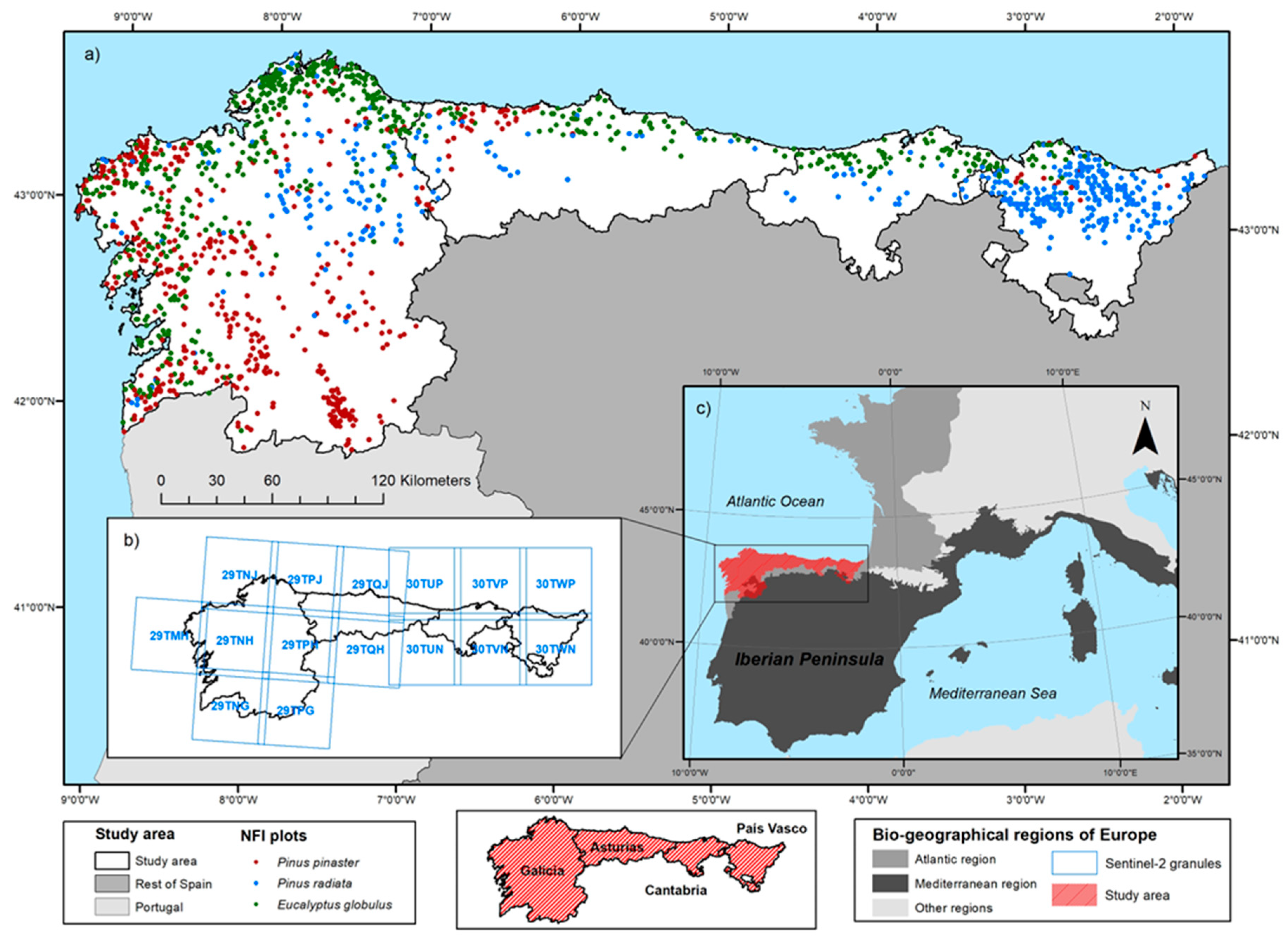
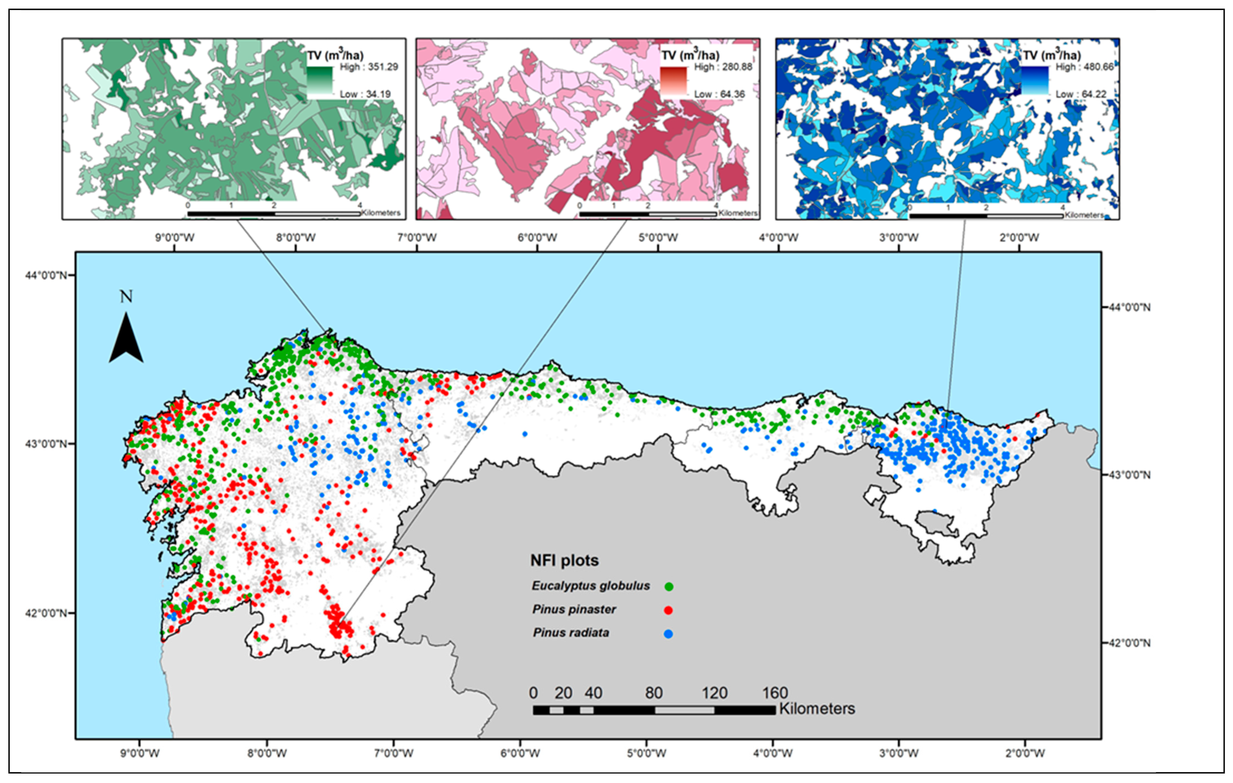
2.1. Study Area

This study was conducted in the four most productive forest regions in Spain (Galicia, Asturias, Cantabria and the Basque Country), which cover a total area of 52,821.44 km². Most of this area is included in the European Atlantic Bio-Geographical Region [29] (Figure 1), which is characterized by mild temperatures (mean annual temperatures varying between 11.5 °C and 14.5 °C) and precipitation that is quite uniformly distributed throughout the year and is often more than 1000 mm per year [30]. These favorable climatic conditions make this area very important for forestry in Spain. Forests occupy an area of 25,158 km² [31] in the study region, representing 47.6% of the total surface area. The landscape is complex, and the different combinations of topographic variables and landform strongly influence the type and vigor of the vegetation communities. Considering the area occupied, Eucalyptus globulus is the dominant forest species (22.5%), followed by Pinus pinaster (20.2%), Quercus robur (15.5%), Quercus pyrenaica (8%), Castanea sativa (8%), Pinus radiata (7.5%) and Fagus sylvatica (5.7%) [32].

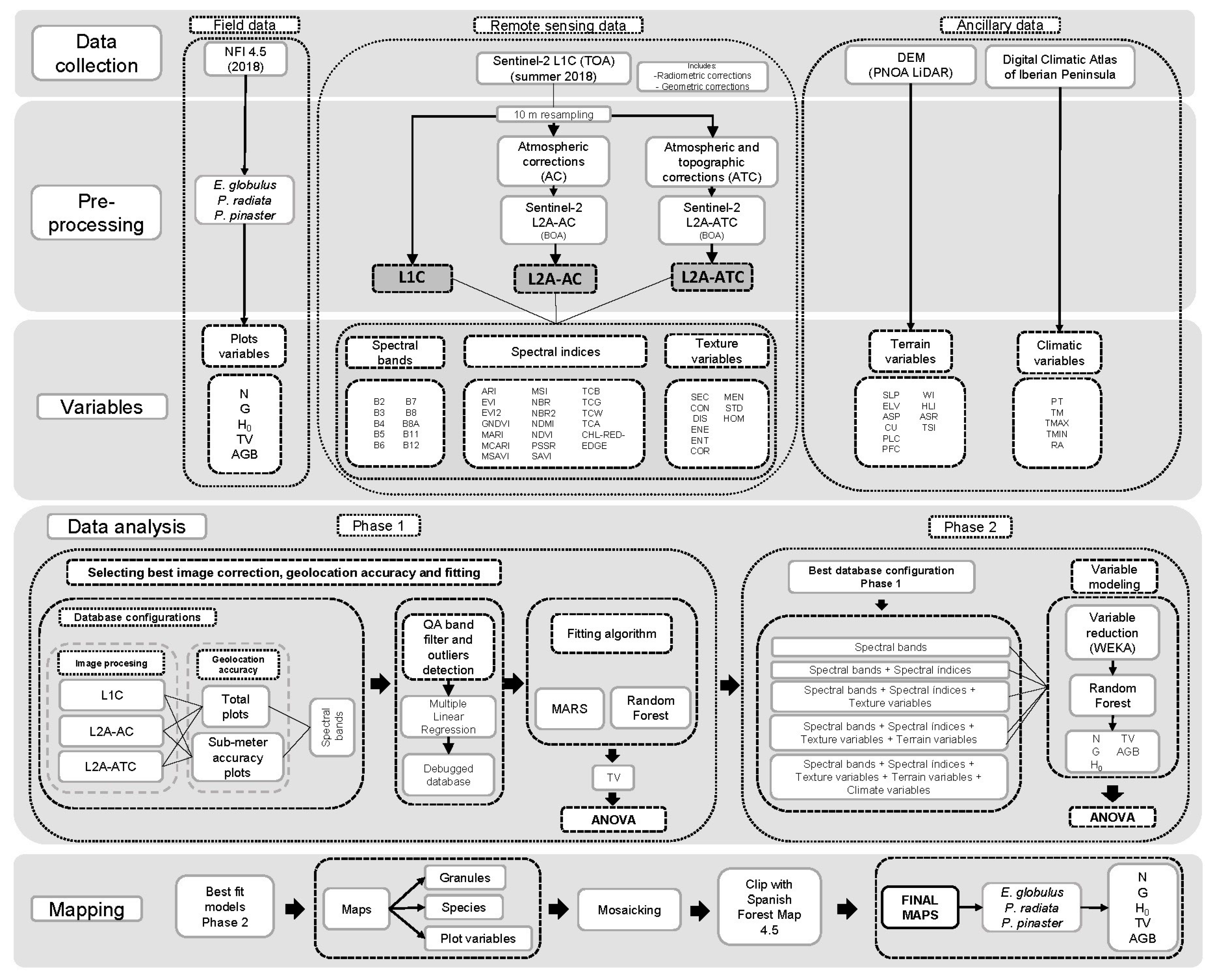
2.2. Data Collection and Pre-Processing

Four different types of data were used to develop the wall-to-wall remote sensed-based forest models: (i) field data; (ii) remotely sensed data; (iii) terrain data; and (iv) climatic data.

2.2.1. Field Data

The field plot data used in this study were obtained from the Spanish National Forest Inventory (SNFI) conducted by the Spanish Ministry of Agriculture, Fishing and Food [32]. The SNFI operates on a ten-year cycle, except for more productive forest species in northern Spain, for which a five-year cycle is used. We used the data from the last update of this inventory (SNFI 4.5), which was conducted in 2018 for the three most productive forest species in the study region: Tasmanian blue gum (E. globulus), maritime pine (P. pinaster) and radiata pine (P. radiata). In this inventory, the sampling plots are located at the intersections of a 1 × 1 km UTM grid comprising four concentric subplots of radius of 5, 10, 15 and 25 m, with a minimum diameter at 1.3 m aboveground level and thresholds of 75, 125, 225 and 425 mm, respectively [33].

Although the SNFI initially did not provide accurate coordinates, new remote sensing techniques have demonstrated the need for accurate coordinates [34] when using SNFI data to develop wall-to-wall forest models. The plot positioning of the fourth SNFI has an expected average theoretical accuracy of approximately 3–5 m [35], although the errors will actually be much greater in practice [14]. This led to the SNFI to capture new coordinates with errors less than 1 m in 73.36% of the plots in last remeasurement in 2018 (SNFI 4.5), making it easier to combine the field plot data with the information provided by remote sensing systems [36]. We therefore had available plots with low and high geolocation accuracy.

Plots of the three planted species of interest were established in pure stands (basal area 80% of the total basal area within the plot). Following this criterion, a total of 1471 plots within the study area were available for analysis. Among these plots, 589 were dominated by E. globulus, 474 by P. pinaster and 408 by P. radiata. Forest state variables such as the number of stems per hectare (N), basal area (G), dominant height (H₀), total over bark volume (TV) and aboveground biomass (AGB) were calculated from tree variable measurements and by using appropriate expansion factors. Stand-level species-specific allometric models developed for the same ecoregion by [37] were used to estimate aboveground biomass per plot.

Table 1. Descriptive statistics of the dependent variables analyzed in this study (number of stems per hectare, N; basal area, G; dominant height, H₀; total over bark volume, TV; and total aboveground biomass, AGB) extracted from the SNFI-4.5 plots where dominant species basal area was equal to or greater than 80% of the total basal area.

Species	No. Plots	Forest Variable	Descriptive Statistic
			Mean	Min.	Max.	Std.
E. globulus	589	N (stems ha−1)	833.83	10.19	2695.02	499.93
		G (m2 ha−1)	18.30	0.44	52.25	0.44
		H0 (m)	21.43	6.70	43.55	7.26
		TV (m3 ha−1)	148.42	0.68	522.67	118.14
		AGB (Mg ha−1)	99.44	0.98	371.55	81.68
P. pinaster	474	N (stems ha−1)	574.60	10.19	3176.03	439.15
		G (m2 ha−1)	22.60	0.42	55.73	13.70
		H0 (m)	16.67	3.40	31.78	6.34
		TV (m3 ha−1)	164.05	0.88	460.72	119.37
		AGB (Mg ha−1)	92.26	0.80	298.64	68.25
P. radiata	408	N (stems ha−1)	453.66	25.46	1773.48	294.07
		G (m2 ha−1)	27.82	0.67	66.62	13.54
		H0 (m)	22.55	5.70	39.55	6.28
		TV (m3 ha−1)	246.23	2.25	699.31	147.64
		AGB (Mg ha−1)	127.43	1.59	356.93	75.38

summarizes the descriptive statistics of the stand-related yield variables considered for the three forest species in the study area.

The distribution of the species under study and classification of vegetation types were determined using the Spanish Forest Map (Figure 1) (scale 1:25,000, minimum mapping unit of 1 ha), developed in coordination with SNFI-4.5.

2.2.2. Sentinel-2 Remote Sensing Data

We used freely available multispectral Sentinel-2 satellite (two twin-polar orbiting satellites) images, downloaded from the Copernicus Open Access Hub (https://dataspace.copernicus.eu/, accessed on 21 December 2023). These images were subjected to several corrections, and different spectral bands, indices and texture features were selected as independent remotely sensed variables for the present study (see Figure 2 for details of the workflow).

Image Pre-Processing Levels and Spectral Bands

Sentinel-2 data are available in different processed forms. The images we used were obtained in Level-1C product format (TOA, Top-Of-Atmosphere reflectance in cartographic geometry) in UTM/WGS84 projection and with less than 10% cloud cover. The Level-1C processing includes geometric corrections, radiometric processing and mask generation. After implementing atmospheric and topographic corrections with the Sen2Cor 2.8 tool [38], the Level-1C images were converted to Level-2A Bottom-Of-Atmosphere (BOA) reflectance images. To implement the corrections with Sen2Cor 2.8 tool, we used a digital elevation model (DEM) of 5 m of spatial resolution, developed in Spain by the National Center for Geographic Information (CNIG). The study area includes mountainous areas with sloping terrain, and topographic corrections of images may therefore play an important role. In this case, we used a bidirectional reflectance distribution function (BRDF) correction for vegetated mountainous with the recommended standard by ESA [39]. This correction is not available to download in the official ESA repository and must be generated by users. We therefore considered three pre-processing levels for the Sentinel images: (i) level L1C, scenes with geometric and radiometric corrections; (ii) level L2A-AC, scenes with geometric, radiometric and atmospheric corrections; and (iii) level L2A-ATC, scenes with geometric, radiometric, atmospheric and topographic corrections (for more information about Sentinel product types, see https://sentinels.copernicus.eu/web/sentinel/technical-guides/sentinel-2-msi/products-algorithms/, accessed on 21 December 2023, and [40]).

On the other hand, the Sentinel-2 Level-2A product enables masking different types of pixels at 20 and 60 m resolution by merging the information obtained from cirrus cloud detection and cloud shadow detection. For this study, we only used the pixels classified as vegetation (scene classification label = 4; more information available in https://sentinels.copernicus.eu/web/sentinel/technical-guides/sentinel-2-msi/level-2a/algorithm-overview/, accessed on 21 December 2023).

The satellite imagery was acquired between 14 June and 27 August 2018 (i.e., the same year that the field sampling was carried out), with fifteen tiles being necessary to cover the region of interest in northern Spain. A brief description of the images used is given in

Table 2. Acquisition dates and solar angles of fifteen Sentinel-2 scenes.

Satellite/Granule	Acquisition Date	Solar Zenith (°)	Solar Azimuth (°)
S2A/29TMH	11 August 2018	30.86	148.82
S2A/29TNG	19 June 2018	22.94	138.83
S2A/29TNH	11 August 2018	30.42	150.94
S2A/29TNJ	11 August 2018	31.22	151.58
S2A/29TPG	19 June 2018	22.36	141.25
S2B/29TPH	14 June 2018	23.10	143.23
S2B/29TPJ	24 June 2018	23.95	143.16
S2B/29TQH	24 June 2018	22.67	144.43
S2B/29TQJ	24 June 2018	23.41	145.61
S2A/30TUN	5 August 2018	29.46	146.64
S2A/30TUP	5 August 2018	30.25	147.34
S2A/30TVN	5 August 2018	29.00	148.81
S2A/30TVP	5 August 2018	29.80	149.51
S2B/30TWN	27 August 2018	35.52	153.22
S2B/30TWP	27 August 2018	36.34	153.70

.

All bands with 10 and 20 m spatial resolution were selected for inclusion in the classification procedure, but the spatial resolution of the 20 m bands was later increased to 10 m by using the nearest neighbor resampling method (

Table 3. Description of the ten Sentinel-2 bands used in this study.

Band	Symbol	Spectral Region	Wavelength (µm)	Spatial Resolution (m)
Band 2	B2	Blue	0.46–0.52	10
Band 3	B3	Green	0.54–0.58	10
Band 4	B4	Red	0.65–0.68	10
Band 5	B5	Red-Edge-1 (RE1)	0.70–0.71	20
Band 6	B6	Red-Edge-2 (RE2)	0.73–0.75	20
Band 7	B7	Red-Edge-3 (RE3)	0.76–0.78	20
Band 8	B8	Near-Infrared (NIR)	0.78–0.90	10
Band 8A	B8A	Narrow NIR (nNIR)	0.85–0.87	20
Band 11	B11	Shortwave infrared (SWIR-1)	1.56–1.65	20
Band 12	B12	Shortwave infrared (SWIR-2)	2.10–2.28	20

).

Spectral Indices

Spectral indices are simple numerical indicators that reduce multispectral (two or more spectral bands) data to a single variable for predicting and assessing vegetation characteristics, which is why they are also known as vegetation indices [41]. The high spectral resolution of Sentinel-2 imagery enables extraction of different indices from the spectral bands. Thus, 19 spectral indices were derived from the Sentinel-2 bands and the resultant quality scene classification band for each Sentinel-2 scene. These spectral indices are shown in

Table 4. Characteristics considered as candidate independent variables of the forest models.

Group	Variable Name
Spectral bands	Band 2—Blue (B2), Band 3—Green (B3), Band 4—Red (B4), Band 5—Vegetation Red-Edge-1 (B5), Band 6—Vegetation Red-Edge-2 (B6), Band 7—Vegetation Red-Edge-3 (B7), Band 8—NIR (B8), Band 8A—Narrow NIR (B8A), Band 11—SWIR-1 (B11), Band 12—SWIR-2 (B12).
Spectral indices	Anthocyanin Reflectance Index (ARI), Chlorophyll Red-Edge (CRE), Enhanced Vegetation Index (EVI), Enhanced Vegetation Index 2 (EVI2), Green Normalized Difference Vegetation Index (GNDVI), Modified Anthocyanin Reflectance Index (MARI), Modified Chlorophyll Absorption in Reflectance Index (MCARI), Modified Soil Adjusted Vegetation Index (MSAVI), Modified Soil Adjusted Vegetation Index (MSI), Normalized Burn Ratio (NBR), Normalized Burn Ratio 2 (NBR2), Normalized Difference Moisture Index (NDMI), Normalized Difference Vegetation Index (NDVI), Pigment-Specific Simple Ratio (PSSR), Soil Adjusted Vegetation Index (SAVI), Tasseled Cap Angle (TCA), Tasseled Cap Brightness (TCB), Tasseled Cap Greenness (TCG), Tasseled Cap Wetness (TCW).
Texture	Angular Second Moment (SEC), Contrast (CON), Correlation (COR), Dissimilarity (DIS), Energy (ENE), Entropy (ENT), Homogeneity (HOM), Max (MAX), Mean (MEN), Standard Deviation (STD).
Terrain	Aspect (ASP), Aspect/Slope Ratio (ASR), Curvature (CU), Elevation (ELV), Heat Load Index (HLI), Plan Curvature (PLC), Profile curvature (PFC), Slope (SLP), Terrain Shape Index (TSI), Wetness Index (WI).
Climatic	Average Temperature (TM), Maximum Temperature (TMAX), Minimum Temperature (TMIN), Precipitation (PT), Radiation (RA).

, and the formulation used can be consulted in Supplementary Material (Table S1).

Texture Variables

Textural variables are used to try to explain different relationships between object pixel and neighboring pixels, although the results are influenced by window size and directions [42]. If the window size is small, the differences within the kernel can often be exaggerated, increasing the noise content in the texture image. With a larger window size, the sample size increases, thus smoothing the textural variation and leading to relevant information about the texture being overlooked [43]. Different authors have tested different window sizes and directions (e.g., [42,44]). Window sizes of 7 × 7 or less and directions of 90 degrees have been found to be successful, as they enable the differences between the pixels occupied by trees and the ground to be captured while minimizing noise [45]. We used an optimized window size of a kernel 7 × 7 m to calculate 10 textural features derived from the derived from the Normalized Difference Vegetation Index (NDVI) using the Grey Level Co-occurrence Matrix (GLCM) texture extraction method [46] in the Sentinels Application Platform 9.0.0 (SNAP) software, which can be found at https://step.esa.int/main/download/snap-download/, accessed on 21 December 2023. The use of texture variables derived from spectral data has yielded satisfactory results in forest variables estimation (e.g., [44,47,48]).

Finally, as result of the Sentinel-2 image information extraction process, we recorded 39 layers (10 spectral bands + 19 spectral indices + 10 texture features) for each Sentinel-2 scene (Table 4). As previously commented, these 39 layers were available at three pre-processing levels: (i) level L1C (scenes with geometric and radiometric correction); (ii) level L2A-AC (scenes with geometric, radiometric and atmospheric corrections); and (iii) level L2A-ATC (scenes with geometric, radiometric, atmospheric and topographic corrections).

2.2.3. Ancillary Data

Two types of auxiliary variables were considered in this study: terrain and climatic variables.

Terrain Variables

To support the terrain analysis, a digital elevation model (DEM) of spatial resolution 5 m, developed by the Spanish National Center for Geographic Information (CNIG), was obtained. This model is available for free download at http://centrodedescargas.cnig.es/CentroDescargas/, accessed on 21 December 2023. We derived 10 terrain variables from the DEM of the CNIG as the average value of pixels inside each sample plot (see Table 4). This was resampled to 10 m/pixel resolution using the cubic convolution resampling method. Terrain variables are important and influence trees distribution, growth and yield [49], which is why we also included these variables with the aim of assessing their contribution for improving predictions of forest variables. The variables were generated using ArcGIS 10.8 software [50], which was selected on the basis of its wide use in previous studies (e.g., [18]).

Climatic Variables

Five climate variables were obtained for each pixel of 200 m spatial resolution (Table 4) from the Digital Climatic Atlas of the Iberian Peninsula [51]. This atlas is published on the internet at https://opengis.grumets.cat/wms/iberia/index.htm, accessed on 21 December 2023. The variables were resampled to 10 m/pixel using the nearest neighbor resampling method applied here. Solar radiation, temperature and precipitation variables drive plant growth and water availability in forest ecosystems. It is therefore reasonable to use the climatic features as independent variables when building the models. Moreover, within the framework of uncertain global climate change, production of different forest ecosystems may vary in the coming decades. The inclusion of climatic variables as independent variables in the models may enable comparison of different estimates obtained in the future.

2.3. Data Analysis, Model Fitting and Evaluation

2.3.1. Data Analysis

As the final result of the “Data collection and pre-processing” stage of this study, we had available a set of 54 variables (grouped in five groups) as candidate independent variables to be included in the models for predicting forest variables for three major commercial timber plantations in northern Spain. Data analysis was accomplished in two different phases (see Figure 2).

Analysis in Phase 1

This phase consisted of outlier analysis and subsequent selection of the best option from among the different levels of three qualitative factors: image correction, geolocation accuracy and algorithm fitting. The first step was the outlier detection caused by various factors, such as sensor errors, atmospheric interference, cloud cover, shadows, or land cover changes, and data debugging process, which consisted of the following sub-steps for each forest species: (i) applying the vegetation classification mask derived from Sentinel-2 Level-2A product; (ii) fitting a multilinear model to the dependent variable (TV) with the spectral bands as independent variables (10 variables); (iii) use of the stepwise regression method to eliminate the independent variables (of the 10 considered) that do not contribute to the model, (iv) fitting a multilinear model to the dependent variable (TV) with the remaining independent variables, and (v) plotting studentized residuals against leverage to detect outliers and/or observations with high leverage and extract these outliers to debug the database. To carry out this process, we used the R library, Tools for Building OLS Regression Models (olsrr) in R 4.0 statistical software (https://cran.r-project.org/, accessed on 21 December 2023). We used TV as a dependent variable in phase 1 of the analysis as it is usually the most important variable from the point of view of estimating forest resources.

After the data debugging process, a database was generated for each forest species (E. globulus, P. pinaster and P. radiata) considering three different levels of image processing (L1C, L2A-AC and L2A-ATC), two levels of plot geolocation accuracy (all plots and only sub-meter geolocation plots). This database was fitted to total over bark volume (TV) using two different algorithms, Random Forest (RF) and Multivariate Adaptive Regression Splines (MARS), with the spectral bands as independent variables. We used the total over bark volume (TV) as a dependent variable (it is currently the most important forest yield variable) with the sole aim of choosing the best alternative.

Separate one-way analysis of variance (ANOVA) was performed for the TV response variable, to test the effect of the different factors considered (image correction, plot geolocation accuracy and fitting algorithm), regardless of the species. Tukey’s honestly significant difference (HSD) multiple range test was used to determine homogeneous groups according to the similarity of the root mean square error (RMSE).

Analysis in Phase 2

After selecting the best image correction, geolocation accuracy and fitting techniques, we proceeded to the second phase of the data analysis (see Figure 2). This consisted of selecting five different groups of predictor variables in a cumulative process to determine the influence or importance of each group of variables in the final prediction. The following groups of predictor variables were considered:

• Spectral bands.
• Spectral bands + spectral indices.
• Spectral bands + spectral indices + texture variables.
• Spectral bands + spectral indices + texture variables + terrain variables.
• Spectral bands + spectral indices + texture variables + terrain variables + climatic variables.

We also performed ANOVA for each forest response variable (N, G, H₀, TV and AGB) and forest species, in order to test the contribution of each of the five different groups of predictors to the response variable. Tukey’s HSD multiple range test was used to determine homogeneous groups according to the similarity of the RMSE.

2.3.2. Modelling Techniques

In the past, quantitative predictions of most forest variables by means of remote sensing have involved traditional parametric regression techniques (e.g., [52,53,54]). However, this may not be suitable for analysis involving a potentially large number of predictors with complex interactions [55], as when dealing with remote sensing data. In the last few decades, the popularity of nonparametric methods has increased greatly for several reasons: (i) the speed and ease of implementation; (ii) the absence of restrictive assumptions; and (iii) the ability of some methods to include categorical dependent and (or) independent variables [54]. Among the numerous nonparametric techniques, we selected two widely used techniques for comparison: Random Forest and Multivariate Adaptive Regression Splines.

Random Forest (RF) regression techniques, first proposed by [56], are nonparametric techniques consisting of an ensemble of decision trees. This algorithm can be used for classification and regression and has been widely used in this type of research (e.g., [10,54,57,58,59]). In this technique, different independent variables, from the total set, are randomly selected to developed numerous decision trees. With randomized sampling, the accuracy and stability are improved relative to a single decision tree approach [60]. When RF is used in regression, the final value for each sample is given by the weighted average obtained from the estimates of individual trees [56]. The user can select the number of stems and the independent variables (predictors) used to configure the algorithm. This nonparametric approach is not greatly influenced by the number of input data or the multicollinearity of the data [61].

Multivariate Adaptive Regression Splines (MARS), a well-known nonparametric technique first proposed by [62], provides very good results for estimating forest variables from remote sensing data (e.g., [26,63,64]). MARS enables modelling a target variable based on multiple predictor variables using splines. A spline is a curve than can be fixed at different points or knots, where the relationship between the target variable and the independent variables changes. It thus generates piece-wise linear models in the distinct intervals of the predictor variables. MARS finds the end points of these intervals in two steps, by first overfitting the model with more knots than required and then removing the knots that contribute least to the overall model fit. Hence, regression splines are continuous smooth functions that fit the distribution of the data. However, MARS has various drawbacks: its functions tend to overfit with input data, and parameter choice is complicated and may require several iterations to find the best combination [55].

2.3.3. Model Assessment and Evaluation

Repeated 10-fold cross-validation was used to evaluate the models. The data are first split into k folds (groups) of the same size. One group is then selected as test data and the k-1 fold is used to adjust the model, and the goodness-of-fit statistics is calculated for this k-fold. This process was repeated k times using all k-folds as test folds. Finally, when the k-fold cross-validation was completed, we repeated the whole process 10 times, which is why it is named “repeated k-fold cross-validation”. Finally, the overall goodness-of-fit statistics were calculated as the average test statistics from 100 model runs (i.e., 10-fold cross-validation repeated 10 times using the training data).

The use of this validation technique is supported by various authors (e.g., [14,65]), although if the plot dataset is small, the use of this approach can have negative results [66].

Model performance was evaluated with several goodness-of-fit criteria, including the pseudocoefficient of determination (R²), the bias (Bias), the root mean square error (RMSE) and the relative values of these (Bias% and RMSE%).

The variable importance measure (VIM) was used to guide selection of predictors for the final models. To ensure that values of variable importance were expressed on comparable scales, the VIM values were normalized so that they summed to a unit value (normalized importance, VIM_N = (VIM − VIMmin)/(VIM_max − VIM_min)) and were also expressed in relative values (relative importance, VIM_R = VIM/∑VIM).

R statistical software [67] was used to implement the techniques compared in this study and to carry out Tukey’s HSD multiple comparison test.

2.4. Deriving Raster Maps

The models finally selected, for each species and forest state variable, were applied to the surface that each species occupies (areas greater or equal to 80%), according to the Spanish Forest Map 4.5, to generate spatially continuous maps with a spatial resolution of 10 m/pixel. Finally, applying the best algorithm, we obtained 15 maps, one for each of the five target variables of each species.

3. Results

As previously commented and shown in Figure 2, the results were obtained in two separate phases.

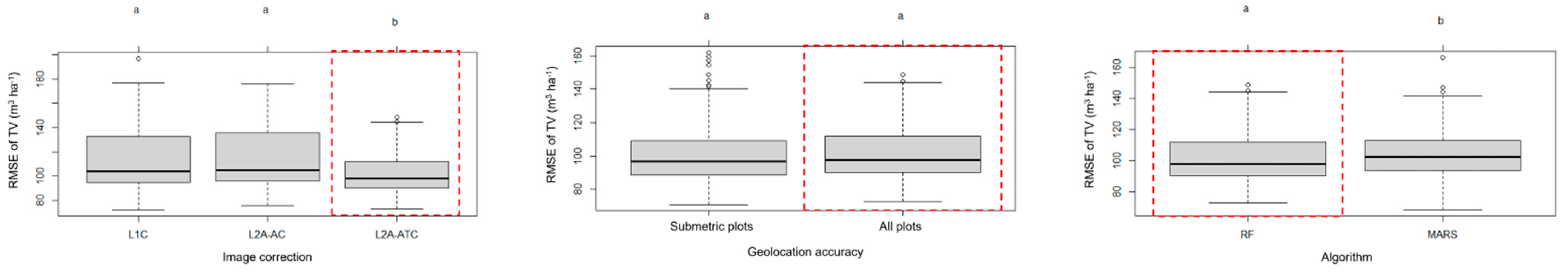
3.1. Phase 1: Best Data Configuration and Fitting Technique

Extraction of outliers to debug the database by applying the vegetation classification mask and using the plots of studentized residues against leverage enabled elimination of between approximately 5.88 and 13.29% of the plots for each configuration. The P. pinaster plots of the L1C level were the most refined, with removal of 13.29% as outliers, and the least refined were P. radiata plots of the L1C and L2A-AC level, with removal of 5.88% as outliers (

Table 5. Number of outliers for each dataset configuration.

Species	E. globulus			P. pinaster			P. radiata
Image Correction	L1C	L2A-AC	L2A-ATC	L1C	L2A-AC	L2A-ATC	L1C	L2A-AC	L2A-ATC
Total plots	589	589	589	474	474	474	408	408	408
Outliers	13 + 32	13 + 32	13 + 32	36 + 27	36 + 26	36 + 23	4 + 20	4 + 20	4 + 23
% Outliers	7.64	7.64	7.64	13.29	13.08	12.44	5.88	5.88	6.61

where outliers = plots removed from the application of vegetation classification mask + detection of influential observations from residuals vs. leverage plots.

).

According to the above criteria, from a total of 1471 plots within the study area, 1343 were finally available for analysis after applying the vegetation classification mask derived from Sentinel-2 Level-2A product and then removing influential observations from residuals vs. leverage plots (8.7%). Of these plots, 544 were dominated by E. globulus, 415 by P. pinaster and 384 by P. radiata.

After outlier detection and elimination, we had available for analysis a database of forest species which considered three different images processing levels, two different levels of plot geolocation accuracy and two model fitting algorithms. At this phase, as we were not building the final models, and to facilitate presentation of the results, we only used the most important yield variable, i.e., total over bark volume (TV), as a dependent variable to select the best alternative. These data configuration enabled (i) selection of the best image processing level, (ii) assessment of the effect of the quality of plot geolocation and (iii) selection of the best-fitting algorithm. The results of this process are shown in

Table 6. Summary of the goodness-of-fit statistics yielded by two regression algorithms (Multivariate Adaptive Regression Splines, (MARS) and Random Forest (RF)) for total over bark volume model (TV) and different image corrections and plot geolocation accuracy levels. All values represent the mean of 100 model runs (i.e., 10 replicates, each with 10-fold cross-validation).

Species	Image Correction	Geolocation Accuracy	No. Plot	MARS				RF
				R2	Bias	RMSE	RMSE%	R2	Bias	RMSE	RMSE%
E. globulus	L1C	All plots	544	0.36	−0.40	96.98	64.18%	0.35	−1.35	97.66	64.63%
		Sub-meter plots	457	0.34	−0.99	100.86	66.20%	0.34	−1.04	100.70	66.09%
	L2A-AC	All plots	544	0.33	0.72	98.43	65.61%	0.29	−0.91	100.73	67.15%
		Sub-meter plots	458	0.31	−0.07	102.37	67.91%	0.29	−0.75	103.50	68.66%
	L2A-ATC	All plots	544	0.37	0.19	94.53	63.69%	0.42	−0.89	90.76	61.15%
		Sub-meter plots	457	0.36	−0.32	97.49	65.45%	0.43	−0.59	91.11	61.17%
P. pinaster	L1C	All plots	411	0.37	−0.44	95.89	58.04%	0.33	−1.05	98.22	59.45%
		Sub-meter plots	351	0.38	−1.23	97.04	60.01%	0.37	1.10	97.09	60.03%
	L2A-AC	All plots	412	0.38	0.32	95.48	57.94%	0.36	−2.13	96.79	58.74%
		Sub-meter plots	353	0.39	0.40	96.24	59.55%	0.40	−2.28	94.84	58.69%
	L2A-ATC	All plots	415	0.32	−0.42	99.72	60.79%	0.38	−1.18	94.97	57.89%
		Sub-meter plots	354	0.37	0.22	98.04	60.78%	0.40	−1.29	94.55	58.62%
P. radiata	L1C	All plots	384	0.24	0.76	132.90	52.96%	0.12	−1.10	142.91	56.95%
		Sub-meter plots	172	0.24	−0.72	125.08	57.87%	0.09	−3.80	138.99	64.31%
	L2A-AC	All plots	384	0.27	0.21	132.02	52.61%	0.14	−2.60	145.22	57.87%
		Sub-meter plots	171	0.29	0.98	120.15	55.59%	0.11	−1.89	134.58	62.26%
	L2A-ATC	All plots	381	0.36	0.54	119.82	48.66%	0.36	0.37	118.45	48.10%
		Sub-meter plots	172	0.29	1.72	115.69	54.08%	0.26	−0.73	116.10	54.27%

where L1C = scenes with geometric and radiometric correction; L2A-AC = scenes with geometric, radiometric and atmospheric corrections; and L2A-ATC = scenes with geometric, radiometric, atmospheric and topographic corrections. All plots = all plots are used after elimination of outliers; Sub-meter plots = only plots with sub-meter geolocation are used.

.

Our findings indicate that the performance of the fitting algorithm depended on the image correction level adopted. Thus, MARS was the best-fitting technique for L1C and L2A-AC image corrections levels, whereas RF was the best approach for the L2A-ATC image correction level. Therefore, we must consider both characteristics together to select the best alternative. Thus, in almost all cases, geometrically, radiometrically, atmospherically and topographically corrected images (L2A-ATC) and RF algorithm provided the best fits. These results led us to select the L2A-ATC image correction level and the RF algorithm to be considered in phase 2 of the analysis. This was true for all goodness-of-fit statistics, except for bias in two of the three results obtained for the different species (Table 6). We decided to select RF for further analysis in phase 2, although the bias values obtained must be considered with caution, as it is highly recommended that final model be unbiased or with the lowest possible bias. In fact, Tukey’s HSD multiple comparison test produced significantly better results for the L2A-ATC correction level and the RF algorithm regardless of the species (Figure 3).

As we had available a proportion of plots where precise geolocation was guaranteed (sub-meter), we used two different databases to check the geolocation accuracy of the results: all plots and only plots with sub-meter geolocation. The goodness-of-fit statistics were used to compare both alternatives and the results obtained using the relative root mean square error for comparison purposes and considering the different image correction levels and the two algorithms used showed that the results for all the plots were higher (Table 6). In addition, Tukey’s HSD multiple comparison test yielded very similar results (not significantly different) for the two levels of geolocation accuracy (Figure 3). Based on these findings we decided to use the total number of plots to generate the final models in phase 2 of this study.

Average increases in the relative root mean square error values ranged from 1.56% to 8.50% for comparison of the total over bark volume (TV) estimates for L2A-ATC correction with L1C-corrected images. The greatest improvement (8.50%) corresponded to P. radiata, stands of which generally grew on the steepest slope (average, 35.93%). By contrast, the lowest increment (1.56%) corresponded to P. pinaster, stands of which grew on less steep terrain (average slope, 23.76%) (

Table 7. Relative root mean square error values yielded by the RF algorithm (see Table 8) for species and considering the average slope and aspect of the plots. Values within brackets indicate the percentage gain in RMSE relative to the L1C values.

Species		E. globulus	P. pinaster	P. radiata
Image correction	L1C	64.63%	59.45%	56.95%
	L2A-AC	67.15% (−2.51%)	58.74% (+0.72%)	57.87 (−0.92%)
	L2A-ATC	61.15% (+3.49%)	57.89% (+1.56%)	48.10 (+8.50%)
Plot variable	Average slope (%)	28.06	23.76	35.93
	Average aspect (°)	179.14	179.21	179.60
	% Plots with slope > 20%	67.91	52.95	75.74

).

3.2. Phase 2: Contribution of Each Group of Predictor Variables and Final Fitting Models

3.2.1. Contribution of Each Group of Predictor Variables

Analysis of the contribution of each of the five groups of predictor variables revealed differences according to the species. Thus, considering the results in

Table 8. Comparison of the RF regression models for forest variables by species. Column (1) includes the value of the goodness-of-fit statistics using only spectral bands as predictors. The other columns show the percentage of change in the value of the statistics when using more predictor variables compared to (1). All values represent the mean of 100 model runs (i.e., 10 replicates, each with 10-fold cross-validation). The values highlighted in bold correspond to the data group selected as the best option for each combination of dependent variable and species.

Type	Dependent Variable	Statistic	Eucalyptus globulus					Pinus pinaster					Pinus radiata
			Group of Predictor Variables					Group of Predictor Variables					Group of Predictor Variables
			(1)	(2)	(3)	(4)	(5)	(1)	(2)	(3)	(4)	(5)	(1)	(2)	(3)	(4)	(5)
Density	Number of stems, N (stems ha−1)	R2	0.24	+4.17%	+8.33%	+8.33%	+8.33%	0.15	+6.67%	+26.67%	+40.00%	+53.33%	0.1	+20.00%	+60.00%	+80.00%	+50.00%
		Bias	4.64	+34.91%	+65.52%	+17.24%	+62.72%	−4.91	+61.30%	+102.85%	+92.26%	+178.00%	−6.02	−9.30%	+20.43%	+13.79%	+33.06%
		RMSE	438.49	-0.88%	−1.34%	−1.48%	−1.20%	412.04	−2.70%	−4.18%	−5.30%	−6.63%	283.12	−1.60%	−3.78%	−5.09%	−3.87%
	Basal área, G (m2 ha−1)	R2	0.40	+10.00%	+12.50%	+15.00%	+15.00%	0.41	0.00%	+12.20%	+12.20%	+12.20%	0.33	0.00%	+9.09%	+18.18%	+18.18%
		Bias	−0.05	−20.00%	+20.00%	+40.00%	+80.00%	−0.08	−25.00%	−50.00%	−50.00%	+25.00%	−0.01	−300.00%	−500.00%	+100.00%	−500.00%
		RMSE	9.50	−3.26%	−3.68%	−4.63%	−4.42%	10.59	+0.38%	−4.53%	−4.25%	−4.72%	11.18	0.00%	−2.15%	−5.10%	−5.10%
Size	Dominant height, H0 (m)	R2	0.26	+3.85%	+11.54%	+23.08%	+26.92%	0.26	+7.69%	+7.69%	+34.62%	+42.31%	0.28	+14.29%	+21.43%	+32.14%	+28.57%
		Bias	0.04	−75.00%	−100.00%	−200.00%	−150.00%	−0.04	+50.00%	+50.00%	+100.00%	+25.00%	−0.01	+300.00%	−300.00%	−400.00%	−500.00%
		RMSE	6.31	−0.63%	−2.06%	−4.28%	−4.75%	5.49	−1.28%	−1.28%	−6.38%	−7.47%	5.36	−2.61%	−4.66%	−6.16%	−5.97%
Yield	Total volume with bark, TV (m3 ha−1)	R2	0.41	+7.32%	+9.76%	+12.20%	+12.20%	0.38	+2.63%	+7.89%	+10.53%	+18.42%	0.37	+2.70%	+8.11%	+18.92%	+16.22%
		Bias	−0.62	+24.19%	+122.58%	+35.48%	+35.48%	−1.15	−45.22%	+20.00%	+37.39%	−11.30%	0.11	+254.55%	+618.18%	−27.27%	+218.18%
		RMSE	91.21	−3.03%	−3.66%	−4.14%	−4.14%	94.53	−1.03%	−2.84%	−3.09%	−5.11%	117.94	−1.09%	−2.42%	−5.27%	−4.58%
	Aboveground Biomass, AGB (Mg ha−1)(Mg/ha)	R2	0.41	+4.88%	+2.44%	+4.88%	+4.88%	0.36	+2.78%	+8.33%	+11.11%	+13.89%	0.35	+5.71%	+8.57%	+20.00%	+20.00%
		Bias	−0.79	+16.46%	+40.51%	+31.65%	+20.25%	−1.03	+2.91%	−27.18%	−35.92%	−35.92%	−0.41	−82.93%	−168.29%	−119.51%	−48.78%
		RMSE	63.13	−2.47%	−1.39%	−2.14%	−2.08%	54.88	−0.80%	−2.53%	−3.37%	−3.81%	61.15	−1.77%	−2.29%	−5.10%	−4.73%

where R² = pseudocoefficient of determination, Bias = bias, RMSE = root mean square error. (1) = spectral bands; (2) = spectral bands + spectral indices; (3) = spectral bands + spectral indices + texture variables; (4) = spectral bands + spectral indices + texture variables + terrain variables; (5) = spectral bands + spectral indices + texture variables + terrain variables + climatic variables.

and the averaged results of the five forest models for each species shows that the contribution of spectral bands only (dataset 1) is higher for E. globulus (R² = 0.34) and decreases for P. pinaster (R² = 0.31) and P. radiata (R² = 0.29). Since the average performance of the final models for different species is quite similar, this implies a greater contribution of the other predictor variables for P. pinaster and P. radiata. Thus, for eucalypt, there is only an average increase in R² (considering the five dependent variables) of 13.47% for models fitted with the best dataset relative to dataset 1, whereas this increased to 28.03% and 26.59%, for maritime pine and radiata pine, respectively. For E. globulus, we observed a moderate-high contribution of spectral indices (group 1) and low contribution of textural (group 3) and terrain variables (group 4). Although textural and terrain variables make a large contribution for radiata pine and maritime pine, structural indices make a large contribution for radiata pine and a low contribution for maritime pine (Table 8).

The climatic variables (group 5) did not make valuable contributions to the eucalypt and radiata pine models. However, this group of variables improved the models for maritime pine. Looking closely at the P. radiata results, the contribution of climatic variables is null or negative as they reduce the predictive ability of the models (see Table 8). For this species, the group 4 variables contribute to the best forest variables prediction including the spectral bands, spectral indices, texture and terrain variables. Climatic variables improve the models for P. pinaster, increasing the pseudocoefficient of determination up to 13.33% (6.34% on average) relative to the results obtained from the group of variables no. 4 (without climatic variables). This contribution was only negligible for the basal area model (Table 8). Although these are important improvements, according to Tukey’s HSD multiple comparison test (with the RMSE), many are not statistically significant. In fact, none of the improvements in groups of variables relative to the immediately adjacent group were statistically significant (Figure S2).

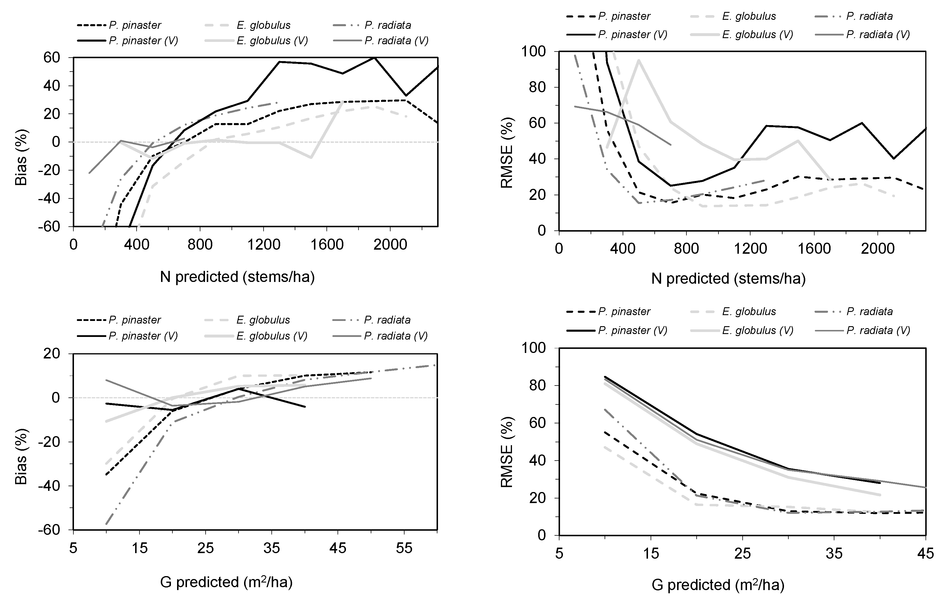
3.2.2. Model Prediction

Five forest variables were predicted from Sentinel-2-derived predictors and other ancillary variables. We considered two density variables (number of stems per hectare and basal area), one size-related variable (dominant height) and two yield variables (total over bark volume and total aboveground biomass). The models that produced the worst results were the number of stems per hectare (N), with R² ranging from 0.18 to 0.26 (relative RMSE ranged from 51.8% to 67.0%), followed by dominant height (H₀), with R² ranging from 0.33 to 0.37 (relative RMSE ranged from 22.3% to 30.5%). Yield variables, total over bark volume (TV) and aboveground biomass (AGB) and basal area (G) produced the best-fitting results, with R² greater than 0.40 (except G, for P. radiata, with R² = 0.39) and reaching up to 0.46 (

Table 9. Summary of the contribution of each group of independent variables to the predictive ability of models and their goodness-of-fit statistics. All values represent the mean of 100 model runs (i.e., 10 replicates, each with 10-fold cross-validation). The numbers in brackets represent the number of variables included in the model, and the number outside brackets indicate the accumulated importance measure expressed in relative values (VIM_R), where Avg. = average, VIM_R value of the five models, R² = pseudocoefficient of determination, Bias = bias, Bias% = relative bias, RMSE = root mean square error, RMSE% = relative root mean square error of the best models.

			Eucalyptus globulus						Pinus pinaster						Pinus radiata
			N	G	H0	TV	AGB	Avg.	N	G	H0	TV	AGB	Avg.	N	G	H0	TV	AGB	Avg.
Independent variables	Group	(1)	0.24 (2)	0.47 (4)	0.18 (2)	0.26 (2)	0.48 (6)	0.33	0.29 (2)	0.53 (3)	0.25 (3)	0.51 (4)	0.43 (3)	0.40	0.41 (5)	0.35 (4)	0.32 (4)	0.44 (4)	0.39 (3)	0.38
		(2)	0.55 (6)	0.36 (5)	0.47 (9)	0.56 (6)	0.52 (4)	0.50	0.34 (5)	0.20 (2)	0.23 (5)	0.13 (2)	0.23 (3)	0.23	0.28 (3)	0.31 (3)	0.29 (4)	0.24 (3)	0.22 (3)	0.26
		(3)	0.07 (1)	0.11 (2)	0.07 (2)	0.06 (1)	-	0.06	0.09 (3)	0.27 (3)	0.15 (3)	0.14 (2)	0.16 (2)	0.16	0.14 (1)	0.16 (3)	0.16 (3)	0.10 (2)	0.13 (4)	0.13
		(4)	0.14 (2)	0.06 (1)	0.17 (4)	0.13 (2)	-	0.10	0.20 (3)	-	0.23 (3)	0.07 (1)	0.08 (1)	0.12	0.17 (2)	0.17 (3)	0.23 (4)	0.22 (4)	0.27 (5)	0.21
		(5)	-	-	0.11 (3)	-	-	0.02	0.08 (1)	-	0.15 (2)	0.16 (2)	0.10 (1)	0.10	-	-	-	-	-	0.00
	No. of variables		11	12	20	11	10		14	8	16	11	10		11	13	15	13	15
Goodness-of-fit statistics		R2	0.26	0.46	0.33	0.46	0.43		0.23	0.46	0.37	0.45	0.41		0.18	0.39	0.37	0.44	0.42
		Bias	−5.44	−0.07	−0.02	−0.84	−0.92		−13.65	−0.10	−0.05	−1.02	−0.66		−6.85	−0.02	0.03	0.08	0.08
		Bias%	−0.007	−0.004	−0.001	−0.006	−0.009		−0.024	−0.005	−0.003	−0.006	−0.007		−0.015	−0.001	0.001	0.000	0.001
		RMSE	432.63	9.06	6.01	87.43	61.57		384.72	10.01	5.08	89.7	52.79		268.7	10.61	5.03	111.73	58.03
		RMSE%	51.8	49.5	28.0	58.9	61.9		67.0%	44.6	30.5	54.7	57.2		59.2	38.1	22.3	45.4	45.5

) (RMSE% ranged from 44.6% to 61.9%). However, all models displayed very low bias, with higher values for N models (values of Bias% ranged between −0.024% and 0.001%) (Table 9; Figure S1). Therefore, the models can be considered unbiased as the Bias% was always lower than 1% (average value of −0.006%).

Figure 4 shows the typical overall RMSE% increase for the validation dataset and the reduction in the Bias% as a consequence of the 100 iterations. These graphs show the model performance for classes of the predicted variable; all models (regardless of the response variable) performed similarly, overestimating lower values and underestimating higher values, although to a much lesser extent.

According to the VIM_R scores shown in Table 9, spectral bands contributed most to the P. pinaster and P. radiata models (averaged accumulated VIM_R of 40% and 38%, respectively), followed by the spectral indices (averaged accumulated VIM_R of 23% and 26%, respectively), with texture and terrain variables contributing 16% and 12% in P. pinaster and 13% and 22% in P. radiata. Climatic variables contributed the remaining 10% in P. pinaster and 0% in P. radiata (Table 9). However, important differences were observed according to the spectral variables with the highest VIM_R score; thus, the spectral bands that contributed most to the P. pinaster models were the short-wave infrared bands B11 and B12, representing 71% of the total contribution of this group of variables to the set of models, followed by red band (B4) and Red-Edge-1 (B5). By contrast, the green band (B3) and red band (B4) contributed most to the set of models in P. radiata, representing 43% of the contribution of this group of variables, followed by near-Infrared (B8) and short-wave infrared B11 (

Table 10. Variables included in the models and their relative variable importance values (VIM_R). Sum = sum of the VIM_R values of the five models.

Type	Indep. Variable	Eucalyptus globulus						Pinus pinaster						Pinus radiata
		N	G	H0	TV	AGB	Sum.	N	G	H0	TV	AGB	Sum.	N	G	H0	TV	AGB	Sum.
Spectral bands	B2	-	-	-	-	0.06	0.06	-	-	-	-	-	-	0.09	0.06	-	-	-	0.15
	B3	-	-	-	-	-	-	-	-	-	-	-	-	0.07	0.09	-	0.10	0.16	0.42
	B4	-	-	-	-	-	-	-	-	0.11	0.08	-	0.19	0.07	0.08	0.06	0.10	0.09	0.40
	B5	0.11	-	0.08	-	0.10	0.29	-	-	0.08	0.09	-	0.17	-	-	0.12	-	-	0.12
	B6	0.13	0.11	-	-	0.06	0.30	-	0.07	-	-	0.04	0.11	-	-	0.08	-	-	0.08
	B7	-	0.05	-	0.06	0.04	0.15	-	-	-	-	-	-	-	-	-	-	-	-
	B8	-	-	-	-	-	-	-	0.07	-	-	-	0.07	-	0.12	-	0.10	0.14	0.36
	B8A	-	0.06	-	-	0.04	0.10	-	-	-	-	0.04	0.04	-	-	0.06	-	-	0.06
	B11	-	0.26	0.10	0.20	0.19	0.75	0.20	0.39	0.06	0.19	0.34	1.18	0.11	-	-	0.14	-	0.25
	B12	-	-	-	-	-	-	0.08	-	-	0.14	-	0.22	0.07	-	-	-	-	0.07
Spectral indices	ARI	0.10	0.10	0.06	0.11	0.08	0.45	-	-	-	-	-	-	0.15	-	-	-	-	0.15
	CRE	-	-	-	-	-	-	-	-	-	-	-	-	0.06	-	-	-	-	0.06
	EVI	-	0.08	0.05	0.09	0.08	0.30	0.06	0.10	-	-	-	0.16	-	0.08	0.10	0.11	0.13	0.42
	EVI2	-	-	-	-	0.04	0.04	-	-	-	-	-	-	-	-	-	-	-	-
	GNDVI	-	0.06	-	-	-	0.06	0.08	-	0.04	0.06	-	0.18	-	0.06	0.05	0.05	0.05	0.21
	MARI	-	-	-	-	0.05	0.05	-	0.10	0.04	0.07	0.10	0.31	-	-	-	-	-	-
	MCARI	-	-	0.05	0.07	0.06	0.18	-	-	-	-	-	-	-	-	-	-	-	-
	MSAVI	-	0.07	-	0.06	-	0.13	-	-	-	-	0.05	0.05	-	-	-	-	0.04	0.04
	MSI	0.08	-	-	-	-	0.08	0.05	-	-	-	-	0.05	-	-	0.04	-	-	0.04
	NBR	-	-	-	-	-	0.07	-	-	0.05	-	-	0.05	-	-	-	-	-	-
	NBR2	-	-	0.03	-	-	0.03	0.10	-	0.04	-	-	0.14	0.06	-	-	-	-	0.06
	NDMI	-	-	0.08	-	-	0.08	0.05	-	0.06	-	-	0.11	-	-	-	-	-	-
	NDVI	-	-	-	-	-	-	-	-	-	-	-	-	-	-	-	-	-	-
	PSSR	0.08	-	0.03	-	-	0.11	-	-	-	-	-	-	-	-	-	-	-	-
	SAVI	-	-	-	-	-	-	-	-	-	-	-	-	-	-	-	-	-	-
	TCA	0.07	0.06	0.04	-	-	0.17	-	-	-	-	-	-	-	-	-	-	-	-
	TCB	0.14	-	0.07	-	-	0.21	-	-	-	-	0.08	0.08	-	0.17	-	-	-	0.17
	TCG	-	-	0.06	0.06	0.05	0.17	-	-	-	-	-	-	-	-	-	0.07	-	0.07
	TCW	-	-	0.09	0.17	0.16	0.42	-	-	-	-	-	-	-	-	0.09	-	-	0.09
Texture	SEC	-	-	-	-	-	-	-	-	-	-	-	-	-	-	-	-	0.03	0.03
	CON	-	-	-	-	-	-	-	-	-	-	-	-	-	-	0.05	-	0.04	0.09
	COR	-	0.05	-	-	-	0.05	-	-	-	-	-	-	0.14	0.06	-	-	-	0.20
	DIS	-	-	-	-	-	-	0.03	0.08	-	-	-	0.11	-	-	0.05	0.06	0.03	0.14
	ENE	-	-	-	-	-	-	0.03	-	-	-	-	0.03	-	0.05	-	0.04	-	0.09
	ENT	-	-	-	-	-	-	0.03	-	0.04	-	-	0.07	-	-	-	-	-	-
	HOM	0.07	-	-	-	-	0.07	-	-	0.04	-	-	0.04	-	0.05	-	-	0.02	0.07
	MAX	-	-	-	-	-	-	-	-	-	-	-	-	-	-	-	-	-	-
	MEN	-	0.06	0.04	0.06	-	0.16	-	0.10	0.06	0.07	0.09	0.32	-	-	-	-	-	-
	SDT	-	-	0.04	-	-	0.04	-	0.09	-	0.07	0.08	0.24	-	-	0.05	-	-	0.05
Terrain	ASP	-	0.06	0.04	0.06	-	0.16	-	-	-	-	-	-	-	0.07	0.05	0.06	0.06	0.24
	ASR					-	-	-	-	-	-	-	-	-	-	-	-	-	-
	CU	-	-	-	-	-	-	-	-	-	-	-	-	-	-	0.06	-	-	0.06
	ELV	-	-	0.04	-	-	0.04	-	-	0.14	0.07	-	0.21	-	-	-	0.05	0.06	0.11
	HLI	0.07	-	-	0.07	-	0.14	-	-	-	-	-	-	-	-	-	-	-	-
	PLC	0.07	-	-	-	-	0.07	0.06	-	-	-	0.08	0.14	-	0.05	-	-	-	0.05
	PFC	-	-	-	-	-	-	-	-	-	-	-	-	-	-	-	-	0.04	0.04
	SLP	-	-	0.04	-	-	0.04	0.06	-	0.04	-	-	0.10	0.08	-	0.07	0.05	0.05	0.25
	TSI	-	-	0.04	-	-	0.04	-	-	-	-	-	-	-	-	0.05	-	-	0.05
	WI	-	-	-	-	-	-	0.08	-	0.05	-	-	0.13	0.09	0.06	-	0.06	0.06	0.27
Climatic	TM	-	-	0.04	-	-	0.04	-	-	-	0.09	-	0.09	-	-	-	-	-	-
	TMAX	-	-	0.04	-	-	0.04	0.08	-	0.06	0.07	0.10	0.31	-	-	-	-	-	-
	TMIN	-	-	-	-	-	-	-	-	-	-	-	-	-	-	-	-	-	-
	PT	-	-	0.03	-	-	0.03	-	-	0.09	-	-	0.09	-	-	-	-	-	-
	RA	-	-	-	-	-	-	-	-	-	-	-	-	-	-	-	-	-	-

). The spectral indices that contributed most to P. radiata models were EVI, GNDVI, TCB and ARI, with an accumulated VIM_R of 0.95, which represented 73% of the contribution of this group of variables. For P. pinaster, the corresponding indices were MARI, GNDVI, EVI and NBR2, with an accumulated VIM_R of 0.79 which represents 70% of the contribution of this group of variables. The NDVI texture indices that contribute most to the models were CON, DIS, ENE and COR for P. radiata and MEN, SDT, ENT and DIS for P. pinaster, with accumulated VIM_R of 0.52 and 0.74, which represent contributions of 78% and 91%, respectively. The terrain variables that contributed most to the forest models were WI, SLP, ASP and ELV for P. radiata and ELV, WI, PLC and SLP for P. pinaster, with accumulated VIM_R of 0.87 and 0.58, which represent contributions of 81% and 100%, respectively. Climatic variables did not contribute to the P. radiata models, but did contribute to the P. pinaster models. Thus, only MAT contributed, with an accumulated VIM_R of 0.31, which represents a contribution of 63%.

For E. globulus, spectral indices contributed most to the forest models (averaged accumulated VIM_R = 0.50), with ARI, TCW, EVI and TCB contributing with an accumulated VIM_R of 1.38, which represented 55% of the total importance of this group of variables (Table 9). The following most important group of variables was the spectral bands (averaged accumulated VIM_R = 0.33). The four most relevant were B11, B6, B5 and B7, which contributed an accumulated VIM_R of 1.48, representing 90% of the importance of this group of variables. Terrain variables (averaged accumulated VIM_R = 0.10) were the third most important group of variables according to the averaged accumulated VIM_R score, with ASP, HLI, PLC and ELV representing 55.49% of the total importance of this group of variables. Texture was fourth group according to its contribution to ability prediction of eucalypt forest models, with an averaged accumulated VIM_R = 0.06. The variables MEN, HOM, COR and SDT contributed with an accumulated VIM_R of 0.41 (100% of the total importance of this group). Finally, climate made a very small contribution, with an averaged accumulated VIM_R = 0.02.

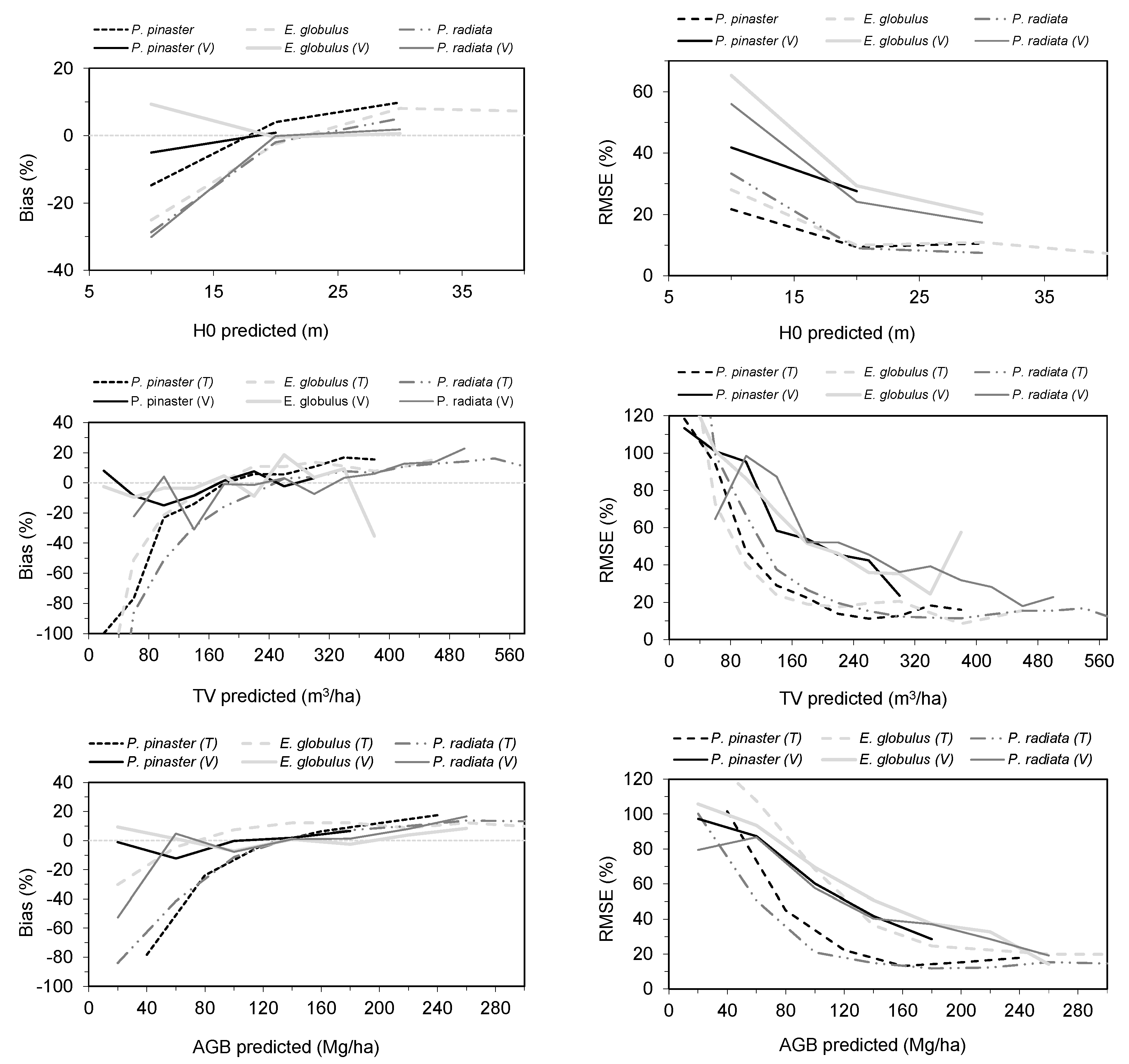
3.3. Results of Mapping Forest Variables

Spatially continuous maps of the forest variables resulting from application of the best models for the three major commercial timber plantations (E. globulus, P. pinaster and P. radiata), occupying areas greater or equal to 80% (according to the Spanish Forest Map) were generated. Figure 5 shows, as an example, the distribution of TV (m³ ha⁻¹) for the different forest species across the study area. Finally, average values per hectare and total Sentinel-2-based wall-to-wall predictions for the five forest variables and for the three species were generated per region (

Table 11. Table showing the average and standard deviation values per hectare and total of the Sentinel-2-based wall-to-wall predictions for the three forest species and the four regions in northern Spain.

		Region
		Galicia		Asturias		Cantabria		Basque Country
		Avg. (Sd)	Total	Avg. (Sd)	Total	Avg. (Sd)	Total	Avg. (Sd)	Total
E. globulus	N	816.42 (120.11)	108,162,865.38	782.00 (131.34)	30,174,276.15	790.58 (129.26)	26,771,979.95	868.86 (180.21)	8,625,895.65
	G	18.21 (3.95)	2,412,527.76	15.79 (3.34)	609,186.45	16.89 (4.07)	572,048.59	20.12 (6.37)	199,773.22
	H0	21.66 (2.03)	2,870,200.23	20.17 (1.49)	778,171.45	21.25 (1.88)	719,627.29	22.23 (2.81)	220,672.33
	TV	152.15 (38.17)	20,157,482.01	126.57 (29.66)	4,883,988.79	141.38 (38.21)	4,787,726.89	170.94 (61.01)	1,697,084.24
	AGB	103.48 (26.00)	13,709,146.49	86.45 (19.72)	3,335,870.38	95.80 (25.94)	3,244,040.50	117.41 (41.94)	1,165,589.52
P. pinaster	N	663.05 (129.72)	111,420.57	605.84 (92.03)	8,788,913,94	809.37 (271.92)	173,420.57	794.72 (185.78)	4,177,647.49
	G	21.19 (4.86)	3,569,806.40	22.90 (4.05)	322,160.32	25.96 (9.04)	5,561.59	27.65 (5.65)	145,354.34
	H0	15.88 (2.54)	2,675,987.48	15.95 (1.62)	231,398.86	16.19 (2.66)	3,468.13	17.69 (1.57)	92,982.27
	TV	156.43 (41.86)	26,353,790.70	164.17 (32.25)	2,381,631.85	197.49 (78.15)	42,316.14	208.83 (43.58)	1,097,773.53
	AGB	87.27 (24.04)	14,701,927.30	113.07 (26.48)	1,640,230.48	66.97 (16.88)	14,349.93	103.61 (26.08)	544,669.58
P. radiata	N	513.70 (87.71)	30,609,531.69	521.11 (76.32)	9,831,803.62	466.87 (76.92)	3,032,877.78	476.96 (64.09)	54,692,959.82
	G	26.05 (4.10)	1,552,099.38	26.99 (4.23)	509,313.68	26.32 (4.93)	171,007.17	27.80 (5.46)	3,187,960.25
	H0	20.52 (1.47)	1,222,504.17	20.44 (1.83)	385,672.55	21.70 (2.17)	140,998.67	23.24 (2.18)	2,664,458.16
	TV	215.59 (38.68)	12,846,469.77	222.08 (41.58)	4,189,903.77	230.08 (50.87)	1,494,652.27	259.30 (61.23)	29,733,439.08
	AGB	114.94 (20.58)	6,848,897.27	116.21 (21.72)	2,192,591.69	114.32 (27.88)	742,616.38	132.73 (30.24)	15,219,668.09

where Avg. = mean value of the forest variable (units of the variable per hectare); Sd = standard deviation of variables; Total = total amount of the variable (units of the variable); N = number of stems, G = basal area (m²), H₀ = dominant height (m), TV = total over bark volume (m³) and AGB = aboveground biomass (Mg).

).

4. Discussion

4.1. Impacts of Geolocation Accuracy, Image Correction Level and Fitting Algorithm on Total Volume Estimation

The study findings did not show any clear impact of the plot geolocation accuracy on the stand volumes estimated using Sentinel-2 data. Thus, contrary to what might be expected, the result of using all plots was better than the result of using only sub-meter plot accuracy. This seems to suggest that the model performance mainly depends on other characteristics of the plots used for the model development (e.g., stand age, density, …) rather than on the precision of the geolocation.

While is true that accurate geographical co-registration of remote sensing data and field plots has been recognized as necessary [24,68], its impact strongly depends on the size of the field plot and on the type of the remote sensor used (active or passive) and its spatial resolution.

Thus, ref. [24] showed that larger plot sizes (300–400 m²) compensate for errors; these results were later confirmed and extended by [69], who found that prediction improved markedly as plot size increased from 314 m² (10 m radius) to 1964 m² (25 m radius), the maximum size of the SNFI plots. In our study, 83.33% of the plots were of radius equal or greater than 15 m (52.08% have a radius of 25 m). There are two main reasons underlying these results [69]: (i) large plots capture more on-ground variability and therefore are more resistant to the harmful effects of co-registration errors and (ii) large plots maintain a greater amount of spatial overlap between land plot and LiDAR data. This latter was demonstrated by [35], who showed that for plot size of 1964 m² (25 m radius) and positioning errors of 5 and 10 m (much larger than the 3–5 m theoretical errors), the areas overlapping a plot in a correct position and a plot located in an altered position were 84.3% and 74.7%, respectively. These previous arguments, which mainly concern LiDAR actively remotely sensed data, are also applicable to passively remotely sensed data. Ref. [70] found than co-registration errors have a greater impact on stand volume estimates derived from LiDAR data than on those derived from Landsat data, suggesting that geolocation precision requirements are currently lower when using optical data from satellites. Moreover, this requirement will be less demanding even when the spatial resolution of the sensor is lower (i.e., 20 m/pixel vs. 10 m/pixel), which is consistent with the plot size arguments expressed above. This is likely because the spatial resolution of the images (i.e., 20 m/pixel) implies that the same radiometric value corresponds to an area of 400 m² (20 × 20 m pixel size). Our findings therefore suggest that expected positioning errors of between 5 and 10 m of SNFI plots do not have a significant influence on the accuracy of estimation of forest variables from Sentinel-2 images.

The best-fitting algorithm and the image correction levels were selected together, as they are mutually dependent. MARS yielded better results for L1C and L2A-AC correction levels, whereas RF performed best with the L2A-ATC and also yielded the best values of the goodness-of-fit statistics; the fitting algorithm and the image correction level selected to develop the final models were, respectively, RF and L2A-ATC. This finding is consistent with those of previous studies demonstrating the superior performance of the RF algorithm over the MARS approach and Sentinel-2 data [71].

When dealing with forest on steep terrain and north or northwest orientations (higher levels of shade in the northern hemisphere), better results are expected a priori for forest variable estimation when topographic correction of the images is carried out. This is because topographic correction can reduce the effects of varying topography/terrain surfaces and associated shading on spectral reflectance. This correction is more effective when an accurate terrain digital model is used, as it will determine the accuracy of the aspect and slope determinations on which the correction accuracy strongly depends [72]. Although the mean aspect is similar for plots of three species (ca. 179°), greater improvement in the model performance was observed, as the slope increased, when topographic correction was implemented.

4.2. Model Accuracy and Role of Different Groups of Predictor Variables

The models based on number of stems per hectare (N) and dominant height (H₀) were the least precise (average R² of 0.22 and 0.36, respectively). By contrast, models of density (G) and yield variables (TV and AGB) produced the best results, with R² of 0.43 and 0.44, respectively. This is not surprising, as remote optical sensors are predicting yield (volume or biomass) or density variables (site occupancy) better than predicting the number of stems per hectare or stand height (e.g., [49,73,74]). In fact, these sensors are considered unsuitable for predicting vertical vegetation structures such as stand height [48], which is accurately predicted with LiDAR data. However, the sensors perform well with yield or site occupancy variables, as the data provided are strongly correlated with tree canopy size, which determines the canopy reflectance [75]. Thus, although the number of stems per hectare is often included as a density variable, it is only valid at the initial forest stand stage, where all stems are of the same size. At later stages, the number of stems per hectare is not a suitable measure of density, as site occupancy variables must be a function of at least of the number of stems and an average tree size measure [76].

All models performed similarly, with overestimation of lower values and underestimation of high values of the predicted variables. This a typical result when predicting forest variables with optical data (e.g., [59,73,77]). It may occur because in low-stocked forest (low values of density or yield), the canopy reflectance tends to include a greater contribution from shadows, soil background and understory and a lower contribution from green leaves. The opposite will be true for well-stocked forest. Moreover, many authors have observed that canopy data obtained by optical and radar sensors tend to be saturated in excessively dense forests (approximately at 250 m³ ha⁻¹ or 150 Mg ha⁻¹), which greatly reduces the accuracy of estimation (e.g., [48,59,78]), although this phenomenon was generally not observed in our cross-validation results from 100 runs, for two possible reasons: (i) the lack or scarcity of mature forest stands and (ii) the use of indexes related to red-edge and texture variables as predictors. Some authors have reported that red-edge indexes (e.g., [79,80]) and texture variables [81] can overcome the saturation problem and increase the accuracy of estimation of forest yield variables, suggesting that inclusion of these variables may contribute to increasing the upper limit of saturation reported in the bibliography.

Considering the weights of the spectral bands (assessed as the VIM_R of each band) in relation to the predictive ability of models, the species seem to be separated into two distinct groups; one formed by E. globulus and P. pinaster and the other by P. radiata. Regarding the first group there is a negligible contribution of the visible B2, B3 and B4 bands in E. globulus and a moderate contribution in P. pinaster, and the short-wave infrared (SWIR) band (B11) is the spectral band that most contributes the explanatory ability of density (G) and yield models (TV and AGB). The variable B11 accounted for 38% to 81% of the importance score of the contribution of the spectral band. Many authors have previously pointed out that SWIR spectral bands are more closely related to vegetation properties such as water content, canopy biomass and density or yield variables (e.g., [75,82,83]).

The four most important spectral bands are B11, B6, B5 and B7, contributing with an accumulated VIM_R of 1.48, which represent 90.08% of the importance of this group of variables for E. globulus. Thus, the red-edge bands (B5, B6 and B7) together contribute most, after B11, to the E. globulus model. For P. pinaster, the red-edge bands B5 and B6 and the visible B4 red band are the most important after the B11 and B12 SWIR bands. The predictive power of red-edge bands has been reported in recent studies involving tree species classification [60], forest biophysical variables (e.g., [20,41]) and average tree size and forest yield variable estimations [73].

However, for P. radiata, the greatest contributions were made by the green band (B3) and near-infrared band (B8), similarly to the findings obtained by [84] in the Western Carpathian Mountains with Norway spruce stands (both with dark green canopies). Globally, the behavior of P. radiata spectral bands was different to that observed for P. pinaster and E. globulus, with the greatest contribution by green (B3), red (B4) and infrared (B8) bands. This ranking of the spectral bands response may be because E. globulus and P. pinaster stands have light green, relatively low-density canopies which visually contrast with the denser and dark green radiate pine canopies.

Spectral indices contribute twice as much to E. globulus models than to P. pinaster and P. radiata models, so that the spectral response (spectral indices + spectral bands) is much stronger in eucalypt than pines. The Anthocyanin and Modified Anthocyanin Reflectance indexes (ARI and MARI) are the spectral indexes that contribute most to improving forest model estimates in E. globulus and P. pinaster, respectively. These indexes are related to the anthocyanin content present in leaves and their values increase as leaves changes due to tree growth or death of the leaves [85]. This is not surprising as the indices incorporate some red-edge bands B5 (ARI) and B5 and B7 (MARI) in addition to the visible green band B3. Both indices are positively correlated with yield variables (r = 0.35 for ARI in E. globulus and r = 0.12 for MARI in P. pinaster). The Enhanced Vegetation Index (EVI) index was the most important spectral index in P. radiata and the third most important in the remaining species. This index was developed to optimize the vegetation signal, correcting reflected light distortions caused by particulate matter suspended in the air, as well as by influence of background data under the vegetation canopy [86,87]. According to [88], GNDVI displays greater sensitivity to changes in chlorophyll content than NDVI, which is strongly associated with nitrogen. These authors further asserted that GNDVI exhibits a sensitivity to chlorophyll-a concentration that is at least five times higher than that of NDVI, making it particularly advantageous for distinguishing stressed and senescent vegetation. In the present study, the GNDVI was ranked as the second most significant spectral index for P. pinaster and P. radiata, which may be due to its greater significance in the bands of the visible and near-infrared regions of the electromagnetic spectrum. This finding is consistent with the results obtained by [89] in the Lousã Region of Portugal, where P. pinaster constitutes the predominant vegetation cover. The Tasseled Cap Wetness (TCW) index was the second more important for eucalyptus. This index is sensitive to vegetation moisture content into the pixel, and is valuable for differentiating deforestation and degradation [90]. Thus, considering that moderate and even severe defoliation by Gonipterus platensis is frequent in many stands in the study area, this index may be amplifying the effect of not capturing individual bands in isolation. Moreover, in our study, we found that the TCW index was negatively correlated with total over bark volume (r = 0.48), as also observed by [91], and with aboveground biomass (r = 0.46), which may indicate that the vegetation has a lower moisture content in well-stocked stands (which are less dense).

The results of adding texture variables to spectral bands and spectral indices improved R² by on average 2.87% in E. globulus models, and by 8.60% and 12.90% in P. pinaster and P. radiata models; the final models showed that texture variables are between 2.1 and 2.5 times more important in P. pinaster and P. radiata than in E. globulus. The overall importance of the texture measures on the predictive capacity of the models is consistent with the findings reported by [43], as the spectral responses (spectral bands and spectral indices) play a more important role in forest variable estimation than textural images when the forest stand structure is relatively simple (e.g., eucalypt plantations), although textural images become more important as the complexity of the forest structure increases (e.g., maritime pine and radiata pine stands). This is because texture measures increase the spatial information about the stand and therefore better capture their structural characteristics [92]. Many authors have increased the accuracy of forest models by adding texture measures to the spectral bands and indexes (e.g., [93,94,95]).

Terrain and climatic features affect the environmental conditions for growth and may be important for predicting forest variables. Overall, these variables were more important in P. pinaster and P. radiata stands, in which spectral responses have been found to be less important than in E. globulus stands. Elevation (ELV) is the most important terrain variable in P. pinaster and is negatively correlated with both H₀ and TV, which is consistent with the fact the stands with the highest productivity of this species in North Spain occur in areas close to the coast [96]. This variable may even be the most important explanatory variable in areas characterized by strong elevational gradients [84]. The topographic wetness index (WI) is usually positive correlated with yield variables in arid areas [97]. However, the inclusion of this variable in P. radiata lead to a negative correlation with yield predictions, which seems to indicate that in rainy climates like in north-western Spain (annual rainfall of between 1000 and 1300 mm), high levels of biomass for this species coincide with zones with moderate or low levels of soil moisture. According to [87], prediction of eucalyptus stand attributes was significantly influenced by various terrain attributes, including heat load index, relative slope position, total curvature, aspect and terrain roughness index. These terrain attributes were responsible for 54.5%, 41.6%, and 53.8% of the selected variables used by RF models to predict volume, basal area and DBH, respectively.

The inclusion of climate variables was only important for P. pinaster, as the yield models included the maximum (TMAX) and average temperature per month (TM); both of which are positively correlated with yield variables. This is consistent with the species autoecology as P. pinaster is the most widely distributed of the species considered, in accordance with the climate conditions, and its distribution and productivity in north Spain are also positively correlated with these variables [96].

Previous yield models, predicting TV and AGB, were built for the same species and for much of the same region in North Spain by using public nationwide Airborne Laser Scanner (ALS) data with 0.5 pulses/m². The models yielded results with an RMSE% ranging from 30.8 to 38.3% and 31.7 to 38.3%, respectively [14], whereas, in this study, the errors ranged from 45.4% to 58.9% and 45.5% to 61.9%, respectively. However, Sentinel-2-based estimates, although less precise than those obtained with ALS data, are unbiased and therefore we expect accurate estimates for an area of one hectare, as the values are obtained by averaging the values obtained in 100 pixels with an expected error compensation.

4.3. Limitations and Future Developments

When designing a network of field plots to be used together with remotely sensed data, spatial correlation of the plots and pixels centers (co-registration) should be a prerequisite to eliminate any possible sources of imprecision and bias of model estimates. As field plots, we used the SNFI systematic grid that was first established in 1986 [98] independently of any remote sensing source of data to that date. In the present study, the discrepancy between pixel size of the Sentinel-2 images (400 m²) and the SNFI field plots size (314 to 1964 m²) and their respective centers could also lead to some inconsistencies in the results.

Although the plots were chosen on the basis of various forest conditions to ensure maximum representativeness (different plantation schedules or/and thinning treatments and common pest and disease conditions), the sample size may be considered somewhat restricted. To address this point, we used the k-fold cross-validation method, as proposed by [99], to mitigate overfitting and minimize the risk of uncertainty in the predictions [100]. In general, our research prioritized the significance of the samples in capturing biomass variability throughout the study region. Further research will aim for true validation of the models from real data on timber harvesting to confirm the results obtained in the cross-validation procedure.

Moreover, the estimation accuracy is greatly reduced in excessively dense forests due to the saturation of canopy information obtained by optical data [48]. Furthermore, saturation of forest AGB data is affected by topographic features in the study area, which can alter the distribution and composition of tree species, vegetation growth rates, and spectral reflectance. Specifically, factors such as elevation, slope and aspect play a crucial role in this regard [78].

The developed models are intended for application to pure stands (basal area of the target species greater or equal than 80%), and development of a model for mixed stands in which at least 50% or more of the stand basal area corresponds to one or more of the three forest species studied remains a task for the future.

Finally, one of the most important applications of our models is current assessment of the timber resources at regional level. This application requires up-to-date, accurate mapping of the forest species coverage. However, at present, the model predictions (spatially continuous maps) must be clipped with the area occupied by the species according to the Spanish Forest Map, which is updated every 10 years. The combined use of the model predictions developed here, and land cover classification models also based on Sentinel-2 images will enable automatic estimation of timber resources. We are already developing land cover maps that will provide annually updated estimates of forest timber resources and overcome the drawbacks of the current method.

5. Conclusions

This research has shown that it is possible to use Spanish National Forest Inventory (SNFI) field data and Sentinel-2 (spectral bands, spectral indices and texture variables) and ancillary data (terrain and climatic variables) to develop high-resolution forest models to estimate stand variables with reasonable accuracy (number of stems per hectare, basal area, dominant height, total stand volume and aboveground biomass) for major commercial timber plantations in northern Spain.

The findings of this study revealed the importance of carrying out topographical corrections of the images in steeply sloping terrain or areas with complex topography. In contrast to findings regarding airborne or satellite LiDAR data, we found that SFNI plots can be used to develop accurate forest models from optically sensed data without the need for sub-meter geolocation. The gain in model accuracy as a consequence of sequentially including predictor variables (spectral bands, spectral indices, texture variables, terrain, and climatic variables) depended on a complex mixture of stand variables and forest species (and their forest structure and distribution), and therefore we always recommend using this approach to develop such models. We highlight the importance of the availability of public databases as the National Forest Inventories field plots and publicly available remotely sensed data provided by space agencies, which enable development of accurate forest resources prediction models at regional or national scales when used together.

References

1. Freer-Smith, P.; Muys, B.; Bozzano, M.; Drössler, L.; Farrelly, N.; Jactel, H.; Korhonen, J.; Minotta, G.; Nijnik, M.; Orazio, C. Plantation Forests in Europe: Challenges and Opportunities, From Science to Policy 9; European Forest Institute: Joensuu, Finland, 2019. [Google Scholar] [CrossRef]
2. Dessbesell, L.; Xu, C.; Pulkki, R.; Leitch, M.; Mahmood, N. Forest biomass supply chain optimization for a biorefinery aiming to produce high-value bio-based materials and chemicals from lignin and forestry residues: A review of literature. Can. J. For. Res. 2017, 47, 277–288. [Google Scholar] [CrossRef]
3. MITECO. Anuario de Estadística Forestal. Ministerio para la Transición Ecológica y el Reto Demográfico. Gobierno de España. 2022. Available online: https://www.miteco.gob.es/es/biodiversidad/estadisticas/forestal_anuarios_todos.aspx (accessed on 21 December 2023).
4. Nilsson, M.; Nordkvist, K.; Jonzén, J.; Lindgren, N.; Axensten, P.; Wallerman, J.; Egberth, M.; Larsson, S.; Nilsson, L.; Eriksson, J.; et al. A nationwide forest attribute map of Sweden predicted using airborne laser scanning data and field data from the National Forest Inventory. Remote Sens. Environ. 2017, 194, 447–454. [Google Scholar] [CrossRef]
5. López-Serrano, P.M.; López Sánchez, C.A.; Solís-Moreno, R.; Corral-Rivas, J.J. Geospatial Estimation of above Ground Forest Biomass in the Sierra Madre Occidental in the State of Durango, Mexico. Forests 2016, 7, 70. [Google Scholar] [CrossRef]
6. McRoberts, R.E.; Westfall, J.A. Effects of Uncertainty in Model Predictions of Individual Tree Volume on Large Area Volume Estimates. For. Sci. 2014, 60, 34–42. [Google Scholar] [CrossRef]
7. Álvarez-González, J.G.; Cañellas, I.; Alberdi, I.; Gadow, K.V.; Ruiz-González, A.D. National Forest Inventory and forest observational studies in Spain: Applications to forest modeling. For. Ecol. Manag. 2014, 316, 54–64. [Google Scholar] [CrossRef]
8. Moser, P.; Vibrans, A.C.; McRoberts, R.E.; Næsset, E.; Gobakken, T.; Chirici, G.; Mura, M.; Marchetti, M. Methods for variable selection in LiDAR-assisted forest inventories. For. Int. J. For. Res. 2017, 90, 112–124. [Google Scholar] [CrossRef]
9. McRoberts, R.E.; Cohen, W.B.; Næsset, E.; Stehman, S.V.; Tomppo, E.O. Using remotely sensed data to construct and assess forest attribute maps and related spatial products. Scand. J. For. Res. 2010, 25, 340–367. [Google Scholar] [CrossRef]
10. Han, H.; Wan, R.; Li, B. Estimating Forest Aboveground Biomass Using Gaofen-1 Images, Sentinel-1 Images, and Machine Learning Algorithms: A Case Study of the Dabie Mountain Region, China. Remote Sens. 2022, 14, 176. [Google Scholar] [CrossRef]
11. Yu, J.-W.; Yoon, Y.-W.; Baek, W.-K.; Jung, H.-S. Forest Vertical Structure Mapping Using Two-Seasonal Optic Images and LiDAR DSM Acquired from UAV Platform through Random Forest, XGBoost, and Support Vector Machine Approaches. Remote Sens. 2021, 13, 4282. [Google Scholar] [CrossRef]
12. Hirschmugl, M.; Florian, L.; Carina, S. Assessing the Vertical Structure of Forests Using Airborne and Spaceborne LiDAR Data in the Austrian Alps. Remote Sens. 2023, 15, 664. [Google Scholar] [CrossRef]
13. Teobaldelli, M.; Cona, F.; Saulino, L.; Migliozzi, A.; D’Urso, G.; Langella, G.; Manna, P.; Saracino, A. Detection of diversity and stand parameters in Mediterranean forests using leaf-off discrete return LiDAR data. Remote Sens. Environ. 2017, 192, 126–138. [Google Scholar] [CrossRef]
14. Novo-Fernández, A.; Barrio-Anta, M.; Recondo, C.; Cámara-Obregón, A.; López-Sánchez, C.A. Integration of National Forest Inventory and Nationwide Airborne Laser Scanning Data to Improve Forest Yield Predictions in North-Western Spain. Remote Sens. 2019, 11, 1693. [Google Scholar] [CrossRef]
15. CNIG. Spanish National Geographic Information Centre. ALS Data. 2022. Available online: http://centrodedescargas.cnig.es/CentroDescargas/buscadorCatalogo.do? (accessed on 22 March 2023).
16. Breidenbach, J.; Waser, L.T.; Debella-Gilo, M.; Schumacher, J.; Rahlf, J.; Hauglin, M.; Puliti, S.; Astrup, R. National mapping and estimation of forest area by dominant tree species using Sentinel-2 data. Can. J. For. Res. 2021, 51, 365–379. [Google Scholar] [CrossRef]
17. Chirici, G.; Giannetti, F.; McRoberts, R.E.; Travaglini, D.; Pecchi, M.; Maselli, F.; Chiesi, M.; Corona, P. Wall-to-wall spatial prediction of growing stock volume based on Italian National Forest Inventory plots and remotely sensed data. Int. J. Appl. Earth Obs. Geoinform. 2020, 84, 101959. [Google Scholar] [CrossRef]
18. López-Serrano, P.M.; López-Sánchez, C.A.; Álvarez-González, J.G.; García-Gutiérrez, J. A Comparison of Machine Learning Techniques Applied to Landsat-5 TM Spectral Data for Biomass Estimation. Can. J. Remote Sens. 2016, 42, 690–705. [Google Scholar] [CrossRef]
19. Jiménez, E.; Vega, J.; Fernández-Alonso, J.; Vega-Nieva, D.; Ortiz, L.; López-Serrano, P.; López-Sánchez, C. Estimation of aboveground forest biomass in Galicia (NW Spain) by the combined use of LiDAR, LANDSAT ETM+ and National Forest Inventory data. iForest 2017, 10, 590–596. [Google Scholar] [CrossRef]
20. Korhonen, L.; Hadi; Packalen, P.; Rautiainen, M. Comparison of Sentinel-2 and Landsat 8 in the estimation of boreal forest canopy cover and leaf area index. Remote Sens. Environ. 2017, 195, 259–274. [Google Scholar] [CrossRef]
21. Mikeladze, G.; Gavashelishvili, A.; Akobia, I.; Metreveli, V. Estimation of forest cover change using Sentinel-2 multi-spectral imagery in Georgia (the Caucasus). iForest 2020, 13, 329–335. [Google Scholar] [CrossRef]
22. Drusch, M.; Del Bello, U.; Carlier, S.; Colin, O.; Fernandez, V.; Gascon, F.; Hoersch, B.; Isola, C.; Laberinti, P.; Martimort, P.; et al. Sentinel-2: ESA’s Optical High-Resolution Mission for GMES Operational Services. Remote Sens. Environ. 2012, 120, 25–36. [Google Scholar] [CrossRef]
23. Hu, Y.; Xu, X.; Wu, F.; Sun, Z.; Xia, H.; Meng, Q.; Huang, W.; Zhou, H.; Gao, J.; Li, W.; et al. Estimating Forest Stock Volume in Hunan Province, China, by Integrating In Situ Plot Data, Sentinel-2 Images, and Linear and Machine Learning Regression Models. Remote Sens. 2020, 12, 186. [Google Scholar] [CrossRef]
24. Gobakken, T.; Næsset, E. Assessing effects of positioning errors and sample plot size on biophysical stand properties derived from airborne laser scanner data. Can. J. For. Res. 2009, 39, 1036–1052. [Google Scholar] [CrossRef]
25. Hogland, J.; Affleck, D.L. Mitigating the Impact of Field and Image Registration Errors through Spatial Aggregation. Remote Sens. 2019, 11, 222. [Google Scholar] [CrossRef]
26. López-Sánchez, C.; García-Ramírez, P.; Resl, R.; Hernández-Díaz, J.; López-Serrano, P.; Wehenkel, C. Modelling dasometric attributes of mixed and uneven-aged forests using Landsat-8 OLI spectral data in the Sierra Madre Occidental, Mexico. iForest Biogeosci. For. 2017, 10, 288–295. [Google Scholar] [CrossRef]
27. García-Gutiérrez, J.; Martínez-Álvarez, F.; Troncoso, A.; Riquelme, J. A comparison of machine learning regression techniques for LiDAR-derived estimation of forest variables. Neurocomputing 2015, 167, 24–31. [Google Scholar] [CrossRef]
28. Lary, D.J.; Alavi, A.H.; Gandomi, A.H.; Walker, A.L. Machine learning in geosciences and remote sensing. Geosci. Front. 2016, 7, 3–10. [Google Scholar] [CrossRef]
29. EEA. Biogeographical Regions; European Environment Agency: Copenhagen, Denmark, 2016; Available online: https://www.eea.europa.eu/data-and-maps/data/biogeographical-regions-europe-3 (accessed on 21 December 2023).
30. Nicolás, J.L.; Iglesias, S. Normativa de comercialización de los materiales forestales de reproducción. In Producción y Manejo de Semillas y Plantas Forestales. Tomo I. Organismo Autónomo de Parque Nacionales; Pemán, J., Navarro, R.M., Nicolás, J.L., Prada, M.A., Serrada, R., Eds.; Ministerio de Agricultura, Alimentación y Medio Ambiente: Madrid, Spain, 2012; pp. 3–41. [Google Scholar]
31. MAPAMA. Spanish National Fourth Inventory Updating. Ministerio de Agricultura, Pesca y Alimentación. Gobierno de España. 2019. Available online: https://www.miteco.gob.es/es/biodiversidad/estadisticas/forestal_anuarios_todos.html/ (accessed on 21 December 2023).
32. MAPAMA. Anuario de Estadística. Avance 2018. Ministerio de Agricultura. Pesca y Alimentación. Madrid. 2019. Available online: https://www.mapa.gob.es/estadistica/pags/anuario/2018/anuario/AE18.pdf (accessed on 21 December 2023).
33. MARM. Inventario Forestal Nacional; Dirección General del Medio Natural y Política Forestal: Madrid, Spain, 2006. [Google Scholar]
34. Fernández-Landa, A.; Navarro, J.; Condés, S.; Algeet-Abarquero, N.; Marchamalo, M. High resolution biomass mapping in tropical forests with LiDAR-derived Digital Models: Poás Volcano National Park (Costa Rica). iForest Biogeosci. For. 2017, 10, 259–266. [Google Scholar] [CrossRef]
35. Gonzalez-Ferreiro, E.; Arellano-Pérez, S.; Castedo-Dorado, F.; Hevia, A.; Vega, J.A.; Vega-Nieva, D.J.; Álvarez-González, J.G.; Ruiz-González, A.D. Modelling the vertical distribution of canopy fuel load using national forest inventory and low-density airbone laser scanning data. PLoS ONE 2017, 12, e0176114. [Google Scholar] [CrossRef]
36. Alberdi, I.; Cañellas, I.; Bombín, R.V. The Spanish National Forest Inventory: History, development, challenges and perspectives. Pesqui. Florest. Bras. 2017, 37, 361–368. [Google Scholar] [CrossRef]
37. Castaño-Santamaría, J.; Barrio-Anta, M.; Álvarez-Álvarez, P. Potential above ground biomass production and total tree carbon sequestration in the major forest species in NW Spain. Int. For. Rev. 2013, 15, 273–289. [Google Scholar] [CrossRef]
38. Mueller-Wilm. U. S2 MPC: Sen2Cor Configuration and User Manual. Ref. S2-PDGS-MPC-L2A-SUM-V2.8. 2019. Available online: http://step.esa.int/thirdparties/sen2cor/2.8.0/docs/S2-PDGS-MPC-L2A-SRN-V2.8.pdf (accessed on 16 December 2019).
39. Louis, J.; L2A Team. S2 MPC: Level-2A Algorithm Theoretical Basis Document. Ref. S2-PDGS-MPC-ATBD-L2A. 2021. Available online: https://sentinels.copernicus.eu/documents/247904/446933/Sentinel-2-Level-2A-Algorithm-Theoretical-Basis-Document-ATBD.pdf/fe5bacb4-7d4c-9212-8606-6591384390c3?t=1643102691874.pdf (accessed on 29 March 2023).
40. Santini, F.; Palombo, A. Impact of Topographic Correction on PRISMA Sentinel 2 and Landsat 8 Images. Remote Sens. 2022, 14, 3903. [Google Scholar] [CrossRef]
41. Delegido, J.; Verrelst, J.; Alonso, L.; Moreno, J. Evaluation of Sentinel-2 Red-Edge Bands for Empirical Estimation of Green LAI and Chlorophyll Content. Sensors 2011, 11, 7063–7081. [Google Scholar] [CrossRef] [PubMed]
42. Culbert, P.D.; Pidgeon, A.M.; St.-Louis, V.; Bash, D.; Radeloff, V.C. The Impact of Phenological Variation on Texture Measures of Remotely Sensed Imagery. IEEE J. Sel. Top. Appl. Earth Obs. Remote Sens. 2009, 2, 299–309. [Google Scholar] [CrossRef]
43. Lu, D. Aboveground biomass estimation using Landsat TM data in the Brazilian Amazon. Int. J. Remote Sens. 2005, 26, 2509–2525. [Google Scholar] [CrossRef]
44. Zhou, J.; Guo, R.Y.; Sun, M.; Di, T.T.; Wang, S.; Zhai, J.; Zhao, Z. The Effects of GLCM parameters on LAI estimation using texture values from Quickbird Satellite Imagery. Sci. Rep. 2017, 7, 7366. [Google Scholar] [CrossRef] [PubMed]
45. Fuchs, H.; Magdon, P.; Kleinn, C.; Flessa, H. Estimating aboveground carbon in a catchment of the Siberian forest tundra: Estimating aboveground carbon in a catchment of the Siberian forest tundra. Remote Sens. Environ. 2009, 113, 518–531. [Google Scholar] [CrossRef]
46. Haralick, R.M.; Shanmugam, K.; Dinstein, I.H. Textural Features for Image Classification. IEEE Trans. Syst. Man Cybern. 1973, 6, 610–621. [Google Scholar] [CrossRef]
47. Sarker, L.R.; Nichol, J.E. Improved forest biomass estimates using ALOS AVNIR-2 texture indices. Remote Sens. Environ. 2011, 115, 968–977. [Google Scholar] [CrossRef]
48. Lu, D.; Chen, Q.; Wang, G.; Liu, L.; Li, G.; Moran, E. A survey of remote sensing-based aboveground biomass estimation methods in forest ecosystems. Int. J. Digit. Earth 2014, 9, 63–105. [Google Scholar] [CrossRef]
49. Liu, Y.; Gong, W.; Xing, Y.; Hu, X.; Gong, J. Estimation of the forest stand mean height and aboveground biomass in Northeast China using SAR Sentinel-1B, multispectral Sentinel-2A, and DEM imagery. ISPRS J. Photogramm. Remote Sens. 2019, 151, 277–289. [Google Scholar] [CrossRef]
50. ESRI. ArcGIS Desktop: Release 10; Environmental Systems Research Institute: Redlands, CA, USA, 2011. [Google Scholar]
51. Ninyerola, M.; Pons, X.; Roure, J.M. Atlas Climático Digital de la Península Ibérica. Metodología y Aplicaciones en Bioclimatología y Geobotánica; Autonomous University of Barcelona: Bellaterra, Spain, 2005; ISBN 932860-8-7. Available online: https://opengis.grumets.cat/wms/iberia/index.htm (accessed on 6 February 2020).
52. Næsset, E. Predicting forest stand characteristics with airborne scanning laser using a practical two-stage procedure and field data. Remote Sens. Environ. 2002, 80, 88–99. [Google Scholar] [CrossRef]
53. Straub, C.; Dees, M.; Weinacker, H.; Koch, B. Using Airborne Laser Scanner Data and CIR Orthophotos to Estimate the Stem Volume of Forest Stands. Photogramm. Fernerkund. Geoinform. 2009, 2009, 277–287. [Google Scholar] [CrossRef]
54. Penner, M.; Pitt, D.G.; Woods, M.E. Parametric vs. nonparametric LiDAR models for operational forest inventory in boreal Ontario. Can. J. Remote Sens. 2013, 39, 426–443. [Google Scholar] [CrossRef]
55. Prasad, A.; Iverson, L.; Liaw, A. Newer Classification and Regression Tree Techniques: Bagging and Random Forests for Ecological Prediction. Ecosystems 2006, 9, 181–199. [Google Scholar] [CrossRef]
56. Breiman, L. Random forests. Mach. Learn. 2001, 45, 5–32. [Google Scholar] [CrossRef]
57. Latifi, H.; Nothdurft, A.; Koch, B. Non-parametric prediction and mapping of standing timber volume and biomass in a temperate forest: Application of multiple optical/LiDAR-derived predictors. For. Int. J. For. Res. 2010, 83, 395–407. [Google Scholar] [CrossRef]
58. Cheng, L.; Chen, X.; De Vos, J.; Lai, X.; Witlox, F. Applying a random forest method approach to model travel mode choice behavior. Travel Behav. Soc. 2019, 14, 1–10. [Google Scholar] [CrossRef]
59. Jiang, F.; Kutia, M.; Ma, K.; Chen, S.; Long, J.; Sun, H. Estimating the aboveground biomass of coniferous forest in Northeast China using spectral variables, land surface temperature and soil moisture. Sci. Total Environ. 2021, 785, 147335. [Google Scholar] [CrossRef] [PubMed]
60. Immitzer, M.; Vuolo, F.; Atzberger, C. First Experience with Sentinel-2 Data for Crop and Tree Species Classifications in Central Europe. Remote Sens. 2016, 8, 166. [Google Scholar] [CrossRef]
61. Gislason, P.O.; Benediktsson, J.A.; Sveinsson, J.R. Random Forests for land cover classification. Pattern Recognit. Lett. 2006, 27, 294–300. [Google Scholar] [CrossRef]
62. Friedman, J.H. Multivariate Adaptive Regression Splines. Ann. Stat. 1991, 19, 1–67. Available online: https://www.jstor.org/stable/2241837 (accessed on 21 December 2023). [CrossRef]
63. Alonso-Rego, C.; Arellano-Pérez, S.; Guerra-Hernández, J.; Molina-Valero, J.A.; Martínez-Calvo, A.; Pérez-Cruzado, C.; Castedo-Dorado, F.; González-Ferreiro, E.; Álvarez-González, J.G.; Ruiz-González, A.D. Estimating Stand and Fire-Related Surface and Canopy Fuel Variables in Pine Stands Using Low-Density Airborne and Single-Scan Terrestrial Laser Scanning Data. Remote Sens. 2021, 13, 5170. [Google Scholar] [CrossRef]
64. Nguyen, H.Q.; Quinn, C.H.; Carrie, R.; Stringer, L.C.; Le, T.V.H.; Hackney, C.R.; Dao, V.T. Comparisons of regression and machine learning methods for estimating mangrove above-ground biomass using multiple remote sensing data in the red River Estuaries of Vietnam. Remote Sens. Appl. Soc. Environ. 2022, 26, 100725. [Google Scholar] [CrossRef]
65. Castaño-Santamaría, J.; López-Sánchez, C.A.; Obeso, J.R.; Barrio-Anta, M. Development of a site form equation for predicting and mapping site quality. A case study of unmanaged beech forests in the Cantabrian range (NW Spain). For. Ecol. Manag. 2023, 528, 119512. [Google Scholar] [CrossRef]
66. Fassnacht, F.; Hartig, F.; Latifi, H.; Berger, C.; Hernández, J.; Corvalán, P.; Koch, B. Importance of sample size, data type and prediction method for remote sensing-based estimations of aboveground forest biomass. Remote Sens. Environ. 2014, 154, 102–114. [Google Scholar] [CrossRef]
67. R Core Team. R: A language and Environment for Statistical Computing; R Foundation for Statistical Computing: Vienna, Austria, 2019; Available online: https://www.R-project.org/ (accessed on 18 February 2020).
68. Fernández-Landa, A.; Fernández-Moya, J.; Tomé, J.L.; Algeet-Abarquero, N.; Guillén-Climent, M.L.; Vallejo, R.; Sandoval, V.; Marchamalo, M. High resolution forest inventory of pure and mixed stands at regional level combining National Forest Inventory field plots, Landsat, and low density lidar. Int. J. Remote Sens. 2018, 39, 4830–4844. [Google Scholar] [CrossRef]
69. Frazer, G.; Magnussen, S.; Wulder, M.; Niemann, K. Simulated impact of sample plot size and co-registration error on the accuracy and uncertainty of LiDAR-derived estimates of forest stand biomass. Remote Sens. Environ. 2011, 115, 636–649. [Google Scholar] [CrossRef]
70. Saarela, S.; Schnell, S.; Tuominen, S.; Balazs, A.; Hyyppa, J.; Grafstrom, A.; Stahl, G. Effects of positional errors in model-assisted and model-based estimation of growing stock volume. Remote Sens. Environ. 2016, 172, 101–108. [Google Scholar] [CrossRef]
71. Arellano-Pérez, S.; Castedo-Dorado, F.; López-Sánchez, C.A.; González-Ferreiro, E.; Yang, Z.; Díaz-Varela, R.A.; Álvarez-González, J.G.; Vega, J.A.; Ruiz-González, A.D. Potential of Sentinel-2A Data to Model Surface and Canopy Fuel Characteristics in Relation to Crown Fire Hazard. Remote Sens. 2018, 10, 1645. [Google Scholar] [CrossRef]
72. Dong, Y.; Zhang, L.; Liao, M. Improved topographic mapping in vegetated mountainous areas by high-resolution radargrammetry-assisted sar interferometry. ISPRS Ann. Photogramm. Remote Sens. Spat. Inf. Sci. 2020, V-3, 133–139. [Google Scholar] [CrossRef]
73. Astola, H.; Häme, T.; Sirro, L.; Molinier, M.; Kilpi, J. Comparison of Sentinel-2 and Landsat 8 imagery for forest variable prediction in boreal region. Remote Sens. Environ. 2019, 223, 257–273. [Google Scholar] [CrossRef]
74. Rahimzadeh-Bajgiran, P.; Hennigar, C.; Weiskittel, A.; Lamb, S. Forest Potential Productivity Mapping by Linking Remote-Sensing-Derived Metrics to Site Variables. Remote Sens. 2020, 12, 2056. [Google Scholar] [CrossRef]
75. dos Reis, A.A.; Carvalho, M.C.; de Mello, J.M.; Gomide, L.R.; Filho, A.C.F.; Junior, F.W.A. Spatial prediction of basal area and volume in Eucalyptus stands using Landsat TM data: An assessment of prediction methods. N. Z. J. For. Sci. 2018, 48, 1. [Google Scholar] [CrossRef]
76. Gadow, K.v.; Álvarez-González, J.G.; Zhang, C.; Pukkala, T.; Zhao, X. Sustaining Forest Ecosystems; Springer Nature: Cham, Switzerland, 2021; 419p. [Google Scholar] [CrossRef]
77. Jiang, F.; Deng, M.; Tang, J.; Fu, L.; Sun, H. Integrating spaceborne LiDAR and Sentinel-2 images to estimate forest aboveground biomass in Northern China. Carbon Balance Manag. 2022, 17, 1–13. [Google Scholar] [CrossRef] [PubMed]
78. Zhao, P.; Lu, D.; Wang, G.; Wu, C.; Huang, Y.; Yu, S. Examining Spectral Reflectance Saturation in Landsat Imagery and Corresponding Solutions to Improve Forest Aboveground Biomass Estimation. Remote Sens. 2016, 8, 469. [Google Scholar] [CrossRef]
79. Frampton, W.J.; Dash, J.; Watmough, G.; Milton, E.J. Evaluating the capabilities of Sentinel-2 for quantitative estimation of biophysical variables in vegetation. ISPRS J. Photogramm. Remote Sens. 2013, 82, 83–92. [Google Scholar] [CrossRef]
80. Yu, T.; Pang, Y.; Liang, X.; Jia, W.; Bai, Y.; Fan, Y.; Chen, D.; Liu, X.; Deng, G.; Li, C.; et al. China’s larch stock volume estimation using Sentinel-2 and LiDAR data. Geo-Spat. Inf. Sci. 2022, 26, 392–405. [Google Scholar] [CrossRef]
81. Kelsey, K.C.; Neff, J.C. Estimates of Aboveground Biomass from Texture Analysis of Landsat Imagery. Remote Sens. 2014, 6, 6407–6422. [Google Scholar] [CrossRef]
82. Dube, T.; Mutanga, O.; Elfatih, M.; Abdel-Rahman, E.M.; Ismail, R.; Slotow, R. Predicting Eucalyptus spp. stand volume in Zululand, South Africa: An analysis using a stochastic gradient boosting regression ensemble with multi-source data sets. Int. J. Remote Sens. 2015, 36, 3751–3772. [Google Scholar] [CrossRef]
83. Nguyen, T.T.H.; Chau, T.N.Q.; Nguyen, D.D.; Cao, T.H.; Phan, T.H.; Ho, D.B.; Ngo, T.S.; Le, Q.D.; Pham, T.A. Estimating tropical forest stand volume using Sentinel-2A imagery. In Proceedings of the 2021 Second International Conference on Intelligent Data Science Technologies and Applications (IDSTA), Tartu, Estonia, 15–16 November 2021; pp. 130–137. [Google Scholar] [CrossRef]
84. Main-Knorn, M.; Moisen, G.G.; Healey, S.P.; Keeton, W.S.; Freeman, E.A.; Hostert, P. Evaluating the Remote Sensing and Inventory-Based Estimation of Biomass in the Western Carpathians. Remote Sens. 2011, 3, 1427–1446. [Google Scholar] [CrossRef]
85. Canavesi, V.; Ponzoni, F.P.; Valeriano, M. Estimativa de volume de madeira em plantios de Eucalyptus spp. utilizando dados hiperespectrais e dados topográficos. Rev. Árvore 2010, 34, 539–549. [Google Scholar] [CrossRef]
86. Justice, C.O.; Vermote, E.; Townshend, J.R.G.; Defries, R.; Roy, D.P.; Hall, D.K.; Salomonson, V.V.; Privette, J.L.; Riggs, G.; Strahler, A.; et al. The Moderate Resolution Imaging Spectroradiometer (MODIS): Land remote sensing for global change research. IEEE Trans. Geosci. Remote Sens. 1998, 36, 1228–1249. [Google Scholar] [CrossRef]
87. Reis, A.A. Predicting Eucalyptus Stand Attributes in Minas Gerais State, Brazil. Ph.D. Thesis, Universidade Federal de Lavras, Lavras, Brazil, 2018; 188p. Available online: http://repositorio.ufla.br/bitstream/1/32173/2/TESE_Predicting%20Eucalyptus%20stand%20attributes%20in%20Minas%20Gerais%20State%2C%20Brazil%20an%20approach%20using%20machine%20learning%20algorithms%20with%20multisource%20datasets.pdf (accessed on 21 December 2023).
88. Gitelson, A.A.; Kaufman, Y.J.; Merzlyak, M.N. Use of a green channel in remote sensing of global vegetation from EOS-MODIS. Remote Sens. Environ. 1996, 58, 289–298. [Google Scholar] [CrossRef]
89. Mohammadpour, P.; Viegas, D.X.; Viegas, C. Vegetation Mapping with Random Forest Using Sentinel 2 and GLCM Texture Feature—A Case Study for Lousã Region, Portugal. Remote Sens. 2022, 14, 4585. [Google Scholar] [CrossRef]
90. DeVries, B.; Pratihast, A.K.; Verbesselt, J.; Kooistra, L.; Herold, M. Characterizing Forest Change Using Community-Based Monitoring Data and Landsat Time Series. PLoS ONE 2016, 11, e0147121. [Google Scholar] [CrossRef] [PubMed]
91. Chen, L.; Ren, C.; Zhang, B.; Wang, Z. Multi-Sensor Prediction of Stand Volume by a Hybrid Model of Support Vector Machine for Regression Kriging. Forests 2020, 11, 296. [Google Scholar] [CrossRef]
92. Nichol, J.E.; Sarker, M.L.R. Efficiency of texture measurement from two optical sensors for improved biomass estimation. In Proceedings of the ISPRS TC VII Symposium—100 Years ISPRS, Vienna, Austria, 5–7 July 2010; IAPRS, Volume XXXVIII, Part 7B. Available online: https://www.isprs.org/proceedings/XXXVIII/part7/b/pdf/407_XXXVIII-part7B.pdf (accessed on 21 December 2023).
93. Mauya, E.W.; Madundo, S. Modelling and Mapping Above Ground Biomass Using Sentinel 2 and Planet Scope Remotely Sensed Data in West Usambara Tropical Rainforests, Tanzania. Research Square. 2021. Available online: https://www.researchsquare.com/article/rs-942337/v1 (accessed on 21 December 2023).
94. Aboveground biomass estimation using multi-sensor data synergy and machine learning algorithms in a dense tropical forest. Appl. Geogr. 2018, 96, 29–40. [CrossRef]
95. Vashum, K.T.; Jayakumar, S. Methods to Estimate Above-Ground Biomass and Carbon Stock in Natural Forests—A Review. J. Ecosyst. Ecography 2012, 2, 1–7. [Google Scholar] [CrossRef]
96. Barrio-Anta, M.; Castedo-Dorado, F.; Cámara-Obregón, A.; López-Sánchez, C.A. Predicting current and future suitable habitat and productivity for Atlantic populations of maritime pine (Pinus pinaster Aiton) in Spain. Ann. For. Sci. 2020, 77, 41. [Google Scholar] [CrossRef]
97. López-Serrano, P.M.; López-Sánchez, C.A.; Díaz-Varela, R.A.; Corral-Rivas, J.J.; Solis-Moreno, R.; Vargas-Larreta, B.; Alvarez-Gonzalez, J.G. Estimating biomass of mixed and uneven-aged forests using spectral data and a hybrid model combining regression trees and linear models. iForest 2015, 9, 226–234. [Google Scholar] [CrossRef]
98. Alberdi, I.; Sandoval, V.; Condés, S.; Cañellas, I.; Vallejo, R. El inventario forestal nacional español, una herramienta para el conocimiento, la gestión y la conservación de los ecosistemas forestales arbolados. Ecosistemas 2016, 25, 88–97. [Google Scholar] [CrossRef]
99. Hastie, T.; Friedman, J.; Tibshirani, R. The Elements of Statistical Learning; Springer Series in Statistics; Springer: New York, NY, USA, 2001; ISBN 978-1-4899-0519-2. [Google Scholar] [CrossRef]
100. Lever, J.; Krzywinski, M.; Altman, N. Points of Significance: Model Selection and Overfitting. Nat. Methods 2016, 13, 703–704. [Google Scholar] [CrossRef]
Figure 1. Overview of (a) location of the study area including the Spanish National Forest Inventory plots used in this study, (b) Sentinel-2 granules of the study area, and (c) European bio-geographical regions in northern Spain.
Forests 15 00099 g001
Figure 2. Workflow adopted in this study for modelling and mapping forest stock variables throughout Sentinel-2 data and ancillary variables.
Forests 15 00099 g002
Figure 3. Results of Tukey’s HSD multiple comparisons test for RMSE of the total over bark volume, TV (m3 ha−1) for three different levels of image correction (first column), for two levels of geolocation accuracy (second column) and for the two algorithms tested (third column). The same superscript letter beside values indicates that these are not significant different, and different letters beside vales indicate that these are significantly different (p ≤ 0.05), where L1C = scenes with radiometric and geometric correction; L2A-AC = scenes with geometric, radiometric and atmospheric corrections; and L2A-ATC = scenes with geometric, radiometric, atmospheric and topographic corrections; RF = Random Forest; MARS = Multivariate Adaptive Regression Splines; TV = total over bark volume. The box-plot inserted in a rectangle outlined in red corresponds to the option selected as the best in each case.
Forests 15 00099 g003
Figure 4. Plots of the distribution of relative bias and root mean square error (RMSE) of models by classes of the predicted variable in training (T) and the 100 model runs (10-repeated, 10-fold cross-validation) (V), where N = number of stems per hectare, G = basal area, H0 = dominant height, TV = total over bark volume and AGB = aboveground biomass.
Forests 15 00099 g004aForests 15 00099 g004b
Figure 5. Example of the spatial distribution of the total over bark volume, TV (m3 ha−1) in the four regions in northern Spain under study (bottom). Top: Detailed map (10 × 10 m/pixel of spatial resolution) for this variable.
Forests 15 00099 g005