Abstract
Improving the precision of remote sensing estimation and implementing the fusion and analysis of multi-source data are crucial for accurately estimating the aboveground carbon storage in forests. Using the Google Earth Engine (GEE) platform in conjunction with national forest resource inventory data and Landsat 8 multispectral remote sensing imagery, this research applies four machine learning algorithms available on the GEE platform: Random Forest (RF), Classification and Regression Trees (CART), Gradient Boosting Trees (GBT), and Support Vector Machine (SVM). Using these algorithms, the entire Yunnan Province is classified into seven categories, including broadleaf forest, coniferous forest, mixed broadleaf-coniferous forest, water bodies, built-up areas, cultivated land, and other types. After a thorough comparison, the research reveals that the RF algorithm surpasses others in terms of accuracy and reliability, making it the most suitable choice for estimating aboveground carbon storage in forests using remote sensing data. Therefore, the study used the RF algorithm for both forest classification and the estimation of carbon storage. By extracting remote sensing factors; by using the Pearson correlation coefficient to select the most relevant factors; and by utilizing multiple linear regression, RF regression, and decision tree regression, a model for estimating aboveground carbon stocks in forests was developed. The results indicate that among the four classification algorithms, the RF classifier demonstrates superior performance, with an overall accuracy of 84.96% and a Kappa coefficient of 76.46%. In the RF regression models, the R2 values for the coniferous forest, broadleaf forest, and mixed needle-broadleaf forest models are 0.636, 0.663, and 0.638, respectively. In both RF and CART, the R2 values for the three forest-type models are greater than 0.6, indicating satisfactory model fitting performance. This study aims to explore the possibility of improving the estimation of forest carbon stocks in large-scale areas through fine land use classification. Additionally, the data sources used are completely free, and medium to low resolution can provide a better reference value for practical applications, thereby reducing the cost of utilization.
1. Introduction
The carbon storage of forest ecosystems constitutes the largest and most active component of terrestrial ecosystem carbon sinks, encompassing 80% of the aboveground carbon stock and 40% of the underground carbon stock [1]. It plays a pivotal role in stabilizing the global carbon cycle and mitigating global warming. Therefore, quantifying the distribution characteristics of carbon storage in forest ecosystems and scientifically assessing the carbon storage and sequestration potential of these systems is crucial for understanding carbon cycling mechanisms and formulating emission reduction policies.
Estimating forest carbon storage is a complex endeavor that requires the consideration of numerous factors. Traditional methods for quantifying forest carbon storage can yield accurate results but are labor-intensive and time-consuming processes. Additionally, they face challenges with regard to measuring carbon storage on a large scale. In contrast, remote sensing estimation techniques leverage factors extracted from remote sensing data to formulate mathematical models for forest carbon storage. Passive remote sensing systems offer several advantages compared to active remote sensing systems like laser and radar data, including extensive coverage, ease of acquisition, high temporal and spatial resolution, and being a well-established technology. In addition, the spectral characteristics of remote sensing bands have achieved significant advancements in forest pest disturbance monitoring and mapping. The red-edge and green-edge regions of multispectral data have been proven to be highly sensitive to changes in chlorophyll content [2]. Consequently, the utilization of optical remote sensing data for large-scale regional forest carbon storage estimation and the establishment of mathematical models correlating spectral information with forest carbon storage have become important approaches in forest carbon storage remote sensing inversion research [3]. Heath et al. [4] combined Landsat 7 and medium-resolution imaging spectrometer data with data from the United States Department of Agriculture’s Forest Inventory and Analysis program to estimate forest aboveground biomass in the New England region of the United States, achieving good estimation results. Furthermore, Heinz Gallaun et al. [5] utilized an automatic updating method combining satellite remote sensing data and field measurements to generate maps of forest growing stock and aboveground biomass in Europe. The validation at the regional level shows a high correlation between the classification results and the field-based estimates with correlation coefficient R = 0.96 for coniferous, R = 0.94 for broadleaved, and R = 0.97 for total growing stock per hectare. While traditional regression models can to some extent achieve the estimation of aboveground biomass and have the advantage of being simple and easy to understand, they require sample data to have normal distribution and independence, conditions that actual data often struggle to meet. Furthermore, linear regression cannot comprehensively explain the relationships among the data. Therefore, non-parametric estimation methods have been introduced to forest parameter inversion [6,7].
Zhao Yinghui et al. [8,9] utilized multi-source remote sensing data to explore the estimation accuracy of non-parametric machine learning algorithms (SVM, RF, and BCRF) for forest biomass. The results indicated that RF exhibited the best fitting capability and model accuracy. The combination of RF algorithm with remote sensing data can effectively and accurately estimate vegetation biomass. The ground truth data used in this study are the continuous forest resource inventory data from Yunnan Province in 2021. It has broad coverage, encompasses all forest types, involves diverse survey subjects, allows for easily obtainable determining factors, and possesses strong temporal continuity. Therefore, research on forest carbon storage estimation is mostly based on the national continuous forest resource inventory data using the volume-to-biomass method to estimate forest carbon storage [10]. In recent years, extensive research has been conducted on forest carbon stocks at both global and regional scales [11,12,13]. However, for accurate assessment of forest carbon stocks and density, studies by RK Verma et al. [14], Pala A et al. [15], Chen Yahui et al. [16], and Yang Mingxin et al. [17] have focused more on small to medium-scale areas. For larger-scale regions, challenges arise in processing multispectral remote sensing imagery, image registration, land cover classification, disturbance handling, extraction of phenological characteristics, as well as data storage, access, and processing. Efficiently managing imagery and swiftly extracting remote sensing information have thus become significant challenges.
The GEE cloud computing engine is a platform developed by Google in collaboration with Carnegie Mellon University and the United States Geological Survey, and was specifically designed for processing satellite imagery and other Earth observation data. It offers free and open access to a multitude of remote sensing satellite data and the GEE cloud platform archives. It also links various datasets, such as Landsat, MODIS, Sentinel, etc., allowing users to openly access these datasets. This facilitates the extraction, exploration, and analysis of various land surface parameters, rendering the process significantly easier [18].
Currently, research on the prediction of forest carbon stocks is affected by differences in scale, methods, forest types, and varying conditions, leading to substantial uncertainties. Effective and rational methods to improve the accuracy of forest carbon stock estimation are still lacking. However, numerous studies indicate that carbon stock estimation models established using machine learning algorithms exhibit stronger fitness, better predictive accuracy, and greater versatility. However, simply classifying the forests in the study area in a rudimentary manner could impact the results of carbon stock estimation for the forest in this region. Therefore, this study incorporated four classification algorithms provided by the GEE platform along with additional feature variables such as vegetation indices, texture, phenology, and terrain to conduct a pixel-based classification of the study area. This approach has significantly enhanced the accuracy of image classification. Moreover, when investigating carbon storage on a large scale within forest ecosystems, some scholars simply divided the study area into forest and non-forest areas, resulting in a decline in the accuracy of the forest carbon storage estimation model. However, due to the different ecological and environmental conditions in different regions, the elevation, temperature, and precipitation will also change, resulting in a variety of forest vegetation types in different study areas. Moreover, different tree species have varying carbon content coefficients, leading to different carbon storage capacities within different forest types. This study categorizes the forests in the research area into three types: broadleaf forest, coniferous forest, and mixed broadleaf-conifer forest, in order to construct a carbon storage estimation model. This approach has, to a certain extent, enhanced the precision of forest carbon storage estimation. Furthermore, utilizing Landsat satellite data provides the advantage of long-term, continuous, and freely available data, offering seamless global coverage of long time series surface reflectance data, thus significantly reducing the cost of estimating forest carbon storage.
This study applies four different classification algorithms using the GEE platform, integrating continuous forest inventory data from Yunnan Province in 2021 with Landsat 8 satellite imagery. Choosing Landsat 8 aims to investigate the classification effects of four different algorithms using medium-resolution data and assesses the suitability of forest above-ground carbon storage models. At a relatively low cost, Landsat data contains rich spectral information, enabling real-time monitoring and intuitive visualization. This rationale guides our selection of the Landsat 8 remote sensing dataset. The study aims to explore the classification effectiveness of four machine learning algorithms in forest classification within Yunnan Province and assess the suitability of constructing carbon stock estimation models based on different forest types. The study used a variety of methods for comparative analysis by adding a classification system and under refinement of the classification system. The optimal estimation method for forest carbon stock in Yunnan Province was developed by integrating land use classification with forest carbon stock regression. This approach accounts for different forest types within the study area, thus enhancing the accuracy of forest carbon stock estimation. In addition, the analysis of the spatial distribution characteristics of forest carbon storage in Yunnan Province provides fundamental data and scientific evidence for the management of carbon sequestration in the forest ecosystem, as well as the development of policies related to carbon peak and carbon neutrality.
2. Research Data and Methodology
2.1. Study Area Overview
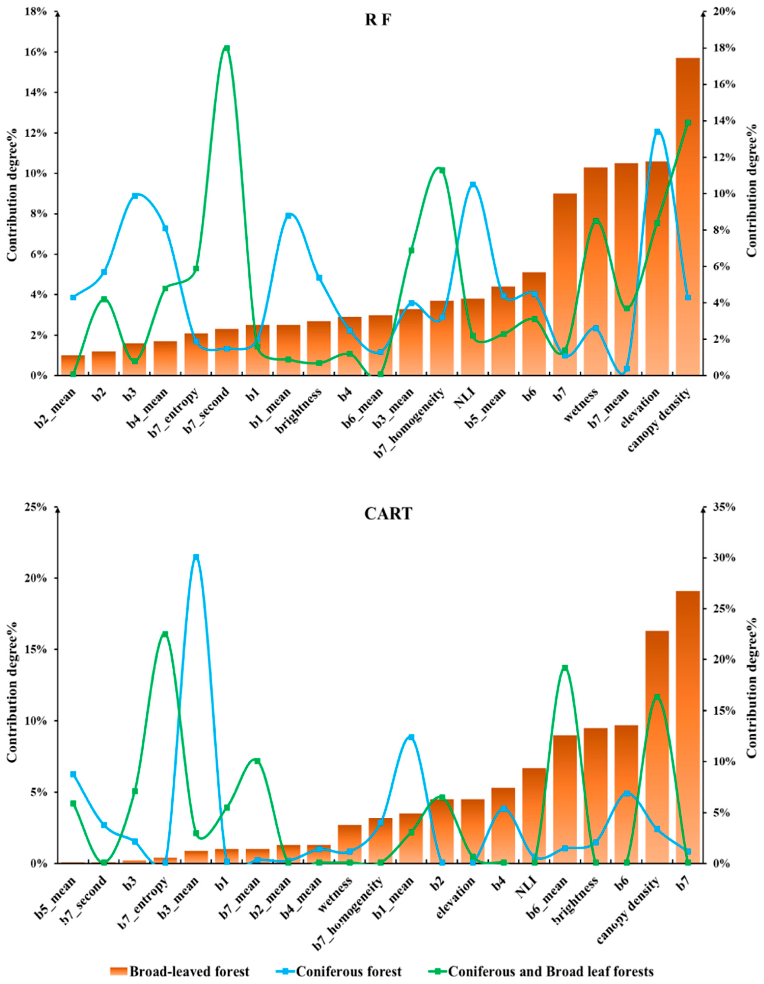
Yunnan Province is located between 21°8′–29°15′ N and 97°31′–106°11′ E, with a total area of 394.1 thousand km2. The topography features high in the northwest and low in the southeast, exhibiting a characteristic step-like descent from north to south. It is primarily a mountainous plateau region, with mountainous areas accounting for 88.64% of the province’s total area. The terrain is divided into two major topographic zones, eastern and western, demarcated by the Yuanjiang Valley and the southern part of the Yunling Mountain Range. The western and southern boundaries of the study area share borders with Vietnam, Laos, and Myanmar, while its northern and eastern boundaries adjoin Guangxi, Guizhou, Sichuan, and Tibet [19]. The province boasts rich and diverse forest vegetation, which is categorized into four primary forest vegetation types, 17 subtypes, and 105 forest types in total. Yunnan is renowned for having the highest plant species diversity in China and is often referred to as the ‘Kingdom of Plants’, Based on data from the Ninth National Forest Resources Inventory of China, as of the year 2021, the total forest area in the province measures 21.0616 million hectares, with a forest stock volume of 1.973 billion cubic meters and a forest coverage rate of 55.04% [20]. The geographical location of the study area is depicted in Figure 1.

Figure 1.
Overview of the study area and distribution of sample plots.
2.2. Data Acquisition and Preprocessing
2.2.1. Remote Sensing Image Acquisition and Preprocessing
The research utilizes the USGS Landsat 8 Level 2, Collection 2, Tier 1 dataset from the GEE platform database as the source of Landsat 8 satellite image data. After careful consideration and obtaining high-quality Landsat 8 image data, we utilized the median of all available satellite image data from June to December 2021, resulting in a composite satellite image with a cloud cover of less than 20%. The data collection period for the continuous forest inventory in Yunnan Province in 2021 was from September to December, which is not significantly different from the dates of the Landsat 8 images used (June to December 2021), indicating no significant time gap between the Landsat 8 dates and the field reference data. All “data” products are created with a single-channel algorithm jointly created by the Rochester Institute of Technology and National Aeronautics and Space Administration Jet Propulsion Laboratory.
The Digital Elevation Model (DEM) data utilizes the NASA NASADEM Digital Elevation 30 m as the source of DEM data, which is a digital elevation model released by the National Aeronautics and Space Administration, with a resolution of 30 m. This data is a reprocessing of STRM data, with improved accuracy by incorporating auxiliary data from “ASTER GDEM” “ICESat GLAS” and “PRISM” datasets. The selected Landsat 8 data products have undergone orthorectification and atmospheric calibration, so this study will not repeat the above operations, only performing cloud removal, fusion, and cropping of images.
2.2.2. Acquisition and Processing of Ground Survey Data
The ground survey data used in this study are from the continuous forest resource inventory data of Yunnan Province conducted by the Southwest Survey and Planning Institute of the National Forestry and Grassland Administration from September to December 2021. A total of 1072 fixed sample plots with a square area of 800 m2 were surveyed. The geographic coordinates of the center points of the sample plots were obtained through differential GPS survey. The survey data include detailed information on dominant tree species (groups), biomass, and origin. As this study did not involve the carbon storage of shrubs, the understory, herbaceous layer, litter layer, or soil layer, the carbon storage of these layers is not included in this study. In accordance with the technical regulations outlined in the ‘Main Technical Specifications for Forest Resource Planning and Design Survey’ (forest resources development (2003) 61) issued by the State Forestry and Grassland Administration of China, and considering the research scope and practical considerations, the forest classification types were ultimately determined to be broadleaf forests, coniferous forests, and mixed broadleaf-conifer forests, comprising a total of three categories. Specific sample category information can be found in Table 1.

Table 1.
Type and number of sample plots surveyed.
Utilizing high-resolution Google Earth imagery from the year 2021, a visual interpretation was conducted in Yunnan Province, China. The sample selection criterion employed was random sampling, and a total of 460 non-forest sample points were chosen. The dataset used for training the classification model consists of 1532 sample points, comprising field survey data and visual interpretation data, as illustrated in Figure 1 to depict their distribution.
2.2.3. Calculation of Aboveground Carbon Storage
Forest stock volume is the comprehensive outcome of forest growth, as current research conducted by most scholars indicates there exists a significant correlation between forest biomass and stock volume. The method for estimating forest carbon storage based on the relationship between biomass and accumulation is a direct and efficient approach, which has been widely applied in recent years for the estimation of forest carbon storage.
Based on the acquired sample plot standing volume, it is multiplied by the Biomass Expansion Factor to obtain the aboveground biomass of the sample plot. To facilitate calculations, the sample plot biomass is converted into biomass per hectare (t·hm−2). Multiplying the biomass per hectare by the corresponding carbon content ratio yields the aboveground carbon stock of the sample plot. The BEF is derived from the Yunnan Province tree species (group) BEF data provided by Tu Hongtao [20]. Biomass relationship equations for various dominant tree species (groups) are estimated as presented in Table A1 (Appendix A). Currently, in most domestic research, an average carbon content rate of 0.5 or 0.45 is used to estimate forest carbon stocks. However, due to variations in carbon content coefficients among different tree species (groups), a fixed carbon content rate for estimating carbon stocks may result in reduced precision. Therefore, in this study, calculations were conducted China’s “Guidelines for Carbon Sequestration Measurement and Monitoring in Afforestation Projects (LY/T 2253-2014)” and the research findings of relevant scholars [21,22,23]. For tree species (groups) for which carbon content has not been directly measured, a reference approach was employed by substituting carbon content rates from similar tree species (groups).
2.3. Research Methodology
2.3.1. Selection and Analysis of the GEE Classification Algorithm
In alignment with the actual circumstances of the research area, this study utilizes classification algorithms offered by the GEE cloud platform. Specifically, four distinct classifiers RF, CART, GBT, and SVM are employed for comprehensive image classification procedures.
2.3.2. RF
RF achieves classification by constructing an ensemble of classification or regression trees, thereby mitigating the risk of model overfitting [24]. RF requires users to make decisions about two tuning parameters: the number of trees to grow and number of variables to randomly sample as candidates at each split. Through parameter tuning, we successfully prevented the occurrence of local optima in the classification results. After conducting numerous experiments to strike a balance between model performance and efficiency, we ultimately decided to set the number of grown trees to 150. The minimum number of samples in a leaf node is set to 1, while the remaining parameters are kept at their default values. The RF classification model was implemented using the ‘smileRandomForest’ package in GEE, while the RF regression algorithm was implemented using the ‘RF Regressor’ package in the Python programming language.
2.3.3. CART
The CART algorithm, introduced by Breiman and his colleagues in 1984 [25], is an efficient regression method that does not require parameters for classification. The CART algorithm continuously divides the training sample set, calculates the GINI coefficient for each split point, and selects the one with the smallest GINI coefficient as the threshold for that split point. After threshold division is performed using the GINI coefficient, complex and large-scale decision trees are formed. In this study, we set the number of trees to 120, the minimum number of samples in a leaf node to 1 and kept the remaining parameters at their default values. The CART classification model was implemented using the “ee.Classifier.cart” function within GEE, While the CART regression algorithm was implemented using the ‘Scikit-learn’ package in the Python programming language.
2.3.4. GBT
The GBT algorithm employs regression decision trees as weak classifiers. The optimization of the regression decision tree primarily relies on the leaf node splitting process. By comparing the difference in loss values before and after the split between child nodes and parent node, the optimal split point is identified, which in turn minimizes the classifier’s loss and maximizes the difference between the split node and child nodes. In this study, the optimal classification performance is achieved when the number of trees is set to 100, the learning rate is set to 0.2, and the depth of each tree is set to 3, with the remaining parameters at their default values. The GBT classification model was implemented using the “ee.Classifier.smileGradientTreeBoost” function within GEE.
2.3.5. SVM
The SVM algorithm, introduced in 1964, is a supervised classification method [26] renowned for its robust data analysis and pattern recognition capabilities. It finds extensive applications in the fields of remote sensing image classification and fusion, SVM utilizes the hinge loss function to calculate the empirical risk and incorporates a regularization term into the calculation system to optimize the structural risk. In this study, the radial basis function was employed as the kernel function for the SVM, requiring the determination of two parameters: the regularization parameter ‘cost’ and the kernel function parameter ‘gamma’. Optimal values, determined through iterative testing, were identified as cost = 10 and gamma = 0.5. The SVM classification model is implemented using the “ee.Classifier.libsvm” function in GEE.
2.4. Feature Factor Selection
2.4.1. Selection of Feature Factors for GEE Classification
The quality of remote sensing image classification is closely tied to the selection and application of feature factors. Choosing and applying these feature factors can reduce inter-feature correlations, maximize the inclusion of original image information in fewer bands, and notably enhance the final classification results. Utilizing the GEE platform, a feature dataset is constructed, based on the original spectral features, incorporating texture features and terrain factors, among others. After repeated comparisons with related literature [27,28], a final selection of 29 feature factors was made, which includes 7 bands, 3 components of the hood transformation, 10 vegetation indices, and 9 texture features that participate in the classification.
2.4.2. Selection of Modeling Feature Factors
To construct a carbon stock estimation model, the consideration of modeling factors is of primary importance. In this study, we rely on Landsat 8 imagery and DEM data, incorporating spectral information, vegetation indices, Tasseled Cap Transformation, terrain factors, and textural features as characteristic variables. The three extracted terrain features, seven original band features, ten vegetation index features, three components of the Tasseled Cap Transformation, and 56 texture features from the gray level co-occurrence matrix are used [29]. The feature factors and related formulas can be found in Table A2 (Appendix A).
2.5. Construction of Forest Aboveground Carbon Storage Estimation Model
In this study, a random sample of 70% of the data was used for modeling through multiple linear regression and RF methods, while the remaining 30% of the data was reserved for accuracy validation. By employing data filtering, we ensured that the plots utilized for accuracy validation are spatially non-adjacent to the plots employed during model training. Yunnan Province’s forest ecosystem is categorized into three distinct types: broadleaf forests, coniferous forests, and mixed broadleaf-coniferous forests. Subsequently, construct models for each forest type using multiple linear stepwise regression, RF regression, and decision tree regression. In this study, it is worth noting that the modeling factors used for the three regression models remain consistent. The Pearson correlation coefficient analysis method was employed to conduct variable selection for the independent variables, identifying highly significant variables.
Multivariate Linear Models
When a linear relationship exists between multiple independent variables and the dependent variable, the regression analysis performed is referred to as a multivariable linear regression model. The selected independent variables are then used in the construction of a stepwise multivariable linear regression model [30]. The Variance Inflation Factor (VIF) method was employed to address the issue of multicollinearity among variables. The VIF, or Variance Inflation Factor, is defined as the ratio of the variance when there is multicollinearity among explanatory variables to the variance when multicollinearity is absent. It serves as the reciprocal of tolerance, where a higher VIF value indicates a more severe level of multicollinearity [28]. Based on the pertinent literature sources [31,32], this study establishes the criteria of 0 < VIF < 10 and tolerance > 0.1 for control and further selection of independent variables. At the 0.01 significance level, variables demonstrating consistent significance were chosen as independent variables. A multivariable stepwise regression model was established for the relationship between forest aboveground carbon storage and its characteristic factors, with entry criteria based on the T-test reaching a significance level of p < 0.05 [33]. The modeling equation for the multivariable stepwise regression method is represented as Equation (1).
where represents the sample biomass, signifies the selected modeling factors, denotes the regression coefficients, and corresponds to the constant term within the equation.
2.6. Model Validation and Accuracy Assessment
2.6.1. Evaluation of Classification Accuracy for GEE
In this study, the research area was classified into seven categories: broadleaf forest, coniferous forest, mixed coniferous and broadleaf forest, water bodies, built-up areas, cultivated land, and other types, with a total of 1532 samples. These samples comprise 557 from broadleaf forests, 365 from coniferous forests, 150 from mixed coniferous and broadleaf forests, 90 from water bodies, 120 from built-up areas, 120 from cultivated land, and 130 from the ‘other’ category. Of these, 70% were used as training samples, and 30% were allocated as validation samples. Various classification algorithms, including the RF algorithm, the CART, the GBT algorithm, and the SVM algorithm, were employed for the categorization of the study area.
The classification results were assessed for accuracy using a confusion matrix. To validate the reliability of the classification results, various evaluation metrics, including the overall accuracy (OA) and Kappa coefficient, were computed using a confusion matrix [34]. The overall classification accuracy and the Kappa coefficient were employed to assess the global classification performance. The formulas for computing the overall classification accuracy and the Kappa coefficient are as follows:
where stands for the number of pixels in the classified results that correspond to the actual land cover; represents the diagonal elements; represents the total sample count; and denote the summation of the matrix’s row and column, respectively.
2.6.2. Model Validation and Accuracy Assessment for Carbon Stock Estimation
To assess the reliability of the model, an evaluation of its predictive accuracy was conducted. This evaluation involved the utilization of validation sample data in both the context of multiple linear regression and RF regression models. The resultant predictions made by the model were then compared against the actual measured values, serving to gauge the model’s estimation performance within the study. The evaluation metrics used in this study include the coefficient of determination (R2), RMSE, rRMSE, and MAE. These metrics are utilized to gauge the model’s precision. A higher R2 indicates better model fit, whereas lower values of RMSE, rRMSE, and MAE signify a higher prediction accuracy of the model. The computation formulas for the three evaluation metrics are as follows:
where represents the sample data size, denotes the observed carbon storage values, signifies the predicted carbon storage values, and represents the mean of the observed carbon storage values.
2.7. Method Implementation
The GEE platform was employed for the classification processing of the research area; ArcGIS 10.8 was utilized for the extraction of altitude, slope, and aspect; ENVI 5.6 was used to extract factors such as vegetation indexes, Tasseled Cap Transformation, texture information, etc.; SPSS26.0 was applied for Pearson correlation analysis, feature screening, and the establishment of multivariable linear stepwise regression models for the three types of forests. Python3.11 was used for the establishment of RF regression models for the three types of forests and the inversion of carbon storage.
3. Results
3.1. Classification Results and Accuracy Evaluation
3.1.1. Classification Results
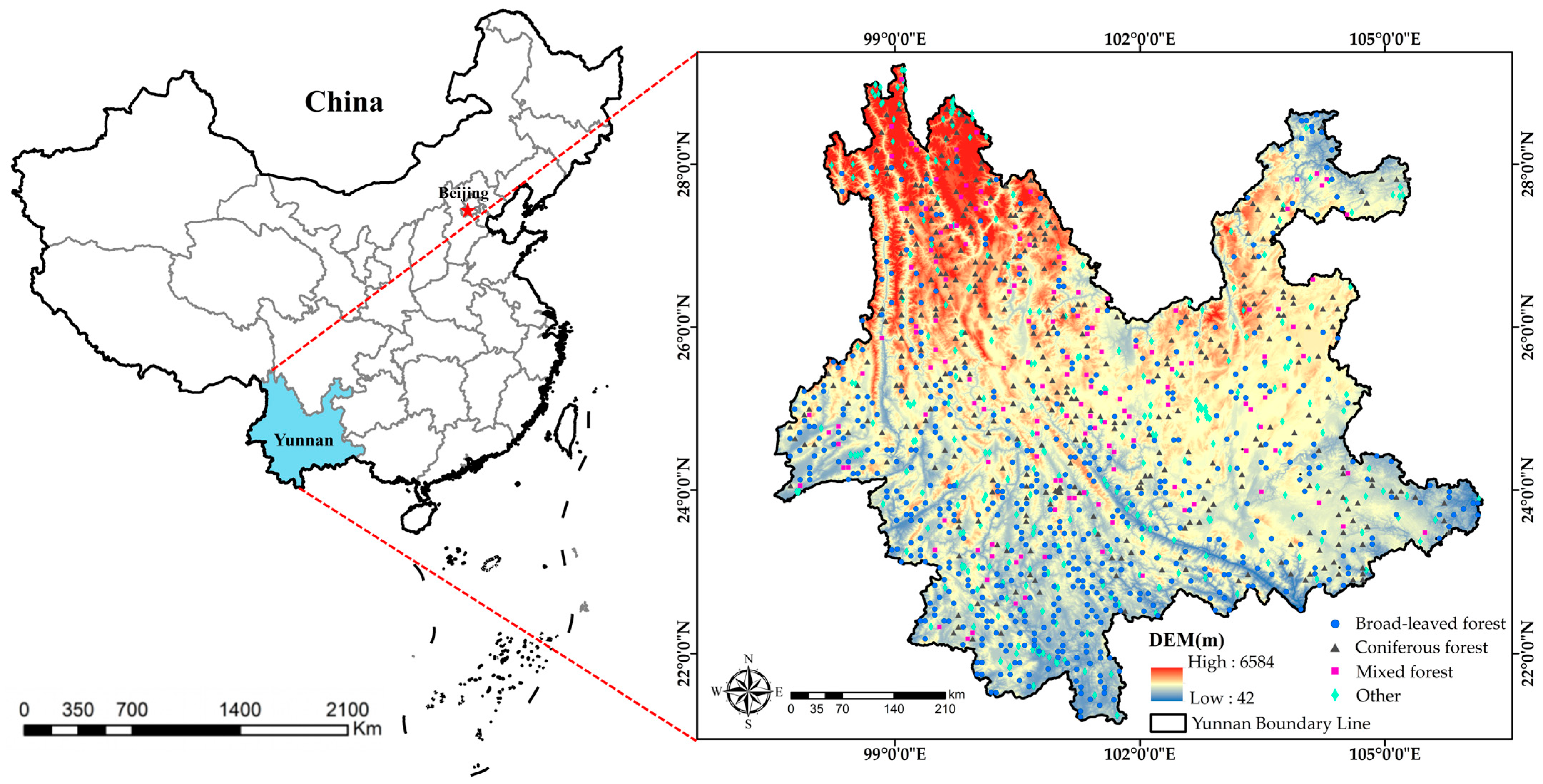
To achieve improved classification performance, this study conducted comparative experiments on five different feature combination schemes (Figure 2a–e). In the initial set of experiments, seven spectral features were utilized for classification with four different algorithms. Subsequent experiments expanded upon this initial set by incorporating additional factors for classification. The inclusion of other feature factors alongside spectral features led to varying degrees of improvement in overall accuracy (OA) and Kappa coefficients, as indicated in Figure 3. When utilizing only the spectral band feature, the overall accuracies of the RF, CART, GBT, and SVM algorithms are 0.7165, 0.6813, 0.7130, and 0.6127, respectively, with Kappa coefficients of 0.6147, 0.5672, 0.6068, and 0.4781 (Figure 2a). In contrast, incorporating five features, namely spectral bands, vegetation index, texture, principal component analysis, and terrain, enhances the overall accuracies to 0.8496, 0.8133, 0.8273, and 0.7315 for the RF, CART, GBT, and SVM algorithms, accompanied by Kappa coefficients of 0.7646, 0.7186, 0.7320, and 0.6388, respectively (Figure 2e). Upon the inclusion of vegetation index features, four algorithms exhibited an upward trend in both overall accuracy and Kappa coefficients (Figure 2b). However, with the incorporation of texture features, a notable decrease was observed in the overall accuracy and Kappa coefficients for four algorithms (Figure 2c). Subsequently, upon the addition of principal component analysis and terrain features, there was a varying degree of improvement in both overall accuracy and Kappa coefficients for the four algorithms (Figure 2d,e). When applying the SVM classifier, it exhibited relatively poorer performance in comparison to other classifiers, with an overall accuracy of 0.7315 and a Kappa coefficient of 0.6388.
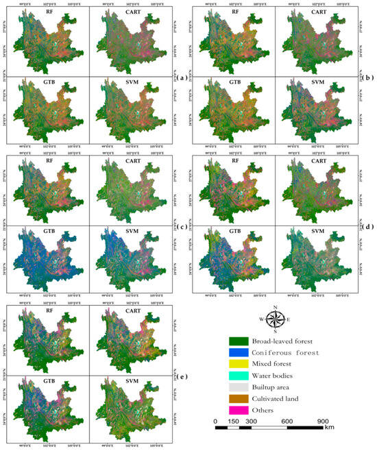
Figure 2.
Classification results based on four algorithms of the GEE platform (a) Spectral features (b) Spectral and vegetation index features (c) Spectral, vegetation index, and texture features (d) Spectral, vegetation index, texture, and principal component analysis features (e) Spectral, vegetation index, texture, principal component analysis, and terrain features.

Figure 3.
Comparison of overall accuracy and Kappa coefficient of different classification algorithms with different features (a) Spectral features (b) Spectral and vegetation index features (c) Spectral, vegetation index, and texture features (d) Spectral, vegetation index, texture, and principal component analysis features (e) Spectral, vegetation index, texture, principal component analysis, and terrain features.
Among the four classification algorithms, the RF algorithm exhibited superior performance, with an overall accuracy of 0.8496 and a Kappa coefficient of 0.7646. Therefore, this study relies on the classification results obtained through the RF algorithm to estimate the aboveground carbon stock in Yunnan Province’s forests. The classification results of the four algorithms are shown in Figure 2.
3.1.2. Accuracy Assessment
The classification results of four different classification algorithms are evaluated for precision using the Confusion Matrix method. The results from the Error Matrix for each classification algorithm are presented in Figure A1 (Appendix A).
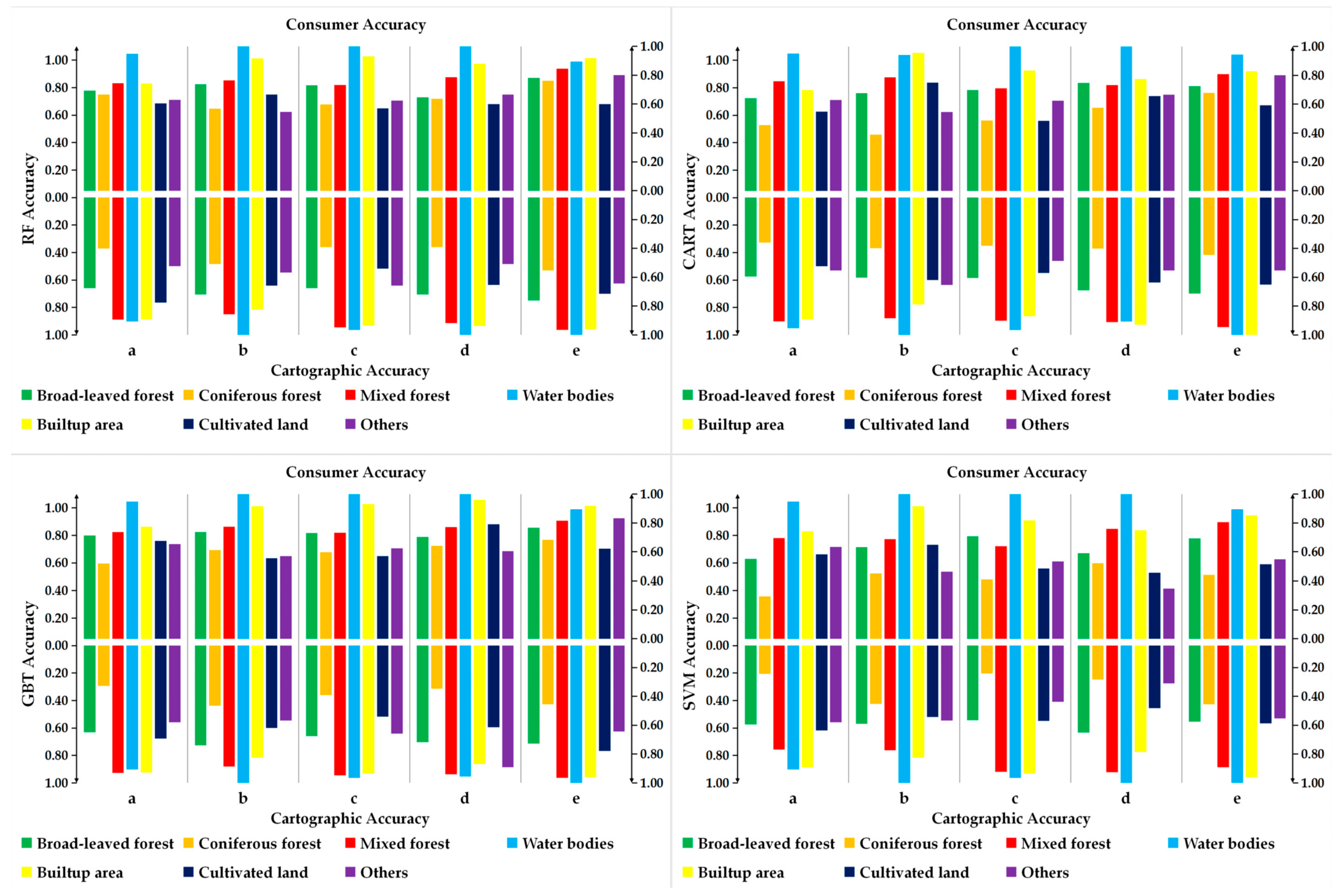
According to Figure 4, it is evident that the RF algorithm outperforms other machine learning algorithms in terms of Cartographic Accuracy and Consumer Accuracy. Therefore, the RF algorithm is more suitable for the classification of forest types in Yunnan Province than other machine algorithms.

Figure 4.
Comparison of Cartographic Accuracy and Consumer Accuracy using different features and classification algorithms (a) Spectral features (b) Spectral and vegetation index features (c) Spectral, vegetation index, and texture features (d) Spectral, vegetation index, texture, and principal component analysis features (e) Spectral, vegetation index, texture, principal component analysis, and terrain features.
3.2. Analysis of Model Variable Correlation
The Pearson correlation coefficient signifies the linear correlation degree between two model variables. The greater the absolute value, the stronger the correlation. Variables highly correlated with carbon storage are shown in Figure A2 (Appendix A). Out of the selected 80 independent variables, there are 21 variables demonstrating a very significant correlation (0 < p < 0.01) with carbon storage. In terms of band spectral characteristics, the carbon storage negatively correlates significantly with bands b1–b7 at the 0.01 level. Carbon storage positively correlates significantly with canopy density and elevation at the 0.01 level. Carbon storage is significantly correlated with all other independent variables at the 0.01 level.
3.3. Estimation of Aboveground Carbon Stock in Forests
Seventy percent of the plot data were used to build multivariate stepwise regression, RF regression, and decision tree regression models for carbon stock estimation. The remaining thirty percent of the data was allocated for model accuracy validation.
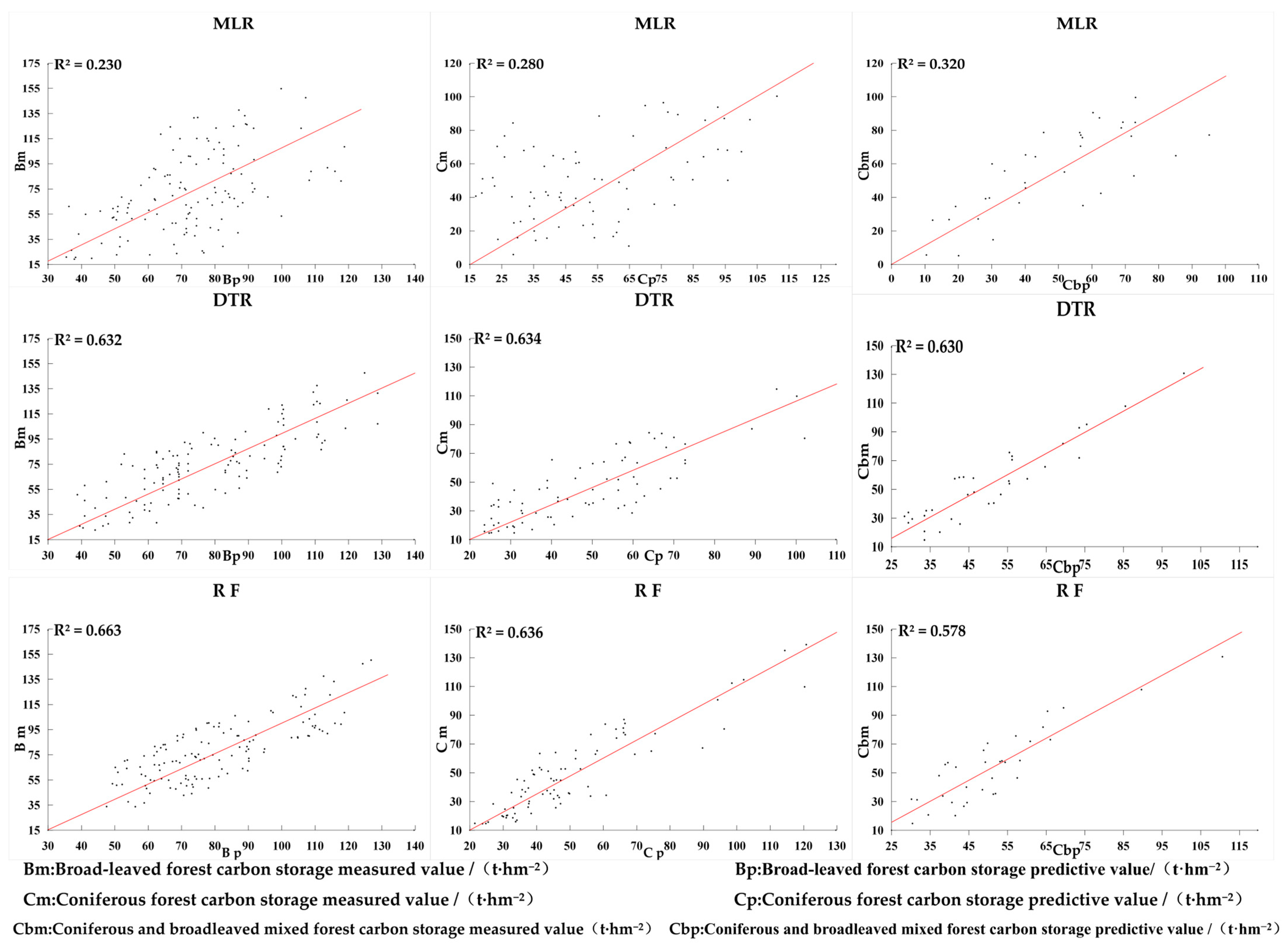
Utilizing sample data on carbon stock for various forest types and 21 highly correlated modeling factors, optimal models for aboveground carbon stock in different forest types were constructed using multivariate stepwise regression, RF regression, and decision tree regression methods. RF and decision tree rank input factors based on their importance and provide modeling contribution values for each factor. The contribution percentages of modeling factors for three forest types in this study are depicted in Figure A3 (Appendix A). The results of the three regression models, obtained after tuning model parameters, are illustrated in Figure 5.
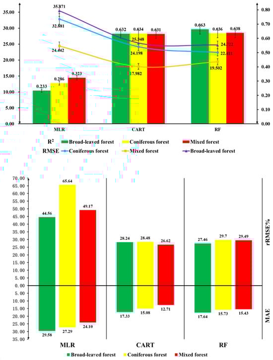
Figure 5.
Modeling results of three regression models.
The accuracy of the carbon storage estimation model is assessed using metrics such as the coefficient of determination (R2), relative root mean square error, mean squared error, and mean absolute deviation, derived from the computed values predicted by multivariate linear stepwise regression, RF regression, and decision tree regression models. From Figure 5, it is evident that the coefficient of determination (R2) for the broad-leaved forest model under the multivariate linear stepwise regression framework is relatively low, amounting to 0.23. The RMSE, rRMSE, and MAE for the same are 35.471, 32.881, and 24.442, respectively. The coefficient of determination (R2) for all three forest types is less than 0.4, indicating that the values of RMSE, rRMSE%, and MAE are comparably larger. In the RF regression model, the coefficient of determination (R2) for the broad-leaved forest model is 0.663 with an RMSE of 24.722, rRMSE of 27.46, and a MAE of 17.64. For both coniferous and mixed forests, the coefficient of determination (R2) is above 0.6, with R2 values exceeding 0.6 for both RF and decision tree models, indicating good fitting efficacy for both models. After a detailed comparison, the RF model outperforms the decision tree model. Consequently, this study employs the RF regression model to estimate the above-ground carbon storage in Yunnan Province’s forests. Accuracy validation was conducted using the actual values from the remaining 30% of broad-leaved, coniferous, and mixed forests. The performance of the model can be interpreted with a scatter plot, which shows the relationship between the actual carbon stock values and the predicted carbon stock values (Figure 6). According to the scatter plot, the performance of both RF and decision tree models is superior to that of the Multivariate Linear model under the same dataset.
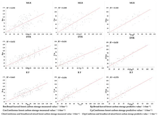
Figure 6.
Comparison of measured and predicted carbon stock values for three models.
3.4. Spatial Distribution Characteristics of Aboveground Carbon Stock in Yunnan Province’s Forests
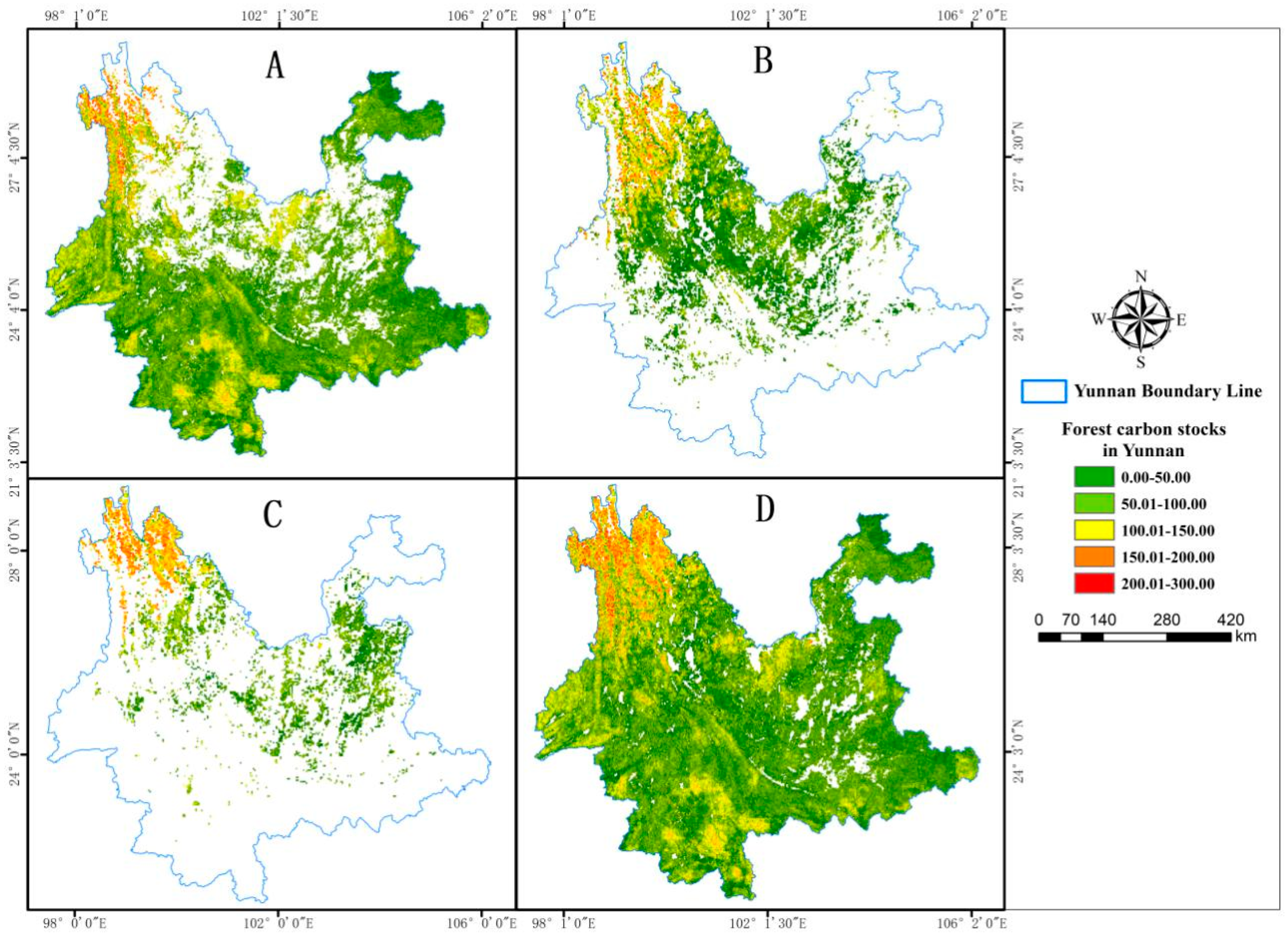
In accordance with the RF regression model, the estimated distribution maps of carbon storage in Yunnan Province’s broad-leaved forest (Figure 7A), coniferous forest (Figure 7B), mixed forest (Figure 7C), and overall forest (Figure 7D) have been derived.
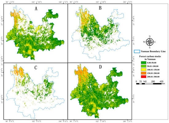
Figure 7.
Distribution map of carbon stock in Yunnan Province’s forests (A) Carbon stock distribution map of broadleaved forests in Yunnan Province (B) Carbon stock distribution map of coniferous forests in Yunnan Province (C) Carbon stock distribution map of mixed forests in Yunnan Province (D) Carbon stock distribution map of forests in Yunnan Province.
From Figure 7, it is evident that the carbon stock of broadleaf forests is relatively high (approximately 100–200 t·hm−2) in the high-altitude regions of southern Yunnan Province, encompassing Puer, Xishuangbanna, Dehong, and the Nujiang Gorge area. This phenomenon can be primarily attributed to the fact that these regions are situated in the southern tropical zone of China, characterized by abundant rainfall, an extended frost-free period throughout the year, and favorable temperatures, all of which are conducive to the growth of broadleaf forests. Furthermore, the complex topography and the presence of vast forested landscapes in these areas, such as tropical rainforests, seasonal rainforests, and montane rainforests, contribute to the higher carbon stocks observed. Additionally, these regions experience relatively lower anthropogenic disturbances and reduced human activities, often resulting in greater carbon stocks when compared to more developed areas. The carbon stock in coniferous forests is significantly higher in the northern regions of Yunnan, particularly in the northwestern areas of Yunnan, where coniferous forests comprise a substantial portion of the land cover, resulting in higher carbon stocks, ranging between 100 and 250 t·hm−2. However, assessing the carbon stock in the Puer region of Yunnan is hindered by limited field data for coniferous forests and the uncertainties introduced by classification errors, leading to suboptimal estimates in this specific area. Mixed coniferous and broadleaf forests are relatively scarce in distribution across the entire province, with carbon stocks being uniformly distributed within the range of approximately 50 to 150 t·hm−2. Broadleaf forests exhibit both higher per-unit volume and per-unit biomass than coniferous forests, resulting in superior carbon sequestration capabilities and overall carbon stocks. In general, broadleaf forests play a more significant role in carbon sequestration within the forest vegetation of Yunnan Province compared to coniferous forests. When compared to mixed coniferous and broadleaf forests, broadleaf forests exhibit larger areas and higher carbon stocks. Therefore, in the context of expanding forested areas and increasing forest carbon stocks, it is advisable to consider an appropriate increase in the extent of broadleaf forests. Figure 7D shows that the distribution of forest carbon stocks in Yunnan Province is both widespread and predominantly concentrated in the northwestern and southwestern regions, following a pattern of higher values in the south and lower values in the north, with a west-to-east decline.
By overlaying the aboveground carbon stock distribution in the forests of Yunnan Province with DEM data, distinct carbon stock scenarios can be obtained for different elevation gradients, slopes, and aspects, as illustrated in Figure 8. In the vertical space, the carbon stock of broad-leaved forests is primarily distributed within the altitude range of 1500 to 2000 m, accounting for 32.47% of the total aboveground carbon stock of broad-leaved forests in Yunnan Province. The carbon stock of coniferous forests is predominantly situated in regions above 2000 m elevation, while the carbon stock of mixed coniferous and broad-leaved forests is mainly located in areas above 2500 m, constituting 42.60% of the total aboveground carbon stock of mixed forests in Yunnan Province. Overall, the carbon storage of forests in Yunnan Province is mainly concentrated in areas above 1500 m. In terms of slope, the carbon stock in the forests of Yunnan Province is predominantly distributed within the 10–30° range, accounting for 60.95% of the total aboveground carbon stock in Yunnan’s forests. Regions with slopes exceeding 40° exhibit lower proportions of forest carbon stock due to the steeper incline. Moreover, aside from areas without a specific slope direction where the carbon stock proportion is relatively minor, the distribution disparities of aboveground carbon stock in the forests of Yunnan Province among various slope directions are comparatively small, with distinctions not being prominently evident.
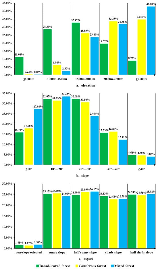
Figure 8.
Proportion of carbon stock in different forest types based on varying elevations, slopes, and aspects.
4. Discussion
Machine learning, as a focal point in the remote sensing field, holds significant importance in addressing the challenges of vast remote sensing data and the time-consuming nature of traditional visual interpretation. Numerous machine learning algorithms are extensively employed for the classification of remote sensing imagery [35,36,37]. However, enhancing the classification performance of machine learning algorithms is emerging as a significant topic of discussion among numerous research scholars. Ghimire [38] incorporates the GETIS statistic as a feature variable into the RF classification model, thereby enhancing the classification performance of the RF algorithm. The resulting Kappa coefficient accuracy ranges from 0.85 to 0.92. Duro et al. [39], following parameter optimization, conduct a comparative analysis of three machine learning algorithms: decision trees, RF, and SVM. The results indicate that RF and SVM exhibit a competitive edge in agricultural landscape classification, with higher overall accuracy and Kappa coefficients when compared to decision trees.
The optimization of model parameters is of particular importance for non-parametric models. In the context of RF, the subsampling rate is a crucial parameter for adjusting both the model’s performance and its robustness [40]. The choice of subsampling rate has the potential to significantly impact the model’s performance and training speed. A higher subsampling rate can reduce training time but may potentially result in model underfitting. Conversely, a lower subsampling rate may prolong training time, yet it aids in alleviating overfitting issues. Freeman et al. [41] found that the optimal model’s subsampling rate was approximately 0.5, while Elith et al. [42] suggested choosing a value between 0.5 and 0.75. In contrast, the RF optimization model in this study demonstrates better performance when utilizing a subsampling rate of 0.7. Regarding the number of trees, Probst et al. [43] advocated setting this parameter as high as possible, while Liaw et al. [44] research findings suggested that, after a specific number of trees, the model’s stable accuracy effectively represents its performance. In the present study, when the number of trees was increased by 150 in the classification algorithm, the RF classification model exhibited improved performance with higher accuracy, and overfitting was less likely to occur. In CART and GBRT models, setting the number of trees to 120 and 100, respectively, yields satisfactory classification performance. In the context of SVM, the key parameters that influence model performance are the regularization parameter “cost” and the radial basis function parameter “gamma.” In this study, a radial basis function (RBF) was used as the SVM kernel function because Rodriguez-Galiano et al. [45] indicated that RBF was superior to linear, polynomial and sigmoid functions. A larger “gamma” value may lead to overfitting, while a higher “cost” value can result in the classifier emphasizing correct classification of the training data, potentially causing overfitting [46]. Therefore, after repeated testing, we ultimately determined that a “cost” value of 10 and a “gamma” value of 0.5 yielded the best classification performance.
Most early studies on biomass and carbon storage estimation were based on classical statistical regression methods, such as linear regression, which assumes a linear relationship between the predictor and predicted variables [47,48]. Nevertheless, the connection between forest carbon storage and remote sensing data is highly intricate, and conventional statistical regression methods fall short in comprehensively elucidating this intricate relationship machine learning algorithms such as RF can effectively establish intricate nonlinear relationships between remotely sensed image data with uncertain distributions and vegetation information. Moreover, they exhibit versatility in integrating data from diverse sources, thereby enhancing predictive accuracy [49,50]. Yingchang Li et al. [51] conducted a comparative analysis for estimating biomass in subtropical forests using three algorithms: Linear Regression, RF, and Extreme Gradient Boosting. The research findings reveal that the XGBoost model achieved an R2 value of 0.75. Safari [52] employed multi-temporal Landsat 8 spectral data to assess carbon stock in upland Quercus semecarpifolia Sm. forests using four machine learning algorithms. The outcomes indicate that the RF algorithm generally exhibited robust results, with an R2 value of 0.66 and a root mean square error of 34.36. Numerous studies have demonstrated that the collaborative interaction between machine learning algorithms and remote sensing data can prevent overfitting and significantly improve predictive accuracy compared to the traditional LR model. Gao et al. [53] employed a variety of machine learning algorithms (K-Nearest Neighbors, Artificial Neural Networks, SVM, RF) for estimating above-ground biomass in subtropical forests. The results indicate that machine learning algorithms demonstrate robust performance in AGB estimation. Li et al. [54] employed Linear Dummy Variable Models and Linear Mixed-Effects Models to estimate biomass in the Xiangxi region of China. The R2 values for the entire vegetation set were 0.41, while the R2 for the combined dataset’s LR model was only 0.22. In contrast, results obtained in this study using the RF machine learning algorithm outperformed the LR model in terms of R2, RMSE, rRMSE, and MAE. This suggests that the RF algorithm demonstrates superior performance in carbon storage estimation, reducing the extent of underestimation and overestimation to a certain degree. It is worth noting that the issue of low values being overestimated and high values being underestimated when using machine learning algorithms has not been completely eliminated. This problem has also been observed in previous studies of non-parametric algorithms for carbon storage or biomass estimation [55]. The algorithm itself governs the determination of this. Moreover, a data saturation issue arises when estimating carbon stock using remote sensing data. Consequently, we conducted stratified estimation based on forest types, with the goal of minimizing potential estimation errors.
In most studies on forest carbon stock estimation, the focus is predominantly on the use of regression methods. Similarly, in studies related to land use classification, the emphasis is primarily on classification methods. Research that combines land use classification with forest carbon stock estimation is relatively scarce. This study combines various classification methods with regression techniques to estimate carbon stocks in different types of forests. Compared to traditional studies that focus solely on either land use classification or forest carbon stock regression, this approach represents a novel challenge. One of the advantages of machine learning in land use classification is that, compared to traditional statistical regression methods, machine learning is more suitable for handling the complex relationships between remote sensing data and vegetation information. This capability allows for more accurate land use classification. Through a comparative analysis of multiple algorithms, this study selects the Random Forest algorithm, which is most suitable for the current research objectives, and optimizes the algorithm parameters to improve classification accuracy and efficiency. Furthermore, achieving rapid land use classification is also a crucial issue. In this regard, this study employs data dimensionality reduction and feature selection to enhance the speed and efficiency of classification. Additionally, setting appropriate machine learning algorithm parameters can also influence the speed of classification to some extent, such as adjusting parameters like subsampling rate, number of trees, learning rate, etc., to achieve the goal of fast and accurate classification. In general, the more detailed the classification level, the richer the information it can provide. However, it also increases the complexity of classification and computational costs. When conducting land use classification, it is important to choose an appropriate classification level based on the research objectives and data availability. Therefore, this paper divides the study area into seven categories, with forests categorized into three groups, thereby improving the accuracy of forest carbon stock estimation. Overall, machine learning algorithms have clear advantages in land use classification. By optimizing algorithm parameters and appropriately dividing classification levels, it is possible to enhance the detail, speed, and accuracy of classification. This improvement makes machine learning algorithms more suitable for application in research and practice related to forest carbon stock estimation.
Furthermore, the study area is predominantly characterized by mountainous and hilly terrain, featuring significant variations in elevation. These elevation changes lead to shifts in temperature and precipitation with increasing altitude, resulting in a diverse range of vegetation forms within the study area. Therefore, remote sensing images exhibit rich and easily recognizable texture features, underscoring the undeniable importance of texture images [54,56]. It is notable that the spatial distribution characteristics in our study area align with the research of other scholars [57,58,59], indicating that constructing carbon storage estimation models for different forest types within a large-scale region leads to greater accuracy and better estimation of carbon sequestration values on a larger regional scale [60,61]. The primary strength of this study lies in the utilization of the GEE platform for image classification tasks. All four classification algorithms performed significantly faster than traditional software classification methods. Research has shown that using this method can significantly improve classification efficiency. Additionally, the GEE platform, which can be accessed freely, utilizes Landsat satellite data. The long-term, continuous, and cost-free nature of this data provides seamless global coverage of long temporal series surface reflectance, all of which contribute to considerably lowered usage costs. Another notable aspect of this study is the use of national continuous inventory data as classification samples, which enhances accuracy. This study classified the forests within the study area into three different types, thereby improving the accuracy of remote sensing estimation models. Certainly, research in the field does have certain limitations. In forest classification studies, numerous factors contribute to classification errors. The most significant factors leading to misclassification of forest types are the phenomena of “distinct spectra for the same object” and “the same spectra for different objects.” Additionally, the limitations of classification algorithms can introduce bias into the classification process. This study only utilized four machine learning algorithms, and while these four algorithms achieved relatively high classification accuracy, there some issues related to the misclassification of mixed pixels remained. In this study, forest above-ground carbon storage includes only the carbon stored in live trees and does not encompass the estimation of carbon storage in other components of the forest, such as shrubs, herbaceous vegetation, the litter layer, and the soil layer. Additionally, the study did not achieve a dynamic analysis of above-ground carbon storage in forest vegetation or predict its change trends over time.
The aforementioned study lays the foundation for future endeavors in predicting forest carbon stocks using continuous time series data. In the subsequent phase of our research, we plan to leverage the advantages of continuous temporal observations from Landsat satellites to further investigate the spatiotemporal dynamics of aboveground carbon storage in the forested regions of the area. Additionally, the ongoing updates and improvements in classification algorithms are expected to significantly boost the accuracy of forest classification.
5. Conclusions
This study utilized the Google Earth Engine cloud platform to acquire image feature parameters of forest vegetation in the study area through Landsat 8 satellite remote sensing data. Furthermore, it integrated on-site forest survey data. Using four different algorithms provided by the GEE cloud platform RF, CART, GBT, and SVM for image classification, the RF classifier exhibited the best performance. It achieved an overall accuracy of 84.96% and a Kappa coefficient of 76.46%. To account for the carbon sequestration capacity and carbon storage differences between different forest types, the modeling approach was refined. Multiple linear stepwise regression, RF regression, and decision tree regression models were separately established for broadleaf forests, coniferous forests, and mixed coniferous-broadleaf forests within the study area. The RF regression model exhibited the best performance, with an R2 value of 0.663 for the broadleaf forest model, an RMSE of 24.722, an rRMSE of 27.46, and a MAE of 17.64. For both coniferous and mixed forests, the coefficient of determination (R2) is above 0.6. With R2 values exceeding 0.6 for both RF and decision tree models, indicating good fitting efficacy for both models. The research results further demonstrate that combining machine learning classification results with forest carbon stock estimates at a large scale can yield satisfactory outcomes, providing a reference for rapid and accurate estimation of forest carbon stocks in other large-scale regions. Moreover, the research findings hold significant implications for ecological conservation and sustainable forest development in Yunnan Province, China. The order of above-ground carbon storage in different forest types in Yunnan Province is as follows: broadleaf forests > coniferous forests > mixed coniferous-broadleaf forests. This is not only related to the carbon sequestration capacity of different tree species but is also significantly influenced by the distribution area of each forest type. The carbon storage in Yunnan Province’s forests is predominantly concentrated in the northwestern and southwestern regions, with a pattern of higher carbon storage in the west and south and lower carbon storage in the north and east. Overall, the carbon storage of forests in Yunnan Province is mainly concentrated in areas above 1500 m. Regions with slopes exceeding 40° exhibit lower proportions of forest carbon stock due to the steeper incline. Moreover, aside from areas without a specific slope direction where the carbon stock proportion is relatively minor, the distribution disparities of aboveground carbon stock in the forests of Yunnan Province among various slope directions are comparatively small, with distinctions not being prominently evident.
Author Contributions
Writing—original draft preparation, formal analysis, F.C.; supervision, G.O.; investigation, M.W.; data monitoring and thesis revision, C.L. All authors have read and agreed to the published version of the manuscript.
Funding
Xingdian Talent Support Plan of Yunnan Province: YNWR-QNBJ-2019-064; Science and Technology Plan Project of Science and Technology Department of Yunnan Province: 202401AT070272.
Data Availability Statement
The sample plot data used in this study were derived from the 2021 National Forest Resource Inventory data in China, while Landsat 8 satellite imagery was sourced from the Google Earth Engine platform. It is important to note that Landsat 8 imagery is publicly available, whereas the 2021 National Forest Resource Inventory data is considered proprietary and not publicly accessible.
Conflicts of Interest
The authors declare no conflicts of interest.
Appendix A
Table A1.
The volume (V) and biomass (Y) relationship equation and carbon content rate of dominant tree species in Yunnan Province.
Table A1.
The volume (V) and biomass (Y) relationship equation and carbon content rate of dominant tree species in Yunnan Province.
| Number | Tree Species | Accumulation-Biomass Equation | Carbon Content (%) | Number | Tree Species | Accumulation-Biomass Equation | Carbon Content (%) |
|---|---|---|---|---|---|---|---|
| 1 | Abies fabri (Mast.) Craib. | Y = 0.4642V + 47.499 | 49.99 | 12 | Quercus L. | Y = 1.1453V + 8.5473 | 50.04 |
| 2 | Picea asperata Mast. | Y = 0.4642V + 47.499 | 52.08 | 13 | Betula L. | Y = 1.0687V + 10.237 | 49.14 |
| 3 | Keteleeria fortunei (Murr.) Carr. | Y = 0.4158V + 41.3318 | 49.97 | 14 | Schima superba Gardner & Champ. | Y = 0.7560V + 8.31 | 48.34 |
| 4 | Pinus armandii Franch. | Y = 0.5856V + 18.7435 | 52.25 | 15 | Liquidambar formosana Hance | Y = 0.7560V + 8.31 | 48.34 |
| 5 | Pinus yunnanensis Franch. | Y = 0.5101V + 1.0451 | 51.13 | 16 | Other hard-leaved broad-leaved trees | Y = 0.7560V + 8.31 | 48.34 |
| 6 | Pinus kesiya Royle ex Gordon | Y = 0.5101V + 1.0451 | 52.24 | 17 | Populus przewalskii Maxim. | Y = 0.4969V + 26.9730 | 49.56 |
| 7 | Pinus densata Mast. | Y = 0.517V + 33.238 | 50.09 | 18 | Eucalyptus robusta Sm. | Y = 0.8873V + 4.5539 | 52.53 |
| 8 | Other Pines | Y = 0.5168V + 33.2378 | 51.1 | 19 | Other soft-leaved broad-leaved species | Y = 0.4750V + 30.6030 | 49.56 |
| 9 | Cunninghamia lanceolata (Lamb.) Hook. | Y = 0.3999V + 22.541 | 52.01 | 20 | mixed broad-leaved forest | Y = 0.6255V + 91.003 | 49.0 |
| 10 | Cupressus funebris Endl. | Y = 0.6129V + 46.1451 | 50.34 | 21 | coniferous and broadleaved mixed forest | Y = 0.8019V + 12.2799 | 48.93 |
| 11 | mixed coniferous forest | Y = 0.5168V + 33.2378 | 51.68 |
Note: Y represents biomass per unit area in t/hm2; V represents volume per unit area in m3/hm2; carbon content rate is in percentage. Formula source: Tu Hongtao [20].
Table A2.
Carbon Stock Estimation Modeling Characterization Feature and Calculation Formulas and Sources.
Table A2.
Carbon Stock Estimation Modeling Characterization Feature and Calculation Formulas and Sources.
| Feature Types | Feature Names | Computational Formula |
|---|---|---|
| Vegetation Index | Normalized Difference Vegetation Index (NDVI) | |
| Normalized Water Index (NDWI) | ||
| Ratio Vegetation Index (RVI) | ||
| Difference Vegetation Index (DVI) | ||
| Ratio Vegetation Index 1 (RVI65) | ||
| Ratio Vegetation Index 2 (RVI75) | ||
| Soil-Adjusted Vegetation Index (SAVI) | ||
| Non-Linear Vegetation Index (NLI) | ||
| Atmospherically Resistant Vegetation Index (ARVI) | ||
| Enhanced Vegetation Index (EVI) | ||
| Texture characteristics | Mean | |
| Variance | ||
| Homogeneity | ||
| Contrast | ||
| Dissimilarity | ||
| Entropy | ||
| Second Moment | ||
| Correlation | ||
| Topographic features | Elevation, slope, aspect | DEM data extraction in the study area |
| Tasseled Cap Transformation | Brightness | GEE Platform Database Extraction |
| Greenness | ||
| Wetness | ||
| Band | Single-band | b1, b2, b3, b4, b5, b6, b7 |
Note: BLUE represents Band 2, GREEN represents Band 3, RED represents Band 4, NIR represents Band 5, SWIR 1 represents Band 6, and SWIR 2 represents Band 7. In the SAVI index, the L value is 0.5. Within the EVI index, the two correction coefficients for the gain factor G and the soil adjustment factor L, which are C1 and C2, are respectively 2.5, 0.10, 6.0, and 7.5. In the ARVI index, r is set to 1.0. Texture features are extracted using the gray level co-occurrence matrix from the seven bands b1–b7 of remote sensing imagery with a window size of 3 × 3. where denotes the pixel value at the row and column position. N signifies the size and dimension of the moving window. RVI65 and RVI75 represent the Ratio Vegetation Index of Band 6, Band 7, and Band 5, respectively. Source of vegetation index formula: Ren Yi et al. [27].

Figure A1.
Confusion matrices of four algorithms.
Figure A1.
Confusion matrices of four algorithms.
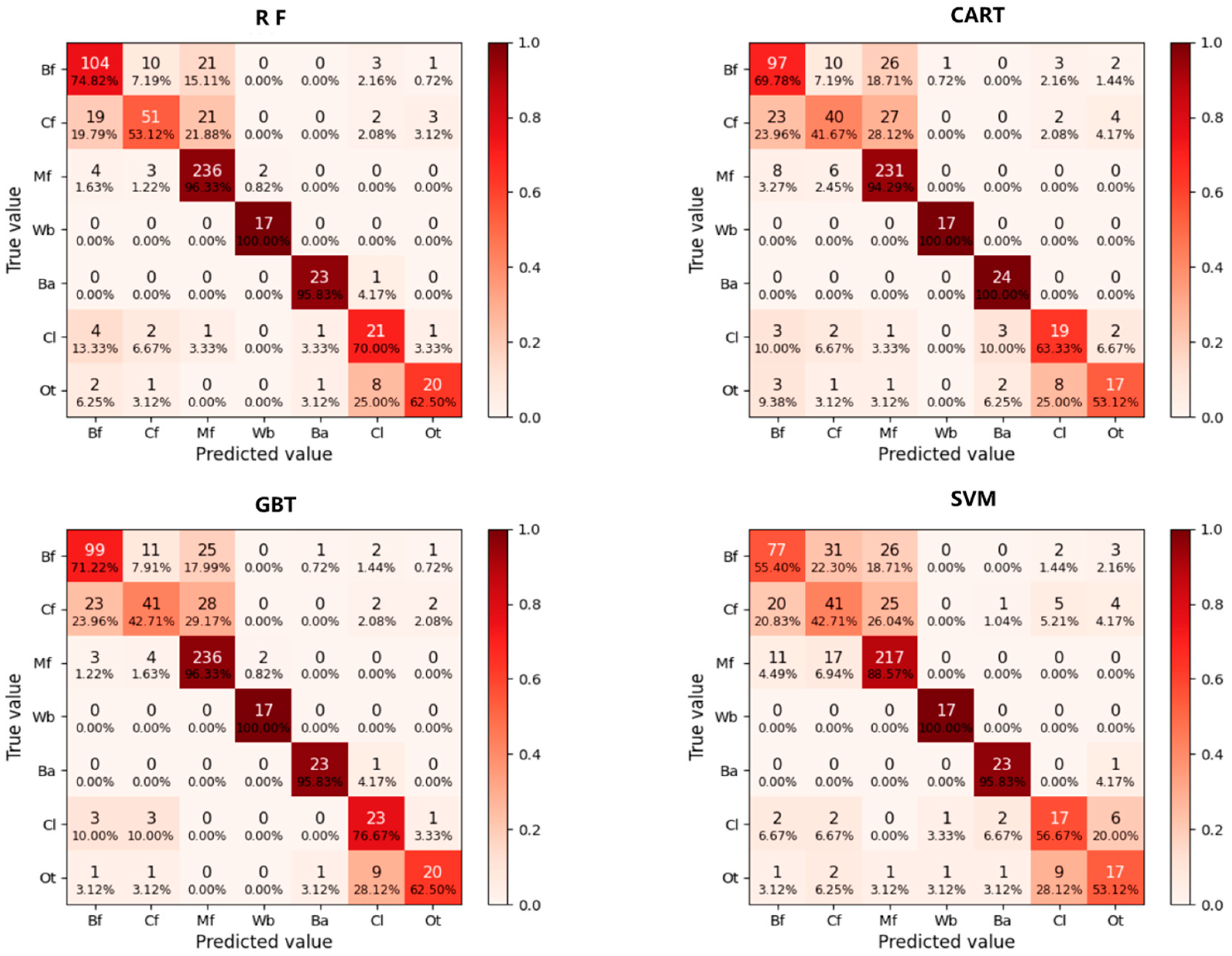
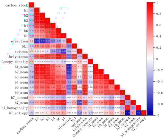
Figure A2.
Correlation between carbon stocks and 21 independent variables. Note: b1, b2, b3, b4, b5, b6, and b7 correspond to the 1st, 2nd, 3rd, 4th, 5th, 6th, and 7th bands of the Landsat 8 imagery, respectively. NLI stands for Non-linear Vegetation Index; ‘brightness’ and ‘wetness’ represent the tasseled cap transformation factors. ‘Mean’, ‘entropy’, ‘second’, ‘correlation’, ‘variance’, ‘contrast’ and ‘dissimilarity’ respectively represent Mean Texture, Entropy Texture, Second-Order Angular Moment Texture, Correlation Texture, Variance Texture, Contrast Texture, and Dissimilarity Texture.
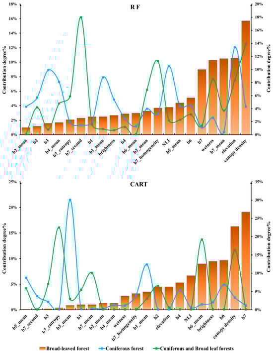
Figure A3.
Contribution Percentages of Modeling Factors for Different Forest Types in Two Models.
Figure A3.
Contribution Percentages of Modeling Factors for Different Forest Types in Two Models.
References
- Malhi, Y.; Baldocchi, D.D.; Jarvis, P.G. The carbon balance of tropical, temperate and boreal forests. Plant Cell Environ. 1999, 22, 453. [Google Scholar] [CrossRef]
- Abdollahnejad, A.; Panagiotidis, D.; Surovy, P.; Modlinger, R. Investigating the Correlation between Multisource Remote Sensing Data for Predicting Potential Spread of Ips typographus L. Spots in Healthy Trees. Remote Sens. 2021, 13, 4953. [Google Scholar] [CrossRef]
- Fassnacht, F.E.; Hartig, F.; Latifi, H.; Berger, C.; Hernández, J.; Corvalán, P.; Koch, B. Importance of sample size, data type and prediction method for remote sensing-based estimations of aboveground forest biomass. Remote Sens. Environ. 2014, 154, 102–114. [Google Scholar] [CrossRef]
- Zheng, D.; Heath, L.S.; Ducey, M.J. Spatial distribution of forest aboveground biomass estimated from remote sensing and forest inventory data in New England, USA. J. Appl. Remote Sens. 2008, 2, 21502. [Google Scholar]
- Gallaun, H.; Zanchi, G.; Nabuurs, G.J.; Hengeveld, G.; Schardt, M.; Verkerk, P.J. EU-wide maps of growing stock and above-ground biomass in forests based on remote sensing and field measurements. For. Ecol. Manag. 2010, 260, 252–261. [Google Scholar] [CrossRef]
- Osborne, J.W.; Waters, E. Four Assumptions Of Multiple Regression That Researchers Should Always Test. Pract. Assess. Res. Eval. 2002, 8, 23. [Google Scholar]
- Lu, L.; Zhou, X.; Yu, Z.; Han, S.; Wang, X. Plot-level Forest Height Inversion Using Airborne LiDAR Data Based on the Random Forest. J. Geo-Inf. Sci. 2016, 18, 1133–1140. [Google Scholar]
- Zhao, Y.; Guo, X.; Zhen, Z. Estimation of aboveground biomass of natural secondary forests based on optical—ALS variable combination and non—Parametric models. J. Nanjing For. Univ. (Nat. Sci. Ed.) 2021, 45, 49–57. [Google Scholar]
- Zhao, Y.; Cai, X.; Zhen, Z. Estimation of aboveground biomass of natural secondary forest based on bias-corrected random forest and multi-source data. J. Cent. South Univ. For. Technol. 2021, 41, 96–106+141. [Google Scholar]
- Gao, S.; Chen, Y.; Chen, Z.; Lei, J.; Wu, T. Carbon storage and its spatial distribution characteristics of forest ecosystems in Hainan Island, China. Acta Ecol. Sin. 2023, 43, 3558–3570. [Google Scholar]
- Eswaran, H. Global carbon stock. In Global Climate Change and Pedogenic Carbonates; CRC Press: Boca Raton, FL, USA, 2000. [Google Scholar]
- Fourqurean, J.W.; Duarte, C.M.; Kennedy, H.; Marbà, N.; Holmer, M.; Mateo, M.; Apostolaki, E.T.; Kendrick, G.A.; Jensen, D.K.; McGlathery, K.J. Seagrass ecosystems as a globally significant carbon stock. Nat. Geosci. 2012, 5, 505–509. [Google Scholar] [CrossRef]
- Ramachandran, A.; Jayakumar, S.; Haroon, R.M.; Bhaskaran, A.; Arockiasamy, D.I. Carbon sequestration: Estimation of carbon stock in natural forests using geospatial technology in the Eastern Ghats of Tamil Nadu, India. Curr. Sci. 2007, 92, 323–331. [Google Scholar]
- Verma, R.K.; Kumar, D.; Shilpa. Estimation of Biomass and Soil Carbon Stock in Pinus roxburghii and Quercus leucotrichophora Forests of District Shimla, Himachal Pradesh. Indian J. For. 2019, 42, 295–298. [Google Scholar]
- Pala, N.A.; Negi, A.K.; Gokhale, Y.; Aziem, S.; Vikrant, K.; Todaria, N. Carbon Stock Estimation for Tree Species of Sem Mukhem Sacred Forest in Garhwal Himalaya, India. J. For. Res. 2013, 24, 457–460. [Google Scholar] [CrossRef]
- Chen, Y.; Zhang, S.; Zhang, Z. Estimation of Organic Carbon Density and Carbon Storage in the Leqing Bay Salt Marsh Wetlands. Mar. Environ. Sci. 2023, 42, 38–45. [Google Scholar]
- Yang, M.; Yang, X.; Zhao, Y.; Huangqing, D.; Li, C.; Cao, W.; Chen, A.; Gu, Q.; Li, Z.; Wang, S. Estimated carbon storage and influencing factors of alpine grassland in the source region of the Yellow River. Acta Ecol. Sin. 2023, 43, 3546–3557. [Google Scholar]
- Dai, Q.; Liu, S.; Liu, W. Comparison of Land Cover Intelligent Classification Algorithms Based on GEE Cloud Platform and Multi-source Data. Geogr. Geo-Inf. Sci. 2020, 36, 26–31. [Google Scholar]
- Li, W.; Yue, C. A GEE Based Survey on the Changes in Forest Coverage in Yunnan Province. J. Northwest For. Univ. 2022, 37, 182–187. [Google Scholar]
- Tu, H.; Zhou, H.; Ma, G.; Zhang, R.; Yang, S. Characteristics of Forest Carbon Storage in Yunnan Based on the Ninth Forest Inventory Data. J. Northwest For. Univ. 2023, 38, 185–193. [Google Scholar]
- Yang, K.; Guan, D. Changes in forest biomass carbon stock in the Pearl River Delta between 1989 and 2003. J. Environ. Sci. Engl. Ed. 2008, 20, 1439–1444. [Google Scholar] [CrossRef] [PubMed]
- Sun, W.; Shi, X.; Yu, D.; Wang, K.; Wang, H. Estimation of Soil Organic Carbon Storage Based on 1:1M Soil Database of China—A Case in Northeast China. Geogr. Sci. 2004, 24, 568–572. [Google Scholar]
- Yang, Q. Estimating Forest Carbon Storage in Xiuyan County by Forest Stock Volume Biomass Model. Green Sci. Technol. 2021, 23, 20–22. [Google Scholar]
- Breiman, L. Random forests. Mach. Learn. 2001, 45, 5–32. [Google Scholar] [CrossRef]
- Breiman, L.; Friedman, J.H.; Olshen, R. Classification and Regression Trees; Routledge: London, UK, 2017. [Google Scholar]
- Christmann, A.; Steinwart, I. Support Vector Machines; Theory and Applications; Springer: Berlin/Heidelberg, Germany, 1970. [Google Scholar]
- Ren, Y.; Wang, H.; Xu, D. Estimation of Aboveground Biomass of Arbor Forest Based on Landsat 8 Image. For. Resour. Manag. 2018, 6, 38–44. [Google Scholar]
- Pan, J.; Li, M. Textural features analysis of high-resolution remote sensing in age based on the in formation abundance. J. Nanjing For. Univ. Nat. Sci. Ed. 2010, 34, 129–134. [Google Scholar]
- Echert, S. Improved forest biomass and carbon estimations using texture measures from World View-2 satellite data. Remote Sens. 2012, 4, 810–829. [Google Scholar] [CrossRef]
- Meng, J.; Li, S.; Wang, W.; Liu, Q.; Xie, S.; Ma, W. Estimation of forest structural diversity using the spectral and textural information derived fromSPOT-5 satellite images. Remote Sens. 2016, 8, 125. [Google Scholar] [CrossRef]
- Nichol, J.E.; Sarker, M.L.R. Improved biomass estimation using the texture parameters of two high-resolution optical sensors. IEEE Trans. Geosci. Remote Sens. 2011, 49, 930–948. [Google Scholar] [CrossRef]
- Xu, T.; Cao, L.; She, G. Feature Extraction and Forest Biomass Estimation based on Landsat 8 OLI. Remote Sens. Technol. Appl. 2015, 30, 226–234. [Google Scholar]
- Huang, D. Characteristics of Carbon Stock and Its SpatiaI Differentiation in the Forest Ecosystem of Sichuan. Ph.D. Thesis, Sichuan Agricultural University, Yaan, China, 2008. [Google Scholar]
- Tian, J. Research on Remote Sensing Estimation Method of Aboveground Forest Carbon Stock at District and County Level Based on Forest Type. Ph.D. Thesis, Nanjing Forestry University, Nanjing, China, 2023. [Google Scholar]
- Liu, Y. The Study of Semisupervised Ensembled Support Vector Machines for Land Cover Classificatio. Ph.D. Thesis, Graduate University of the Chinese Academy of Sciences, Beijing, China, 2013. [Google Scholar]
- Yang, C. The Research of Land Cover Lnformation Extraction with Remote Sensing Data Based on Machine Learning. Ph.D. Thesis, Jilin University, Changchun, China, 2010. [Google Scholar]
- Lu, R.; Liu, S.; Kang, W.; Feng, K.; Guo, Z.; Zhi, Y. Combining the GEE platform and machine learning algorithm for desert information extraction. Desert China 2023, 43, 3–11. [Google Scholar]
- Ghimire, B.; Rogan, J.; Miller, J. Contextual land-cover classification: Incorporating spatial dependence in landcover classification models using random forests and the Getis statistic. Remote Sens. Lett. 2010, 1, 45–54. [Google Scholar] [CrossRef]
- Duro, D.C.; Franklin, S.E.; Dubé, M.G. A comparison of pixel-based and object -based image analysis with selected machine learning algorithms for the classification of agricul tural landscapes using SPOT-5. Remote Sens. Environ. 2012, 118, 259–272. [Google Scholar] [CrossRef]
- Chen, T.; Guestrin, C. XGBoost: A Scalable Tree Boosting System. In KDD ‘16, Proceedings of the 22nd ACM SIGKDD International Conference on Knowledge Discovery and Data Mining, New York, NY, USA, 13–17 August 2016; ACM: New York, NY, USA, 2016; pp. 785–794. [Google Scholar]
- Freeman, E.A.; Moisen, G.G.; Coulston, J.W.; Wilson, B.T. Random forests and stochastic gradient boosting for predicting tree canopy cover:comparing tuning processes and model performance. Can. J. For. Res. 2016, 46, 323–339. [Google Scholar] [CrossRef]
- Elith, J.; Leathwick, J.R.; Hastie, T. A working guide to boosted regression trees. J. Anim. Ecol. 2008, 77, 802–813. [Google Scholar] [CrossRef] [PubMed]
- Probst, P.; Boulesteix, A.L. To tune or not to tune the number of trees in random forest. J. Mach. Learn. Res. 2017, 18, 1–18. [Google Scholar]
- Liaw, A.; Wiener, M. Classification and Regression by randomForest. R News 2002, 23, 18–22. [Google Scholar]
- Rodriguez-Galiano, V.; Sanchez-Castillo, M.; Chica-Olmo, M.; Chica-Rivas, M. Machine learning predictive models for mineral prospectivity: An evaluation of neural networks, random forest, regression trees and support vector machines. Ore Geol. Rev. 2015, 71, 804–818. [Google Scholar] [CrossRef]
- Li, Q.; Li, Y. A novel method of predicting gamma-turns using SVM and multiple alignment profiles. In Proceedings of the 2005 International Symposium on Intelligent Signal Processing and Communication Systems, Hong Kong, China, 13–16 December 2005. [Google Scholar]
- Le Toan, T.; Beaudoin, A.; Riom, J.; Guyon, D. Relating forest biomass to SAR data. IEEE Trans. Geosci. Remote Sens. 1992, 30, 403–411. [Google Scholar] [CrossRef]
- Dong, J.; Kaufmann, R.K.; Myneni, R.B.; Tucker, C.J.; Kauppi, P.E.; Liski, J.; Buermann, W.; Alexeyev, V.; Hughes, M.K. Remote sensing estimates of boreal and temperate forest woody biomass: Carbon pools, sources, and sinks. Remote Sens. Environ. 2003, 84, 393–410. [Google Scholar] [CrossRef]
- Ali, I.; Greifeneder, F.; Stamenkovic, J.; Neumann, M.; Notarnicol, C. Review of Machine Learning Approaches for Biomass and Soil Moisture Retrievals from Remote Sensing Data. Remote Sens. 2015, 7, 16398–16421. [Google Scholar] [CrossRef]
- Baghdadi, N.; Le Maire, G.; Bailly, J.S.; Ose, K.; Nouvellon, Y.; Zribi, M.; Lemos, C.; Hakamada, R. Evaluation of ALOS/PALSARL-Band Data for the Estimation of Eucalyptus Plantations Aboveground Biomass in Brazil. IEEE J. Sel. Top. Appl. Earth Obs. Remote Sens. 2015, 8, 3802–3811. [Google Scholar] [CrossRef]
- Li, Y.; Li, M.; Li, C.; Li, C.; Liu, Z. Forest aboveground biomass estimation using Landsat 8 and Sentinel-1A data with machine learning algorithms. Sci. Rep. 2020, 10, 9952–9962. [Google Scholar] [CrossRef] [PubMed]
- Safari, A.; Sohrabi, H.; Powell, S.; Shataee, S. A comparative assessment of multi-temporal Landsat 8 and machine learning algorithms for estimating aboveground carbon stock in coppice oak forests. Int. J. Remote Sens. 2017, 38, 6407–6432. [Google Scholar] [CrossRef]
- Gao, Y.; Lu, D.; Li, G.; Wang, G.; Chen, Q.; Liu, L.; Li, D. Comparative Analysis of Modeling Algorithms for Forest Aboveground Biomass Estimation in a Subtropical Region. Remote Sens. 2018, 10, 627. [Google Scholar] [CrossRef]
- Li, C.; Li, Y.; Li, M. Improving Forest Aboveground Biomass (AGB) Estimation by Incorporating Crown Density and Using Landsat 8 OLI Images of a Subtropical Forest in Western Hunan in Central China. Forests 2019, 10, 104. [Google Scholar] [CrossRef]
- Martyna, S.G.; Pedro, R.V.; Nicolas, A.; Christian, T.; Heiko, B.; Christiane, S. Non-Parametric Retrieval of Aboveground Biomass in Siberian Boreal Forests with ALOS PALSAR Interferometric Coherence and Backscatter Intensity. J. Imaging 2015, 2, 3390. [Google Scholar] [CrossRef]
- Lu, D.; Batistella, M.; Moran, E. Satellite Estimation of Aboveground Biomass and Impacts of Forest Stand Structure. Photogramm. Eng. Remote Sens. 2005, 71, 967–974. [Google Scholar] [CrossRef]
- Yan, T.; Peng, Y.; Wang, X.; Gong, H. Estimation of Carbon Storage and Density of Forest Ecosystem in Yunnan Province. West. For. Sci. 2015, 44, 62–67. [Google Scholar]
- Tang, H.; Xu, Y.; Ai, J. Carbon Storage and Carbon Density of Forest Vegetation and Their Spatial Distribution Pattern in Yunnan Province. For. Resour. Manag. 2019, 37–43. [Google Scholar] [CrossRef]
- Han, T. Forest Biomass Estimation by Using Remote Sensing in Yunnan Province. Master’s Thesis, Inner Mongolia Normal University, Inner Mongolia, China, 2014. [Google Scholar]
- Wu, M.; Dong, G.; Tai, L.; Hu, D.; Cheng, W.; Fan, S. Change detection of main spring crops area in Jining based on Landsat 8 images. J. Jiangsu Agric. Sci. 2018, 34, 559–569. [Google Scholar]
- Wu, D.; Wu, M.; Chen, J.; Dong, G.; Cheng, W. Based on the Landsat images of Soumo township fir forest carbon reserves estimation and their dynamic changes on the ground. Ecol. Sci. 2019, 38, 111–122. [Google Scholar]


Disclaimer/Publisher’s Note: The statements, opinions and data contained in all publications are solely those of the individual author(s) and contributor(s) and not of MDPI and/or the editor(s). MDPI and/or the editor(s) disclaim responsibility for any injury to people or property resulting from any ideas, methods, instructions or products referred to in the content. |
© 2024 by the authors. Licensee MDPI, Basel, Switzerland. This article is an open access article distributed under the terms and conditions of the Creative Commons Attribution (CC BY) license (https://creativecommons.org/licenses/by/4.0/).