Article

Enhancement Method Based on Multi-Strategy Improved Pelican Optimization Algorithm and Application to Low-Illumination Forest Canopy Images

1
College of Computer and Control Engineering, Northeast Forestry University, Harbin 150040, China
2
School of Electrical Engineering, Suihua University, Suihua 152000, China
*
Author to whom correspondence should be addressed.
Forests 2024, 15(10), 1783; https://doi.org/10.3390/f15101783
Submission received: 2 September 2024 / Revised: 1 October 2024 / Accepted: 3 October 2024 / Published: 11 October 2024
(This article belongs to the Special Issue New Development of Smart Forestry: Machine and Automation)

Abstract

:
Enhancement is a crucial step in the field of image processing, as it significantly improves image analysis and understanding. One of the most commonly used methods for image contrast enhancement is the incomplete beta function (IBF). However, the key challenge lies in determining the optimal parameters for the IBF. This paper introduces a multi-strategy improved pelican optimization algorithm (MIPOA) to address the low-illumination color image enhancement problem. The MIPOA algorithm utilizes a nonlinear decreasing coefficient to boost the exploration ability and convergence speed, whereas the Hardy–Weinberg principle compensates for the unsound exploitation mechanism. Additionally, the diversity variation operation improves the ability of the algorithm to escape local optimal solutions. The performance of the proposed MIPOA algorithm was evaluated using a benchmark function and was found to outperform five variant algorithms in extensive comparisons. To further harness the potential of the MIPOA algorithm, the authors propose a low-light forest canopy image enhancement method based on the MIPOA algorithm. The MIPOA algorithm searches for the optimal parameters of the IBF, leading to fast contrast enhancement of the image. The segmented gamma correction function is designed to enhance the brightness of the low-light forest canopy images. In determining the optimal parameters of IBF, the MIPOA algorithm demonstrates superior performance compared to other intelligent algorithms in the feature similarity index (FSIM), entropy, and contrast improvement index (CII) of 75%, 58.33%, and 75%, respectively. The proposed MIPOA-based enhancement method achieves a moderate pixel mean and surpasses the conventional enhancement method with an average gradient of 91.67%. The experimental results indicate that the MIPOA effectively addresses the limitations of low optimization accuracy in IBF parameters, and the enhancement method based on the MIPOA provides a more efficacious approach for enhancing low-light forest canopy images.

1. Introduction

Image enhancement is an essential preprocessing step in image-processing techniques [1]. The purpose of enhancement is to improve the quality of the visual perception of an image by transforming the contrast, brightness, and edge details of the image to enhance the resolvability and usability of information [2]. This makes subsequent visual analyses easier, such as image classification, target detection, image segmentation, and deep learning model training. Therefore, image enhancement techniques are widely used in many fields such as medical imaging [3,4], ocean engineering [5,6], and aerospace [7].
The main image enhancement methods are based on the histogram method (HE) and retinex theory. HE is a fast, simple, and compelling image enhancement method [8] based on transforming the gray-level probability distribution of the original image such that the histogram is uniformly distributed to achieve global enhancement [9]. However, the global enhancement characteristic can cause the over-enhancement of bright areas in low-illumination color images, noise amplification, and information loss. To overcome the limitations of HE, Pizer et al. proposed the adaptive histogram homogeneous method (AHE), which considers local information to enhance an image and highlight details and textures [10]. However, this also generates significant noise [11]. To suppress the noise issue of the AHE method, Zuiderveld [12] proposed an adaptive histogram equalization algorithm with limited contrast (CLAHE). However, this method also suffers from color distortion and detail loss when processing low-illumination color images. The adaptive gamma correction method (AGCWD) proposed in Ref. [13] can adaptively adjust gamma parameter values. However, when processing images with complex content, it is not easy to obtain a transform function that matches the features of the image, such as color and texture, by adjusting only the parameters [11]. In addition, to overcome the brightness offset issue caused by histogram division in recent years, some scholars have proposed dynamic histograms, histogram cropping, and their extension methods, mainly represented by brightness-preserving dynamic histogram equalization (BPDHE) [14], brightness-preserving dynamic histogram equalization (ESIHE) [15], and dynamic multi-histogram equalization (QDHE) [16]. However, these algorithms are still subject to color distortion and detail loss when applied to low-illumination color images [17]. The retinex theoretical method is also a classic traditional enhancement method and has received extensive attention from scholars in the form of the single-scale retinex enhancement algorithm (SSR) [18], multi-scale retinex enhancement algorithm (MSR) [19], and retinex enhancement algorithm with color recovery (MSRCR), which has been applied to a variety of low-illumination image enhancements [20]. However, the SSR algorithm needs help in balancing color fidelity and detail preservation, which also limits broad application of the SSR algorithm. MSR changes the ratio of the R, G, and B channels. Therefore, the enhanced image will have different degrees of halo and color distortions. MSRCR adds a color recovery factor function to the MSR. Although the image contrast and brightness were improved to some extent, halo and color distortions still existed.
IBF is a contrast enhancement method proposed by Tubbs that can completely cover the typical transform function and is extensively used in low-illumination image enhancement [21]. However, IBF parameter selection is inefficient and must be manually set. Therefore, it reduces the efficiency and universality of IBF. To overcome the limitations of IBF, scholars have used intelligent algorithms to determine the optimal parameters of IBF and realize adaptive image enhancement. Intelligent optimization algorithms such as the particle swarm optimization algorithm (PSO) [22], sparrow optimization algorithm (SSA) [23], chimpanzee optimization algorithm (ChOA) [21], and bat optimization algorithm (BA) [24] have been successfully applied in IBF parameter optimization searches. Some scholars have found that the performance of intelligent algorithms significantly affects the optimization of IBF parameters, which in turn affects the image enhancement effect. Therefore, it has become a new direction of research to improve intelligent algorithms to enhance their performance, and thus, the effectiveness of IBF parameter-finding. Braik improved the mathematical model of the whale optimization algorithm (WOA) and hybridized it with the chameleon algorithm (CSA) to improve the exploration and exploitation abilities of the WOA [25].The improved WOA algorithm (IWOA) outperformed the other eight intelligent algorithms, including the WOA, in determining optimal IBF parameters. However, mixed-intelligence algorithms inevitably increase the computation time. Qu et al. classified different PSO particles according to the fitness value of the population and used different weight transformation strategies to realize the dynamic update of the population [22]. The convergence performance of the IPSO algorithm is better than that of the PSO algorithm. However, the poor resistance of the PSO algorithm to premature maturation has not been overcome. Once the algorithm falls into the locally optimal solution to determine the optimal parameters, the contrast-enhancement effect of the image is significantly affected. Shen et al. [26] introduced a self-perturbation strategy for the defect that causes the firefly algorithm (FA) to easily fall into local optimization. Suppose that the number of times a person remains at an optimal point exceeds a threshold. In this case, the best 20 percent of all particles replaced the worst 20 percent, and the rest underwent Gaussian mutation. A superior population replacement strategy improves the population’s convergence speed but reduces the population’s diversity. Gaussian variation also lacks diversity, has difficulty in controlling the variation in step size, and has problems with dependence. Therefore, the performance of firefly algorithm growth (FAG) must be improved.
The successful combination of intelligent algorithms and improved intelligent algorithms with IBF proves the effectiveness of intelligent algorithms in IBF parameter optimization and the necessity of enhancing their performance. In recent years, scholars have been enthusiastic about intelligent algorithms, and many intelligent algorithms with excellent performance have emerged, bringing new vitality to the study of IBF parameter optimization. In 2022, Trojovský and Dehghani proposed the POA [27]. Since its proposal, it has received extensive attention from researchers. Numerous scholars have improved the POA algorithm to enhance its performance, and Table 1 lists five POA-variant algorithms.
The above scholars have improved the POA owing to its defects and outperformed the POA in dealing with real-world optimization problems. This shows that the POA is worthy of further research and application. According to the principle of no free lunch [33], no perfect algorithm can solve all the problems. There is still much room for improvement when applying MIPOA to complex issues, such as image enhancement. This study proposes a low-illumination forest canopy image enhancement method based on MIPOA to address the shortcomings of traditional POA and image enhancement methods. The main contributions are as follows:
  • Aiming at the defects of the POA, which is slow in convergence, weak in exploitation, and easily falls into local optimum, it is improved using nonlinear decreasing coefficients, the Hardy–Weinberg principle, and diversity variation operation, respectively.
  • MIPOA is used to determine the optimal parameters of IBF, which overcomes the low efficiency of IBF parameter selection and effectively improves the contrast of low-illumination forest canopy images.
  • Owing to the uneven brightness distribution of forest canopy images, a segmented gamma correction function was designed to equalize the brightness of low-illumination forest canopy images.
  • We investigated the performance of the MIPOA and MIPOA-based enhancement methods on the benchmark function and low-illumination forest canopy image problem, respectively.
  • We compared MIPOA with five POA-variant algorithms. MIPOA performed better than the other POA-variant algorithms. The enhancement results show that the MIPOA-based enhancement method effectively improves enhancement quality.
The rest of the paper is organized as follows. Section 2 describes the fundamentals of the POA, and presents a new approach. Section 3 provides the proposed the issues of image enhancement methods. Section 4 verifies the performance of the improved algorithm using the benchmark function. Section 5 presents the analysis and discussion of the enhancement results of each algorithm. Finally, conclusions are presented in Section 6.

2. Establishment of the POA Model

2.1. The Standard POA

The POA is inspired by the attacking and hunting behavior of pelicans, and the search mechanism of POA is shown in Figure 1. The mathematical model is as follows:

2.1.1. Initialization

The mathematical description of the pelican population initialization is as follows:
X i , j = l b + r a n d . u b l b , i = 1 , 2 , , N , j = 1 , 2 , , m
where X i , j is the j-th dimensional position of the i-th pelican. N is the population sizes of the pelicans. m is the dimension of the solution. r a n d is a random number in the range of [ 0 , 1 ] . u b and l b are the upper and lower bounds of the j-th dimension of the solution, respectively.
The population matrix of the pelican population is represented as follows:
X = X 1 X i X N N × m = X 1 , 1 X 1 , j X 1 , m X i , 1 X i , j X i , m X N , 1 X N , j X N , m N × m
where X is the population matrix of pelicans; X i is the location of the ith pelican.
The vector of objective function values for the pelican population is represented as follows:
F = F 1 F i F N N × 1 = F X 1 F X i F X N N × 1
where F is the objective function vector of the pelican population; F i is the objective function value of the ith pelican.

2.1.2. Exploration Phase

In the exploration phase, pelicans and prey search for each other and move towards each other in the search space. To enhance the exploration capability of the POA in solving the exact search problem, the location of the prey is randomly generated. The mathematical modeling of the exploration phase is as follows:
X i , j P 1 = X i , j + r a n d . P j I . X i , j , F p < F i
X i , j P 1 = X i , j + r a n d . X i , j P j , F p > F i
where X i , j P 1 is the j-th dimensional position of the i-th pelican after the exploration phase update. r a n d is a random number in the range of [ 0 , 1 ] . I is a random number of 1 or 2. P j is the j-th dimensional position of the prey. F P is the objective function value of the prey.
If the objective function value is improved at that position, then the new position of the pelican is accepted. The specific description formula is as follows:
X i = X i P 1 , F i P 1 < F i X i , e l s e
X i P 1 is the new position of the i-th pelican; F i P 1 is the objective function value of X i P 1 .

2.1.3. Exploitation Phase

The exploitation phase models the pelican’s arrival at the water surface for feeding. For better exploitation of the hunting area, the algorithm examines the pelican’s nearby location, which is mathematically modeled as follows:
X i , j P 2 = X i , j + R · 1 t T · ( 2 · r a n d 1 ) · X i , j
where X i , j P 2 is the j-th dimensional position of the i-th pelican after the exploitation phase update. r a n d is a random number in the range of [ 0 , 1 ] . R is a constant which is equal to 0.2. t is the number of current iterations. T is the maximum number of iterations.
During the exploitation phase, valid updates are also used to accept or reject new pelican positions, which is mathematically modeled as follows:
X i = X i P 2 , F i P 2 < F i X i , e l s e .

2.2. MIPOA

The results of testing the benchmark functions show that POA (Algorithm 1) outperforms genetic algorithms [34], PSO [35], teaching and learning optimization algorithms [36], grey wolf optimization algorithms [37], WHO [38], gravitational search algorithms [39], beleaguered swarm algorithms [40], and marine predator algorithms [41] in terms of exploitation and exploration performance. However, problems such as weak exploratory ability, unsound exploitation mechanisms, and easily falling into local optimization also exist. To address these issues, the following improvement strategies were used:
Algorithm 1 Pseudo-code of POA
Input: 
N , n , T , I
1:
Initialization for pelican populations using Equation (1)
2:
Calculate the fitness value of each pelican particle
3:
while   ( t < T )   do
4:
    Generate the position of the prey at random
5:
    for  i = 1 : N  do
6:
        Exploration phase: Moving towards prey
7:
        for  j = 1 : n  do
8:
           Calculate new status of the jth dimension using Equations (4) and (5)
9:
        end for
10:
        Update the ith population member using Equation (6)
11:
        Exploitation phase: Winging on the water surface
12:
        for  j = 1 : n  do
13:
           Calculate new status of the j-th dimension using Equation (7)
14:
        end for
15:
        Update the ith population member using Equation (8)
16:
    end for
17:
    Update best candidate solution
18:
end while
Output: 
X b e s t

2.2.1. Dynamic Nonlinear Decreasing Factor

The fitness value of the prey in (4) was superior to that of the pelican particles. The pelican particles moved towards the prey, indicating that the randomized prey found a better position in the solution space. Therefore, strengthening the randomness in this part is more conducive for the algorithm to correctly search the solution space and find the global optimal solution. However, the traversal of rand is not strong, and the randomness is too blind, which inhibits the algorithm’s global exploration ability and simultaneously slows down the convergence of the algorithm at the same time. The rand-dot plot is shown in Figure 2a.
The rand parameter in (4) is now improved as follows to address the above deficiencies:
w = w max e t T 2 r a n d cos ( 2 π R )
where w m a x = 3 , t denotes the current iteration, and T denotes the maximum number of iterations. r a n d is a random number in the range [ 0 , 1 ] . R is a random number in the range [ 1 , 1 ] . The dot plot of the dynamic nonlinear decreasing coefficient w is shown in Figure 2b. From the figure, it can be observed that at the beginning of the iteration, w explores the solution space randomly in the interval [ 2 , 2 ] with a large step size to increase the global exploration capability of the algorithm. As the number of iterations increases, the dynamic nonlinearity of the w value decreases, accelerating the convergence of the algorithm. The end of iteration is perturbed in the interval [ 0.5 , 0.5 ] to increase the diversity of the population in the later iterations. The improved iteration formula is as follows:
X i , j P 1 = X i , j + w · P j I · X i , j , F P < F i .

2.2.2. Hardy–Weinberg Principle

The basic POA algorithm adds a neighborhood radius R ( 1 t / T ) to each particle in the exploitation phase to improve the algorithm’s exploitation. The neighborhood radius decreases linearly with the number of iterations. The POA algorithm scans the area around each particle in smaller and more accurate steps during the exploitation phase. However, this is accompanied by a decrease in population diversity at the later stages of the iteration, which makes it easy to fall into a locally optimal solution and exponentially increases the computational effort. When the number of pelican particles is small, even if each pelican particle is set with a neighborhood radius, the optimal solution may not be in the encirclement. When the optimal solution is not in the encirclement, adding the neighborhood radius drives the algorithm to premature maturity. If the number of particles is large, computational effort increases. To overcome the limitations of the exploitation mechanism of the POA, the Hardy–Weinberg principle is used in this section to improve the exploitation ability of the POA.
Hardy and Weinberg discovered the Hardy–Weinberg principle in 1908, which has been widely used in biology and genetics since then. The diagram of the Hardy–Weinberg principle is shown in Figure 3. When there is only one pair of alleles ( A a ) , the frequency f ( A ) of gene A is p, and the frequency f ( a ) of gene a is q. Then, A + a = p + q = 1 and A A + 2 A a + a a = p 2 + 2 p q + q 2 = 1 . In 2020, Mohd et al. [42] applied the Hardy–Weinberg principle to the study of swarm intelligence algorithms with good results. In this study, the Hardy–Weinberg principle was introduced into the exploitation phase to improve the exploitation of POA. The exploitation iteration formula based on the Hardy–Weinberg principle is as follows:
x ( A ) = r a n d p e r m ( N )
x ( a ) = r a n d p e r m ( N )
X i , j P 2 _ n e w = p x ( A ) + q x ( a )
where p [ 0 , 1 ] , q = ( 1 p ) · p , and q represent the percentage of x ( A ) and x ( a ) in X i , j P 2 n e w . If p is 0.6, this means that x ( A ) is 60 % of X i , j P 2 n e w , and x ( a ) is 40 % . x ( A ) and x ( a ) are randomly generated and reproduced according to the Hardy–Weinberg principle to produce new individuals, which undoubtedly increases the diversity of the population and improves the exploitation of the algorithm.

2.2.3. Diversity Variation Perturbation

(1) Degree of aggregation of populations: The population diversity gradually decreased during the iterative process, particularly in the later iterations. The population is clustered into one or more local optimal positions. At this time, the algorithm’s ability to resist precociousness was tested. If the algorithm cannot jump out of the local optimal position, then the algorithm is precocious in the local optimal solution and the search for optima is a failure. If the algorithm can break free from the local optimal solution, its optimization accuracy will be effectively improved. Therefore, when the population is aggregated to a certain degree, it is necessary to perform variance operations on the population to help it jump out of the local optimal solution. The population fitness variance is expressed as follows:
σ v a r = 1 N i = 1 N f i f a v g f max f min 2
where N is the number of populations, f i is the fitness value of the ith individual, and f max and f min are the maximum fitness and minimum fitness values of the current population, respectively. f a v g is the average fitness value of the current population. σ v a r reflects the degree of aggregation of the individuals in the population. The smaller its value, the more aggregated the population is and the more it tends to converge; on the contrary, the population is in the random search stage.
(2) Exponential Levy flight: Levy flight is a random wandering approach first proposed by the French mathematician Paul Levy, whose flight steps satisfy a stable distribution of heavy tails [43]. The mathematical model of Levy flight is as follows:
L e v y ( λ ) = 0.01 × μ × σ | v | 1 β
where the parameters μ and v obey a normal distribution, λ = β + 1 ,
μ N 0 , σ 2 , v N 0 , σ v 2
σ = Γ ( 1 + β ) × sin π β 2 Γ 1 + β 2 × β × 2 β 1 2 1 β , σ v = 1 .
The step length can be described as
S = μ | v | 1 β
where β is the constant β = 1.5 .
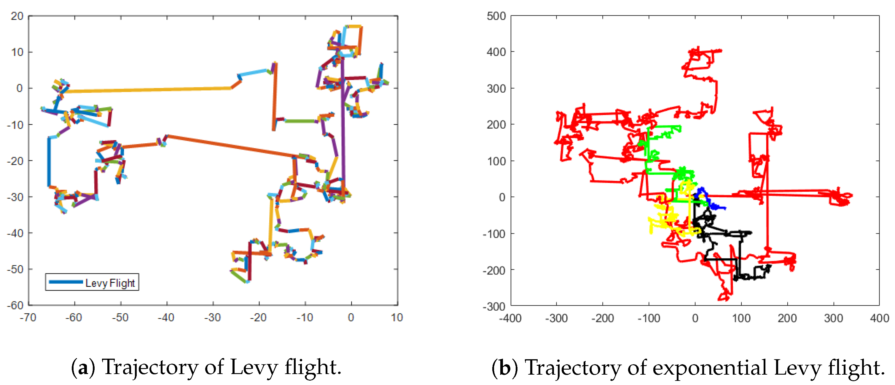
Figure 4a simulates the position update of an individual performing 500 Levy flight. The figure shows that many small-step random wandering and a small number of large-step-skipping behaviors characterize Levy flight [44,45,46]. This unique action pattern makes Levy flight highly stochastic. Thus, it is widely used to improve the algorithm’s ability to jump out of the local optimal solution and enhance global exploration ability. Researchers have also made micro-improvements to Levy flight based on their needs in recent years.
Su et al. [47] and Wang et al. [48] addressed the defect of fixed step size in Levy flight that weakens the accuracy of the algorithm in the later stages of the search. The Cauchy function was adopted to control the step size of the Levy flight. Therefore, the step size of the Levy flight is gradually reduced from a large step size in the early stage of the search to a small step size in the later stages in order to achieve a smooth transition. Wei et al. [49] considered that the value of σ affects the direction and step size of Levy flight. Therefore, adaptive Levy flight is presented to control the position update during the iteration process.
The above researchers embed the improved Levy flight into the iterative formulation of the algorithm and perform a Levy flight perturbation during each iteration to help the algorithm jump out of the local optimal solution. However, the behavior of large step size jumps also weakens the algorithm’s accuracy in finding the optimum and convergence speed in the later stages of the search. If the step size is reduced, the advantage of Levy flight will no longer exist. Given the above limitations, this study adopts the population aggregation degree to implement the Levy flight perturbation strategy. It can fully use the advantages of Levy flight and avoid the impact on optimization accuracy and convergence speed in the later stages of iteration. This study improves the parameters of the Levy flight model to improve its search area such that the perturbed particles can be fully distributed in the search space. The improved parameters are as follows:
σ = Γ ( 1 + β ) × exp ( π β 2 ) Γ 1 + β 2 × β × 2 β 1 2 1 β .
The flight trajectories of the proposed exponential Levy flight and other Levy flight variants are plotted in Figure 4b. From the figure, it can be seen that the exponential-based Levy flight has a more robust search capability than other variants, which is more helpful for the particles caught in precocity to break free from the local optimal solution and redistribute in the search space to continue to search for the optimal solution. The framework of the diversity variation operation is as follows:
1.
Set the population aggregation threshold d.
2.
Calculate the degree of population aggregation σ v a r .
3.
Judge whether σ v a r is less than the threshold d. If less, execute step 4; otherwise, jump to step 2.
4.
Randomly selected 1 / 4 population particles for exponential Levy flight.

2.2.4. The Framework of the MIPOA

The improvement strategy is introduced into POA, and the pseudo-code of the proposed MIPOA algorithm is shown in Algorithm 2:
Algorithm 2 Pseudo-code of MIPOA
Input: 
N , n , T , w max , I , β , p , q
1:
Initialization for pelican populations using Equation (1)
2:
Calculate the fitness value of each pelican particle
3:
while  ( t < T )  do
4:
    Generate the position of the prey at random
5:
    for  i = 1 : N  do
6:
        Exploration phase: Moving towards prey
7:
        for  j = 1 : n  do
8:
           Calculate new status of the jth dimension using Equations (5) and (10)
9:
        end for
10:
        Update the i-th population member using Equation (6)
11:
        Exploitation phase: Hunting is based on the Hardy-Weinberg principle
12:
        for  j = 1 : n  do
13:
           Calculate new status of the j-th dimension using Equation (13)
14:
        end for
15:
        Update the i-th population member using Equation (8)
16:
        Diversity Variation perturbation:
17:
        Calculate the degree of population aggregation σ v a r using Equation (14)
18:
        if  σ v a r < d  then
19:
           Random selection of 1 / 4 pelican population particles for exponential Levy flight
20:
        else
21:
           Recalculate the value of σ v a r until the condition is satisfied
22:
        end if
23:
    end for
24:
end while
Output: 
X b e s t ( X b e s t is the current optimal solution)

3. Low-Illumination Forest Canopy Image Enhancement Based on the MIPOA

3.1. Data Sources and Analysis

Forest canopy images were obtained from the Liangshui Experimental Forestry Farm of the Northeast Forestry University. The Liangshui Experimental Forest is located in Yichun City, Heilongjiang Province (128°47′8″–128°57′19″ E, 47°6′49″–47°16′10″ N), with an east–west width of 13.0 km and a north–south length of 17.0 km, with a total area of 12,133,000 hm2. The Liangshui Experimental Forest is a mixed coniferous and broadleaf forest. The tree species mainly included red pine, spruce, maple, birch, and larch. Canopy images were randomly acquired with a Panasonic DMC-LX5 camera with a fisheye lens Samyang AE 8/3.5 Aspherical IF MC Fisheye with a resolution of 2736 × 2736 in the morning, midday, and evening from July to October. With the wide field of view of the fisheye lens, the resulting hemispherical images of the forest canopy can cover a full range of zenith angles and, therefore, contain rich information about the forest canopy. Forest canopy parameters have been widely used as visual judgment indices for community appearance in forest ecosystem research [50,51]. With the rapid development of image processing technology, obtaining forest canopy parameters and analyzing vegetation growth status and trends using canopy images have become hot research topics. However, the quality of the captured images was poor owing to the influence of the shooting method [52,53], shooting time, light intensity [54], and forest gap [55]. These low-quality canopy images significantly hindered the acquisition of canopy parameters and were not conducive to the subsequent processing of images.
To verify the applicability of the proposed method. Twelve canopy images taken at three different light intensities were selected for testing. The test images are shown in Figure 5. L1–L4 are canopy images acquired under low-illumination conditions. The overall tone is dark, especially at the lower part of the trunk, which is almost mixed with the background and difficult to distinguish. N1–N4 are the canopy images acquired under normal illumination conditions, subject to the way of acquiring canopy images (elevation shot) and the influence of forest gaps. Under ideal lighting conditions, the lower part of the trunk will also appear with low brightness and unclear details. S1–S4 are the canopy images acquired under strong light. They are characterized by uneven brightness, low brightness in the trunks, and blurring of the treetops bordering the sky because of sunlight reflection. Therefore, regardless of the type of canopy image, effective enhancement is an important test for the algorithm.

3.2. IBF

IBF contains four typical grayscale transformation functions, and different transformation functions can enhance different image types [56,57,58]. Figure 6 shows graphs of the four grayscale transformation functions. The horizontal axis represents the gray value of the input image, and the vertical axis represents the gray value of the output image. In this case, Figure 6a is used to expand the darker region, Figure 6b is used to expand the brighter region, Figure 6c is suitable for stretching the middle area, and Figure 6d shows the stretching of the ends and compression of the middle region. The normalization can be described as follows:
F ( u ) = B 1 ( α , β ) 0 u t α 1 ( 1 t ) β 1 d t
B ( α , β ) = 0 1 t α 1 ( 1 t ) β 1 d t .
From (21), different types of nonlinear transformation curves can be obtained by adjusting the parameters α , β . Intelligent algorithms can perform efficient operations in parallel in a complex parameter space to obtain the highest-quality solution possible with minimal problem information and operation costs. The process of finding the IBF parameters is regarded an optimization problem. Using the global optimization search capability of the intelligent optimization algorithm, the values of the optimal transformation parameters α and β can be determined dynamically, thus achieving adaptive enhancement.
The design of the objective function is an essential step in the optimization process. Variance is often used to objectively evaluate the contrast enhancement of an image. The larger its value, the greater the content of the image and the larger the dynamic range of the image pixel values. In this study, IBF was used to enhance the image contrast. Therefore, the selection of the objective function was based on the variance of the image. Specifically, this was calculated as shown in Equation (22):
F = 1 M N x = 1 M y = 1 N i x y 2 1 M N x = 1 M y = 1 N i x y 2 .
Since the intelligent algorithm is used to find the minimum value, the search for the maximum value is changed to the search for the minimum value:
f i t n e s s = F .

3.3. Segmented Gamma Function

Brightness enhancement plays a decisive role in the enhancement of low-illumination images. This can improve the visual effect and quality of the images. The gamma correction function is a classical image brightness enhancement method [59], which is a nonlinear image transformation using the parameter to change the distribution of the image’s brightness. The gamma correction function is, in its basic form, as shown in (24):
T ( l ) = l max l l max γ
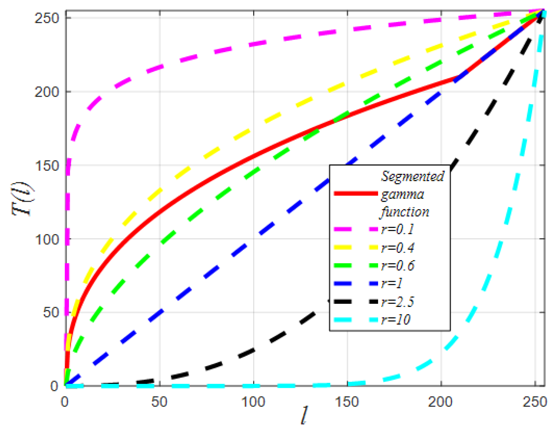
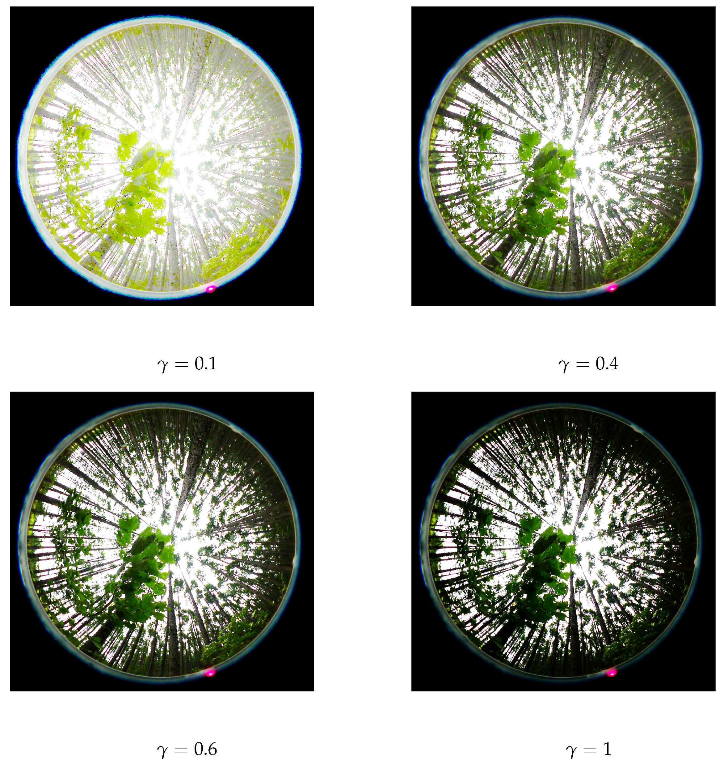
where l is the actual intensity value of the input image, which takes the range of l 0 , l max ; l max is the maximum intensity value of the input image. T ( l ) is the intensity value of the output image after the gamma correction. γ is the correction parameter. When γ is less than 1, the image is stretched to increase its brightness; when γ is greater than 1, it is compressed to darken its brightness. In Figure 7, the dotted lines show the enhancement curves for different γ values. Figure 8 shows the enhancement results of low-illumination forest canopy images with different γ values.
From Figure 8, the processed image is severely exposed when γ = 0.1 . There is no change in the brightness of the enhanced image when γ = 1 . The processed image has a better quality when γ is 0.4 and 0.6. The brightness is superior at γ = 0.4 , but the processing of the sky portion is unsatisfactory, and the treetop bordering the sky is blurred due to the exposure. The inferiority of the brightness is obvious at γ = 0.6 , although the detail of the sky portion is superior to that at γ = 0.4 . In enhancing the low-illumination canopy image, there is a contradiction between the brightness enhancement of the dark areas and the exposure of the high-brightness areas. This contradiction stems from the fact that gamma is a global enhancement method. During the image brightness stretching, regardless of the value of γ , the bright area will stretch the image. If the brightness of the dark area is moderate, the bright area will inevitably appear in the exposure phenomenon. If the brightness of the highlighted area is mild, the brightness enhancement of the dark area is not noticeable, and the details cannot be emphasized. For this defect, the gamma correction function is improved as follows:
T ( l ) = k l max l l max γ , l a l , l > a
k = a l max a l max γ
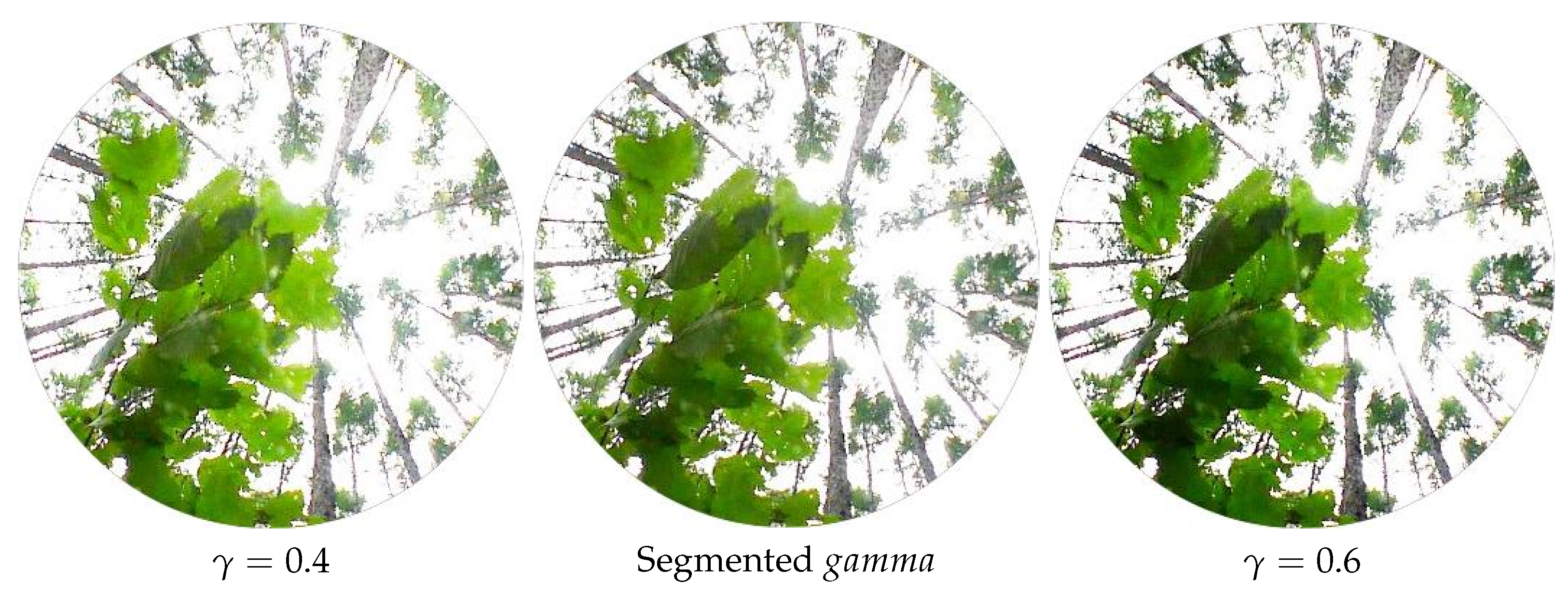
where γ is the luminance correction factor. The histogram of the same type of canopy image is very similar, and γ = 0.4 in this study. a is the input image intensity threshold—in this study, a = 210 . The improved gamma correction function is segmented from (25). The coefficient k is added to the gamma correction function when l a. The increase of coefficient k causes the output T ( l ) value of the gamma correction function to be located between γ = 0.4 and γ = 0.6 in the low-brightness region ( l < 150 ) . The image of the dark-region was in the optimal brightness-stretching interval. The stretching intensity is reduced in the moderate brightness region ( 150 < l < 210 ) , and its output T ( l ) value is less than that of γ = 0.6 to prevent overstretching. In the highlighted area ( 210 < l < 255 ) , the output T ( l ) value is equal to that of γ = 1 , indicating that the brightness of the highlighted area is not enhanced. This improvement prevents overexposure of the highlighted areas and effectively preserves the details. The segmented gamma correction function curves are shown as solid red lines in Figure 7. Figure 9 shows the enhancement results of the sky area at γ = 0.4 , segmented gamma, and γ = 0.6 , respectively. As can be seen from the figure, the brightness of the sky region enhanced by the segmented gamma correction function is better than that of the enhancement result at time γ = 0.6 , and the details of the border between the treetops and the sky are better than in the enhancement result at time γ = 0.4 . The results are shown in Figure 9. The segmented gamma correction function improves the brightness of the image and prevents overexposure of the sky area.

3.4. Algorithm Implementation

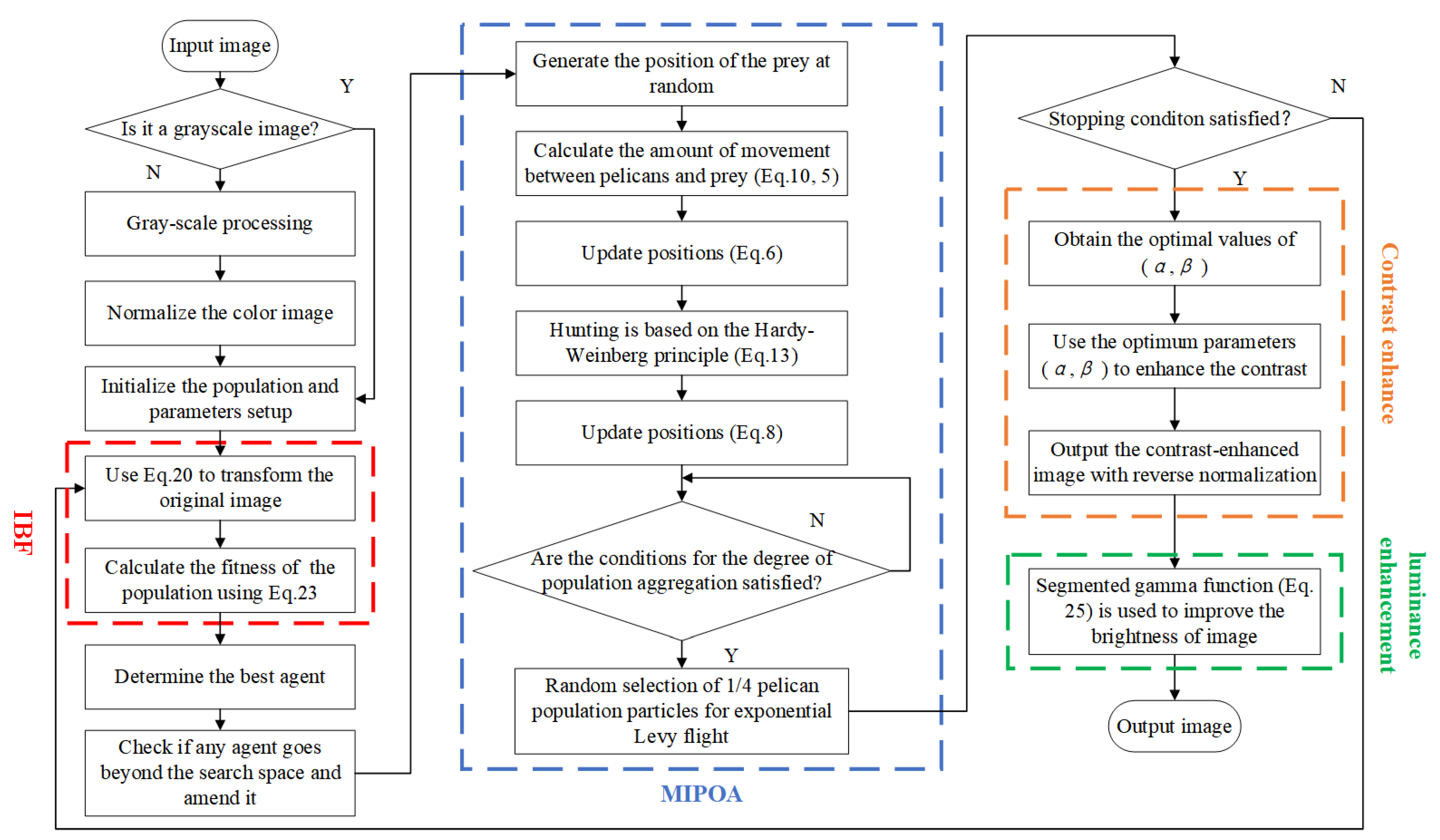
In this study, we enhanced the low-illumination forest canopy image in terms of contrast and brightness. First, MIPOA searches for the optimal parameters ( α , β ) of IBF to enhance contrast. It is worth noting that the proposed MIPOA can find the optimum, reducing the possibility of falling into the local optimum in the IBF parameter search. Thus, the contrast of the image is effectively improved. Second, the segmented gamma correction function is designed to equalize the brightness of the low-illumination canopy image. Figure 10 shows the flowchart of the proposed MIPOA-based enhancement algorithm. The framework of the proposed algorithm is as follows:
1.
Input the image to be enhanced.
2.
Judge whether the input image is a grayscale image. If this is true, then normalization is performed directly. If it is a color image, then grayscale processing is performed first followed by normalization.
3.
Generate the population and parameters of MIPOA.
4.
Apply (20) to achieve image contrast enhancement.
5.
Calculate the fitness value of the population using (23).
6.
Update the best agent.
7.
Check whether the agent goes beyond the search space.
8.
Generate the position of the prey at random.
9.
Calculate the amount of movement between the pelicans and prey ( 10 , 5 ) .
10.
Update new positions (6).
11.
Perform hunting based on the Hardy–Weinberg principle (13).
12.
Update new positions (8).
13.
Determine whether the aggregation of populations satisfies these requirements.
14.
If the conditions are met, perform random selection of 1 / 4 pelican population particles for exponential Levy flight.
15.
Repeat Steps 3–14 until the algorithm meets the stop condition.
16.
Output the result of MIPOA as the optimal values of ( α , β ) for IBF.
17.
Use the optimum parameters ( α , β ) found in Step 16 to enhance the contrast of the input image.
18.
Output the contrast-enhanced image with reverse normalization.
19.
Use the segmented gamma function to improve the brightness of the image (25).
20.
Output the enhanced image.

4. Performance Testing and Analysis of the MIPOA

4.1. Benchmark Test Functions

As shown in Table 2, six benchmark functions were selected for testing to verify the performance of the MIPOA. Among them, F 1 F 2 are high-dimensional, single-peak functions. Such functions have only one global optimum and no local optimum. They were used to test the optimization speed and exploitation capability of the algorithms. F 3 F 4 are high-dimensional, multi-peak functions. These functions have multiple local optimal values, and many local optimal values will increase the probability of the algorithm falling into the local optimal solution. Therefore, this type of function is suitable for testing the algorithm’s exploration ability and the ability to jump out of the local optimal solution. F 5 F 6 are low-dimensional, multi-peak functions. Compared with the high-dimensional, multi-peak function, its dimension is a lower fixed dimension. This type of function is used to test the balance ability between algorithm exploration and exploitation.

4.2. Experimental Setup

The experiment was conducted on an Intel [email protected] GHz PC with 16 GB of RAM and Windows 11. To objectively evaluate the performance of the MIPOA, the basic POA and five POA variants (IPOA1 [28], IPOA2 [29], IPOA3 [30], IPOA4 [31], and IPOA5 [32]) were selected for the comparative algorithm. In the experiment, the population size ( N ) was set to 30, and the maximum number of iterations ( T ) was set to 500. Each benchmark function was run independently 30 times to avoid the possibility of chance errors in the optimization search.

4.3. Comparative Results and Analysis of the MIPOA with POA Variants

4.3.1. Effect of the Value of the Threshold Parameter redd on the Performance of the Algorithm

The threshold parameter d needs to be decided according to the specific problem. If the threshold is too high, the algorithm cannot jump out of the local optimal solution in time; if the threshold is too low, the individuals in the population will be perturbed frequently, affecting the population’s optimization accuracy and convergence speed. In this study, Table 2 is used as the test function, and the mean fitness value is used as the evaluation index to conduct 30 trials to select the optimal threshold parameter d. The experimental results are shown in Table 3. Table 3 shows that in optimizing F 1 and F 2 , the highest optimization accuracy is achieved at d = 0.5 , while d = 0.7 and d = 0.3 have the highest search accuracy on F 3 and F 4 , respectively. d = 0.5 is slightly lower and ranks second. From the optimization results of F 5 and F 6 , it can be seen that the value of d does not affect them, which confirms that the exponential Levy flight perturbation strategy based on population variation does not affect the balance between algorithm exploration and exploitation.
In summary, d = 0.5 is selected as the final threshold value in this study. In addition, scholars often use a random number, r a n d , for threshold selection. However, in this test, it is far inferior to other fixed thresholds.

4.3.2. Optimization Accuracy Analysis

The mean value reflects the algorithm’s optimization accuracy. The closer the mean value is to the optimal value of the function, the higher the accuracy of the optimization search [60,61,62]. The mean fitness value of each algorithm on the test function is shown in Table 4. From Table 4, it can be seen that on F 1 , IPOA1∼IPOA5 are inferior to the basic POA. On F 2 , IPOA1 and IPOA5 are slightly better than the POA but are far from the optimal value. In contrast, the MIPOA outperforms the other variants by 17 orders of magnitude on F 1 and achieves the ideal value on F 2 . It shows strong exploitation ability and the ability to jump out of the local optimal solution. MIPOA has the same obvious advantage on F 3 and F 4 , and the searching accuracy is 100 % better than the comparison algorithms, which have strong exploration ability. In addition, the IPOA1 and IPOA5 are also effective in improving the exploration ability, with better search accuracy than the POA. Only the MIPOA obtains the ideal value for F 5 and F 6 , outperforming the other POA variant algorithms. This shows that the MIPOA can improve the exploitation and exploration capabilities while striking a balance between the two.

4.3.3. Stability Analysis

Table 5 shows the standard deviation values of each algorithm on the test function. The lower the standard deviation value, the better the stability [63,64,65]. From Table 5, it is clear that the MIPOA achieves all the optimal values and outperforms the comparison algorithm by 100 % in terms of stability. The five POA variant algorithms have their own merits regarding stability. Compared to the POA, the IPOA1 IPOA5 algorithms improved instability by 66.67 % , 50 % , 100 % , 50 % , and 83.33 % , respectively. Among them, IPOA3 performs well and garners an overall improvement in stability, but its improvement is low. MIPOA algorithm improves by 16 , 29 , 28 , 6 , and 4 orders of magnitude relative to the IPOA3 on F 1 , F 3 F 6 , respectively. The MIPOA achieves the desired value of 0 on F 2 and only 0.1496 for IPOA3, which is a far cry from the others.

4.3.4. Convergence Analysis

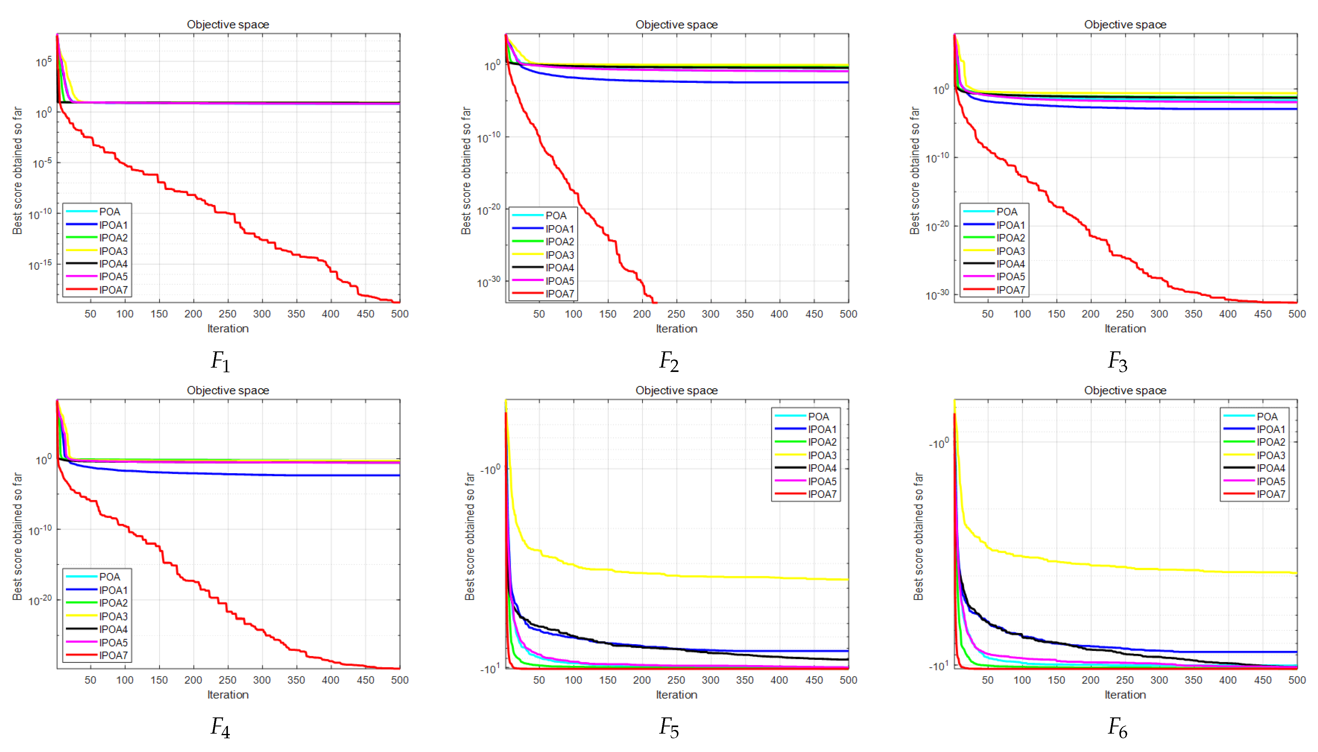
The convergence curve can visualize the convergence speed, convergence accuracy, and ability to jump out of the local optimal solution of each algorithm [66,67,68]. Figure 11 shows the convergence curves of the test functions. The figure shows that the MIPOA algorithm’s optimization accuracy is significantly better than other algorithms on F 1 F 4 . When other algorithms are trapped in the local optimal solution and cannot break free, the MIPOA can successfully break through the constraints of the local optimal solution to continue to find the overall optimum. Additionally, the convergence curve steadily progresses, which indicates that it has strong stability. There is not much difference in the optimization accuracy of the algorithms for F 5 and F 6 , and the MIPOA is slightly better than the comparison algorithms in terms of optimization accuracy and convergence speed. On the contrary, IPOA3 is somewhat lower. It is consistent with the results of the data in Table 4.

4.3.5. Statistical Analysis

The Wilcoxon rank sum test is a non-parametric statistical method. Compared with common tests such as the t-distribution test, Fisher’s eExact test, and the Kruskal–Wallis H test, the Wilcoxon rank sum test has the following advantages:
(1)
The distribution is free, and assuming that the sample data follows a normal distribution is unnecessary.
(2)
Strong stability; not affected by outliers.
(3)
Simple, convenient, intuitive, and understandable.
Therefore, the non-parametric Wilcoxon rank–sum test is used to evaluate algorithms’ performance and statistically verify whether there are significant differences in the results of each run between algorithms [69,70,71].
Where 0.05 is the significance level, a p-value greater than 0.05 means that the difference between the two groups is insignificant, and a p-value less than 0.05 means that the difference between the two groups is substantial. The Wilcoxon rand rank–sum test values for each algorithm are shown in Table 6. The MIPOA is statistically different from all the comparative algorithms, indicating that the MIPOA has improved significantly in statistical analysis.

5. Results and Discussion of MIPOA-Based Enhancement Algorithm

5.1. Evaluation Indicators

5.1.1. FSIM

FSIM compares the feature similarity between the original image and the enhanced image. The larger the value of FSIM, the more similar the original image is to the enhanced image and the higher the quality of the enhanced image [72]. The formula for FSIM is shown in Equation (27).
F S I M = x Ω S L ( x ) × P C m ( x ) x Ω P C m ( x )
where Ω is the pixel value of the whole image, S L ( x ) denotes the similarity value, and P C m ( x ) represents the phase consistency measure.
P C m = max P C 1 ( x ) , P C 2 ( x ) .
P C 1 ( x ) and P C 2 ( x ) denote the phase coherence of the reference and enhanced images, respectively.
S L ( x ) = S P C ( x ) α · S G ( x ) β
S P C ( x ) = 2 P C 1 ( x ) × P C 2 ( x ) + T 1 P C 1 2 ( x ) × P C 2 2 ( x ) + T
S G ( x ) = 2 G 1 ( x ) × G 2 ( x ) + T 2 G 1 2 ( x ) × G 2 2 ( x ) + T 2
where S P C ( x ) represents the feature similarity of the image; S G ( x ) represents the gradient similarity of the image; G 1 ( x ) and G 2 ( x ) represent the gradient magnitude of the reference image and the enhanced image, respectively; and α , β , T 1 and T 2 are constants.

5.1.2. Entropy

Entropy measures the richness of the information contained in an image. The greater the entropy value of an image, the greater the amount of information contained in the image and the richer the details [57]. The calculation formula is given by Equation (32).
H = i = 0 255 p ( i ) × log 2 ( p ( i ) )
where p ( i ) denotes the probability of gray value i.

5.1.3. CII

The CII is a classic metric used to evaluate the effect of contrast improvement in images [73]. It quantifies the degree of contrast enhancement in an image to judge the impact of contrast improvement [74]. The higher the value of CII, the more significant the contrast improvement. The calculation formula is shown in (33).
CII = s t d I e n h a n c e d s t d I o r i g i n a l m e a n I e n h a n c e d m e a n I o r i g i n a l
I o r i g i n a l is the original image, I e n h a n c e d is the processed image, std(.) is the standard deviation, and mean(.) is the mean.

5.1.4. Average Gradient

The average gradient can be sensitive to the image’s ability to express the contrast of small details. Therefore, it is often used as a measure of image clarity. Usually, the more significant the average gradient value, the greater the rate of change of gray levels in a specific image direction, the richer the layers, and the better the visual effect presented by the image [75]. The expression defining the average gradient is
A G = 1 m × n i = 1 m j = 1 n f x 2 + f y 2 / 2 1 / 2
where m and n are the width and height of the image, respectively; f / x represents the horizontal gradient; and f / y represents the vertical gradient.

5.1.5. Pixel Mean

The pixel mean reflects a color image’s brightness, exposure, and contrast better than the gray mean. A higher pixel mean value indicates that the image is brighter overall, with sharper and more precise details. A lower pixel mean value indicates a darker image with less detail. However, a higher pixel mean is not always better. An overexposed image has a high pixel mean. The expression for pixel mean value is given below:
M e a n = 1 m n i = 1 m j = 1 n P i , j
where m and n are the width and height of the image, respectively, and P i , j is the pixel value corresponding to the ( i , j ) position.

5.2. Analysis of IBF Parameter Optimization Experiment Results

To verify the effectiveness of MIPOA in determining the optimal IBF parameters, HWOA [25], FAG [26], PSO [22], ChOA [21], and POA were used for comparison experiments. Twelve typical low-illumination canopy images (Figure 5) were selected as the experimental images. FSIM, entropy, and CII were used as evaluation indices for the merit of enhancement.
The FSIM values obtained by each intelligent algorithm for the forest canopy images are listed in Table 7. From the table, it is clear that the MIPOA obtained competitive results for all types of canopy images. The optimal FSIM values were obtained for nine canopy images, which were slightly lower than those of the PSO, HWOA, and PSO algorithms on L2, N4, and S4, and are located in the second position. This indicates that the enhanced image based on the MIPOA algorithm has a higher feature similarity with the original image, less distortion, and more natural enhancement. The ChOA algorithm is also tied with the MIPOA algorithm for first place on seven images, but it is better at enhancing canopy images with normal illumination. Although the PSO algorithm obtained the optimal FSIM values on L2 and S2, it had much lower FSIM values on the other images than the other algorithms and was less stable. The HWOA outperformed the comparison algorithm for N4. However, the FSIM values obtained on other images are as good as those of FAG and POA, better than PSO and inferior to ChOA and MIPOA.
The entropy values obtained by each intelligent algorithm on the canopy images are shown in Table 8. The table shows that the MIPOA algorithm performs well on low-illumination (L1–L4) and normal-illumination (N1–N4) canopy images, outperforming the comparison algorithms by 75%. For instance, the entropy values of PSO, ChOA, FAG, HWOA, POA, and MIPOA are 0.7238, 0.7238, 0.7238, 0.7238, 0.7238, 0.7238, 0.7238, and 1.2062, respectively, at enhanced L3. This indicates that the comparison algorithms have fallen into the local optimal solution and have not found the optimal parameter of IBF. Therefore, the FSIM values of the comparison algorithms are the same. At the same time, the MIPOA algorithm can break free from the local optimal solution and continue to find the overall optimal parameter. The obtained entropy value is higher, and the enhanced image has richer details and higher image quality. In the enhancement of N1, the entropy value of all algorithms is 0.7525, indicating that all algorithms have the same performance in terms of optimization seeking on N1, and the enhanced image contains the same degree of information richness.
Table 9 shows the CII values obtained by each intelligent algorithm for the canopy image. Owing to the limitations of the shooting method for forest canopy images, regardless of the illumination level under which the canopy image is acquired, there will be low brightness and hidden details in the tree trunks. Simultaneously, strong light makes sky areas susceptible to losing more information. Therefore, enhancing the image contrast is particularly important so that details can be highlighted. As shown in Table 9, the MIPOA algorithm has clear advantages. In particular, when dealing with normal-illumination canopy images, all optimal CII values were obtained. The MIPOA algorithm outperformed the comparison algorithm by 75 % on low-light canopy images and was inferior to the ChOA only for L2. On strong-light canopy images, the MIPOA algorithm performed mediocrely and outperformed the comparison algorithm only on S1 and S3. It was inferior to PSO for S2 and to ChOA for S4. The MIPOA algorithm obtained nine optimal CII values and three suboptimal values for 12 canopy images. This shows that the enhanced images based on the MIPOA algorithm have better contrast enhancement and stronger stability. In contrast, PSO and the ChOA are not sufficiently stable. The PSO algorithm has a CII value of 0.81039 on S2, which is better than the other algorithms, but the CII values of 0.13413 , 0.18988 , and 0.13844 for L 1 , N 3 , and S4, respectively, are lower than those of the other algorithms. ChOA achieved the worst value at S3. FAG, HWOA, and POA performed poorly in obtaining CII values and did not obtain optimal values.
In general, through the above analysis, the performance indexes obtained by each algorithm in the process of optimization of IBF parameters appear to have many equal data, which is because the image is a forest canopy image, the trees are intricate and complex, the branches and leaves are crisscrossed, and the light has a great impact on the image quality. For intelligent algorithms, the challenge is very difficult. If the intelligent algorithms seek optimization with low accuracy, it is very easy to fall into the local optimum, and the enhancement fails. L3 is the best example. Only the MIPOA algorithm breaks through the constraints of the local optimal solution and finds the optimal parameters of the IBF. The MIPOA algorithm performs well; out of 36 data sets, the MIPOA algorithm obtains the optimal value of 25, and 11 is located in second place. It shows strong stability. In addition, MIPOA is inferior to POA only on L2 images, and is 91.67% better than POA across all other images, which proves the necessity of improving the POA algorithm.

5.3. Experimental Results and Analysis of Low-Illumination Forest Canopy Images

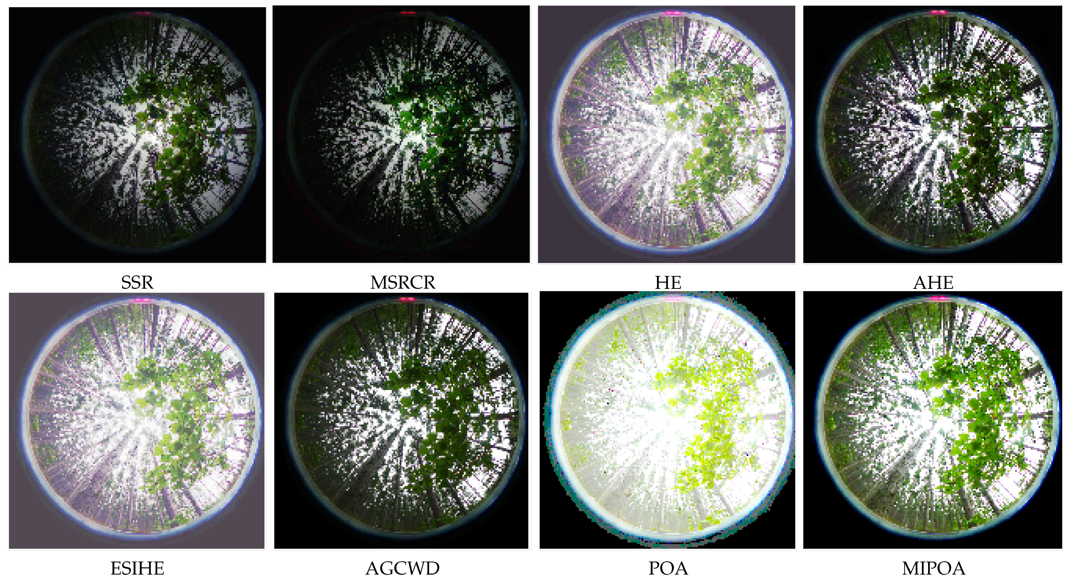
In this test, the segmented gamma function is added to the IBF to enhance the image brightness, constituting a complete low-illumination forest canopy image enhancement method based on the MIPOA algorithm. To verify the accuracy and effectiveness of the proposed method in low-illumination forest canopy image enhancement, traditional enhancement methods such as SSR, MSRCR, HE, AHE, ESIHE, AGCWD, and POA were used as comparison algorithms. Subjective and objective evaluation metrics were used to assess the enhanced image improvement effect.

5.3.1. Subjective Evaluation Analysis

Due to space limitations, this study only showed the enhancement results for canopy L3. The enhancement results for each algorithm for the L3 image are shown in Figure 12. From the figure, the brightness of SSR and the saturation of MSRCR are enhanced in the middle highlighted area. However, the darker trunk portion showed almost no enhancement. The HE and ESIHE methods effectively improved the brightness of the low-illumination canopy image, highlighting the details in darker areas. However, the saturation of the enhanced image was low, and color degradation occurred. The AHE and AGCWD algorithms effectively improved the image contrast, and the difference between the bright and dark parts of the enhanced image was obvious. The details of the images are clear. However, this method lacks brightness enhancements. The enhancement results based on the POA are poor, with serious defects, such as exposure and color distortion. This stems from the weak optimization accuracy of the POA algorithm, which does not find the optimal parameters for the contrast enhancement of the image when optimizing the IBF parameters. The enhancement results based on MIPOA have obvious advantages and significantly improve the contour details in low-illumination regions. The highlighted areas in the sky are not overexposed because of the enhancement of dark places, and the details are preserved. In addition, the overall tone is more realistic and the colors are more vivid, saturated, and without color distortion.

5.3.2. Objective Evaluation Analysis

Table 10 lists the pixel mean values obtained using each enhancement algorithm. It is clear from the table that the pixel mean values of ESIHE and HE are higher than those of the other algorithms, are located between [ 129.6689 , 150.8542 ] , and have higher brightness. However, both ESIHE and HE are global-enhancement algorithms. For forest canopy images, if no special treatment is applied to the bright areas, the bright regions are bound to be over enhanced if the pixel mean value after enhancement is too high. This is best demonstrated by the enhancement results of ESIHE and HE in Figure 12. The pixel mean values of AHE and AGCWD were similar and were all in the range of [ 59.4392 , 87.7792 ] . This indicates that their enhanced images have low brightness and cannot be effectively enhanced. The pixel mean values of SSR and MSRCR were between [ 0.11069 , 0.25879 ] , which were much lower than those of the other algorithms. This indicates that the enhanced image has almost no change and the enhancement fails. Canopy images enhanced based on the POA algorithm are volatile in terms of pixel mean value, and the pixel mean value is approximately 110 on L2, L4, and S1–S4, which is visually better for low-illumination canopy images. However, the pixel average is higher on L3 and N1–N4 and even reaches 188.433 on N1, which is in a severe exposure state. This is due to the poor stability of the POA algorithm and the failure of the enhancement of individual images. The MIPOA algorithm, on the other hand, has strong optimization accuracy and good stability. Better pixel averages were obtained for each test image. There was no excessive fluctuation, moderate brightness, or good visual effect.
Table 11 presents the average gradient values obtained using each enhancement algorithm. As shown in Table 11, the MIPOA-based enhancement algorithm has clear advantages. This is better than other contrast algorithms, especially in N2 and N4 images, which are canopy images with complex backgrounds, intricate forest trees, and small branches and leaves hidden in a dark background that cannot be distinguished. The successful improvement in the contrast of the N2 and N4 images illustrates the effectiveness of MIPOA in contrast enhancement. In addition, the AHE algorithm achieved good results in terms of contrast improvement, slightly lower than MIPOA, and ranked second. The POA competes strongly for enhancing the L2, S2, and S3 images; however, its stability needs to be improved. It outperformed the SSR and MSRCR algorithms only for L3 and N1, respectively. The average gradient values obtained by the SSR and MSRCR algorithms were between 0.17349 and 0.30519, which were much lower than those obtained by the other algorithms. This indicates that their enhanced images showed almost no improvement in contrast, making them unsuitable for enhancing the contrast of the forest canopy images.

6. Conclusions and Outlook

In summary, each enhancement algorithm’s subjective and objective evaluations show that the enhancement method based on the MIPOA proposed in this study achieves better results in enhancing low-illumination forest canopy images. It effectively improves the image brightness and contrast and the defects of low brightness and unclear image details in low-illumination forest canopy images. The details of the dark areas in the enhanced image are prominent, and the details of the bright regions are preserved. The visual colors are bright and vivid.
  • The nonlinear decreasing coefficient, Hardy–Weinberg theorem, and diversity variant operation are incorporated into the POA mathematical model to further enhance the algorithm’s ability to explore, exploit, and escape local optimal solutions. The experimental results of the benchmarking function demonstrate that the performance of MIPOA is comprehensively improved and surpasses the five POA variant algorithms in terms of optimization search accuracy, stability, convergence, and statistical analysis.
  • IBF is an effective method for improving the contrast of an image; however, its parameters require manual configuration, and parameter selection is inefficient. In IBF parameter optimization, the MIPOA outperforms PSO, ChOA, FAG, HWOA, and POA in FSIM, entropy, and CII. This indicates that the MIPOA algorithm improves the optimization accuracy of the IBF parameters such that the enhanced canopy image exhibits less distortion, contains rich information, and demonstrates effectively enhanced contrast.
  • Based on the characteristics of low brightness and uneven distribution of forest canopy images, a segmented gamma correction function was designed to increase the brightness of dark areas while avoiding over-enhancement of the bright regions. In low-light forest canopy image enhancement, the MIPOA-based enhancement method achieves moderate pixel averages and high average gradients, which are superior to those of six traditional image enhancement methods: SSR, MSRCR, HE, AHE, ESIHE, and AGCWD.
  • Nevertheless, this study has certain limitations. To prevent overexposure of the bright regions, the segmented gamma correction function does not perform any processing on the bright areas. This preserved the brightness of the bright regions. In the event that the image is exposed and conceals its details, the processing effect of the proposed method, although superior to traditional enhancement algorithms, is not as effective as that of the canopy image with low and normal illumination. Therefore, further development of the segmented gamma correction function is necessary to expose the high-brightness areas. Additionally, the MIPOA algorithm demonstrates strong superiority in the benchmark function, which can be applied to practical engineering problems, such as structural optimization.

Author Contributions

X.Z. and L.Z. contributed to the idea of this paper; X.Z. performed the experiments; J.W. and A.M.E.M. analyzed data; X.Z. wrote the manuscript; X.Z. and L.Z. contributed to the revision of this study. All authors have read and agreed to the published version of the manuscript.

Funding

This research was funded by the Fundamental National Key R&D Program of China under Grant 2021YFC2202502, the Fundamental Research Funds for the Central Universities under Grant (No. 2572023CT15), the National Natural Science Foundation of China (No. 31370710), and the Postdoctoral Research Foundation of Heilongjiang Province (No. LBH-Q13007).

Informed Consent Statement

This article does not contain studies with human participants or animals. Statement of informed consent is not applicable since the manuscript does not contain any patient data.

Data Availability Statement

The data used to support the findings of this study are available from https://pan.baidu.com/s/1CAi_L9P-s4p_VonwPb9cKw?pwd=c395 (accessed on 2 September 2024), password: c395.

Acknowledgments

The authors thank the anonymous reviewers for their useful comments that improved the quality of the paper.

Conflicts of Interest

The authors declare no conflicts of interest.

References

  1. Woldamanuel, E.M. Grayscale Image Enhancement Using Water Cycle Algorithm. IEEE Access 2023, 11, 86575–86596. [Google Scholar] [CrossRef]
  2. Sengupta, D.; Biswas, A.; Gupta, P. Non-linear weight adjustment in adaptive gamma correction for image contrast enhancement. Multimed. Tools Appl. 2021, 80, 3835–3862. [Google Scholar] [CrossRef]
  3. Prakash, A.; Bhandari, A.K. Cuckoo search constrained gamma masking for MRI image contrast enhancement. Multimed. Tools Appl. 2023, 82, 40129–40148. [Google Scholar] [CrossRef]
  4. Asiri, A.A.; Soomro, T.A.; Shah, A.A.; Pogrebna, G.; Irfan, M.; Alqahtani, S. Optimized Brain Tumor Detection: A Dual-Module Approach for MRI Image Enhancement and Tumor Classification. IEEE Access 2024, 12, 42868–42887. [Google Scholar] [CrossRef]
  5. Mishra, A.K.; Choudhry, M.S.; Kumar, M. Underwater image enhancement using multiscale decomposition and gamma correction. Multimed. Tools Appl. 2023, 82, 15715–15733. [Google Scholar] [CrossRef]
  6. Zhang, W.; Zhuang, P.; Sun, H.H.; Li, G.; Kwong, S.; Li, C. Underwater Image Enhancement via Minimal Color Loss and Locally Adaptive Contrast Enhancement. IEEE Trans. Image Process. 2022, 31, 3997–4010. [Google Scholar] [CrossRef] [PubMed]
  7. Sreeshan, K.; Dinesh, R.; Renji, K. Nondestructive inspection of aerospace composite laminate using thermal image processing. SN Appl. Sci. 2020, 2, 1830. [Google Scholar] [CrossRef]
  8. Bhandari, A.K. A logarithmic law based histogram modification scheme for naturalness image contrast enhancement. J. Ambient Intell. Humaniz. Comput. 2020, 11, 1605–1627. [Google Scholar] [CrossRef]
  9. Stark, J.A. Adaptive image contrast enhancement using generalizations of histogram equalization. IEEE Trans. Image Process. 2000, 9, 889–896. [Google Scholar] [CrossRef]
  10. Pizer, S.M.; Amburn, E.P.; Austin, J.D.; Cromartie, R.; Geselowitz, A.; Greer, T.; ter Haar Romeny, B.; Zimmerman, J.B.; Zuiderveld, K. Adaptive histogram equalization and its variations. Comput. Vision Graph. Image Process. 1987, 39, 355–368. [Google Scholar] [CrossRef]
  11. Liu, J. Research on Low Illumination Image Enhancement Based on Metaheuristic Algorithm; Tongfang Knowledge Network (Beijing) Technology Co., Ltd.: Beijing, China, 2020. [Google Scholar] [CrossRef]
  12. Zuiderveld, K.J. Contrast Limited Adaptive Histogram Equalization. In Graphics Gems; Academic Press: Cambridge, MA, USA, 1994; pp. 474–485. [Google Scholar] [CrossRef]
  13. Huang, S.C.; Cheng, F.C.; Chiu, Y.S. Efficient Contrast Enhancement Using Adaptive Gamma Correction With Weighting Distribution. IEEE Trans. Image Process. 2013, 22, 1032–1041. [Google Scholar] [CrossRef] [PubMed]
  14. Ibrahim, H.; Kong, N.S.P. Brightness Preserving Dynamic Histogram Equalization for Image Contrast Enhancement. IEEE Trans. Consum. Electron. 2007, 53, 1752–1758. [Google Scholar] [CrossRef]
  15. Singh, K.; Kapoor, R. Image enhancement using Exposure based Sub Image Histogram Equalization. Pattern Recognit. Lett. 2014, 36, 10–14. [Google Scholar] [CrossRef]
  16. Senthamarai, G.; Santhi, K. Dynamic multi-histogram equalisation for image contrast enhancement with improved brightness preservation. In Proceedings of the 2015 2nd International Conference on Electronics and Communication Systems (ICECS), Coimbatore, India, 26–27 February 2015; pp. 1205–1209. [Google Scholar] [CrossRef]
  17. Li, C.; Liu, J.; Liu, A.; Wu, Q.; Bi, L. Global and Adaptive Contrast Enhancement for Low Illumination Gray Images. IEEE Access 2019, 7, 163395–163411. [Google Scholar]
  18. Choi, D.H.; Jang, I.H.; Kim, M.H.; Kim, N.C. Color image enhancement using single-scale retinex based on an improved image formation model. In Proceedings of the 2008 16th European Signal Processing Conference, Lausanne, Switzerland, 25–29 August 2008; pp. 7–18. [Google Scholar]
  19. Rahman, Z.; Jobson, D.J.; Woodell, G.A. Multi-scale retinex for color image enhancement. In Proceedings of the ICIP (3), Lausanne, Switzerland, 19 September 1996; pp. 1003–1006. [Google Scholar] [CrossRef]
  20. Jobson, D.J.; Rahman, Z.; Woodell, G.A. A multiscale retinex for bridging the gap between color images and the human observation of scenes. IEEE Trans. Image Process. 1997, 6, 965–976. [Google Scholar] [CrossRef]
  21. Du, N.; Luo, Q.; Du, Y.; Zhou, Y. Color Image Enhancement: A Metaheuristic Chimp Optimization Algorithm. Neural Process. Lett. 2022, 54, 4769–4808. [Google Scholar] [CrossRef]
  22. Qu, X.; Yu, Y.; Bian, S.; Xiao, C. Design of a Contrast Enhancement Algorithm for Visual Communication Images Based on PSO. In Proceedings of the 2023 International Conference on Power, Electrical Engineering, Electronics and Control (PEEEC), Athens, Greece, 25–27 September 2023; pp. 445–449. [Google Scholar] [CrossRef]
  23. Song, W.; Lin, C.B. Improved adaptive image enhancement algorithm based on SSA. In Proceedings of the 2023 IEEE International Conference on Control, Electronics and Computer Technology (ICCECT), Jilin, China, 28–30 April 2023; pp. 54–57. [Google Scholar] [CrossRef]
  24. Asokan, A.; Popescu, D.E.; Anitha, J.; Hemanth, D.J. Algorithm Based Non-linear Contrast Stretching for Satellite Image Enhancement. Geosciences 2020, 10, 78. [Google Scholar] [CrossRef]
  25. Braik, M. Hybrid enhanced whale optimization algorithm for contrast and detail enhancement of color images. Clust. Comput. 2024, 27, 231–267. [Google Scholar] [CrossRef]
  26. Shen, R.; Zhou, M.; Ling, S. Image Enhancement Technology Based on Improved FA Algorithm and Incomplete Beta Function. J. Chongqing Technol. Bus. Univ. Nat. Sci. Ed. 2023, 40, 57–63. [Google Scholar] [CrossRef]
  27. Trojovský, P.; Dehghani, M. Pelican Optimization Algorithm: A Novel Nature-Inspired Algorithm for Engineering Applications. Sensors 2022, 22, 855. [Google Scholar] [CrossRef]
  28. Zhou, J.; Zheng, R.; Hou, H. Improved pelican algorithm for optimizing LSTM based temperature prediction of reheating furnace billets. Foreign Electron. Meas. Technol. 2023, 42, 174–179. [Google Scholar] [CrossRef]
  29. Ye, Y.; Wei, W. Feature selection method based on pelican optimization algorithm integrated with multi-strategies. Microelectron. Comput. 2023, 40, 19–25. [Google Scholar] [CrossRef]
  30. Yang, G.; Hu, H.; Wang, X.; Feng, S.; Wang, F.; Sun, J. Research on Image Matching Method Based on Mass Perturbation Pelican Optimization Algorithm. J. Zhengzhou Univ. Nat. Sci. Ed. 2023, 47, 1–7. [Google Scholar] [CrossRef]
  31. Li, Z.; Zhao, T.; Li, C.; Jie, J.; Shi, H.; Yang, H. Improved Pelican Optimization Algorithm Fused with Multi-Strategy. Control Eng. China 2023, 05, 1–15. [Google Scholar] [CrossRef]
  32. Tuerxun, W.; Xu, C.; Haderbieke, M.; Guo, L.; Cheng, Z. A Wind Turbine Fault Classification Model Using Broad Learning System Optimized by Improved Pelican Optimization Algorithm. Machines 2022, 10, 407. [Google Scholar] [CrossRef]
  33. Igel, C.; Toussaint, M. Recent results on no-free-lunch theorems for optimization. arXiv 2003, arXiv:cs/0303032. [Google Scholar]
  34. Goldberg, D.E.; Holland, J.H. Genetic Algorithms and Machine Learning. Mach. Learn. 1988, 3, 95–99. [Google Scholar] [CrossRef]
  35. Kennedy, J.; Eberhart, R. Particle swarm optimization. In Proceedings of the ICNN’95—International Conference on Neural Networks, Perth, WA, Australia, 27 November–1 December 1995; pp. 1942–1948. [Google Scholar] [CrossRef]
  36. Rao, R.V.; Savsani, V.J.; Vakharia, D.P. Teaching–learning-based optimization: A novel method for constrained mechanical design optimization problems. Comput. Aided Des. 2011, 43, 303–315. [Google Scholar] [CrossRef]
  37. Mirjalili, S.; Mirjalili, S.; Lewis, A. Grey wolf optimizer. Adv. Eng. Softw. 2014, 69, 46–61. [Google Scholar] [CrossRef]
  38. Mirjalili, S.; Lewis, A. The whale optimization algorithm. Adv. Eng. Softw. 2016, 95, 51–67. [Google Scholar] [CrossRef]
  39. Rashedi, E.; Nezamabadi-Pour, H.; Saryazdi, S. GSA: A gravitational search algorithm. Inf. Sci. 2009, 179, 2232–2248. [Google Scholar] [CrossRef]
  40. Kaur, S.; Awasthi, L.K.; Sangal, A.L.; Dhiman, G. Tunicate Swarm Algorithm: A new bio-inspired based metaheuristic paradigm for global optimization. Eng. Appl. Artif. Intell. 2020, 90, 103541. [Google Scholar] [CrossRef]
  41. Faramarzi, A.; Heidarinejad, M.; Mirjalili, S.; Gandomi, A.H. Marine Predators Algorithm: A nature-inspired metaheuristic. Expert Syst. Appl. 2020, 152, 113377. [Google Scholar] [CrossRef]
  42. Sulaiman, M.H.; Mustaffa, Z.; Saari, M.M.; Daniyal, H. Barnacles Mating Optimizer: A new bio-inspired algorithm for solving engineering optimization problems. Eng. Appl. Artif. Intell. 2020, 87, 103330. [Google Scholar] [CrossRef]
  43. Chawla, M.; Duhan, M. Levy flights in Metaheuristics Optimization Algorithms-A Review. Appl. Artif. Intell. 2018, 32, 802–821. [Google Scholar] [CrossRef]
  44. Jia, H.; Peng, X.; Song, W.; Lang, C.; Xing, Z.; Sun, K. Multiverse Optimization Algorithm Based on Lévy Flight Improvement for Multithreshold Color Image Segmentation. IEEE Access 2019, 7, 32805–32844. [Google Scholar] [CrossRef]
  45. Jia, H.; Peng, X.; Song, W.; Oliva, D.; Lang, C.; Li, Y. Masi Entropy for Satellite Color Image Segmentation Using Tournament-Based Lévy Multiverse Optimization Algorithm. Remote Sens. 2019, 11, 942. [Google Scholar] [CrossRef]
  46. Zhao, X.; Zhu, L.; Wu, B. An improved mayfly algorithm based on Kapur entropy for multilevel thresholding color image segmentation. J. Intell. Fuzzy Syst. 2023, 44, 365–380. [Google Scholar] [CrossRef]
  47. Su, M.; Zhao, X.; Hongluan, Z.; Wei, Z.; Xiaojun, L. Improvement of Traffic Signal Timing Based on Harris Hawks Optimization Algorithm with Multiple Strategies. Comput. Technol. Dev. 2023, 33, 101–107. [Google Scholar] [CrossRef]
  48. Wang, W.; Chen, Z.; Li, Z.; Wu, Z. 3D Path Planning of Unmanned Aerial Vehicle Based on Enhanced Sand Cat Swarm Optimization Algorithm. Acta Armamentarii 2023, 44, 3382–3393. [Google Scholar] [CrossRef]
  49. Wei, Z.; Li, X.; Wang, L. Improved TDOA3d positioning algorithm based on adaptive Levy flight. J. Hebei Univ. Nat. Sci. Ed. 2023, 43, 207–215. [Google Scholar] [CrossRef]
  50. Zhu, L.; Shao, S.; Jing, W.; Liu, L. PSO-Optimized-Fast Segmentation Algorithm for 3D Otsu Forest Canopy Image. J. Harbin Univ. Sci. Technol. 2019, 24, 128–133. [Google Scholar] [CrossRef]
  51. Li, C.; Li, M.; Iizuka, K.; Liu, J.; Chen, K.; Li, Y. Effects of Forest Canopy Structure on Forest Aboveground Biomass Estimation Using Landsat Imagery. IEEE Access 2021, 9, 5285–5295. [Google Scholar] [CrossRef]
  52. Brusa, A.; Bunker, D.E. Increasing the precision of canopy closure estimates from hemispherical photography: Blue channel analysis and under-exposure. Agric. For. Meteorol. 2014, 195–196, 102–107. [Google Scholar] [CrossRef]
  53. Li, K.; Huang, X.; Zhang, J.; Sun, Z.; Huang, J.; Sun, C.; Xie, Q.; Song, W. A New Method for Forest Canopy Hemispherical Photography Segmentation Based on Deep Learning Forests. Forests 2020, 11, 1366. [Google Scholar] [CrossRef]
  54. Li, T.; Lin, J.; Wu, W.; Jiang, R. Effects of Illumination Conditions on Individual Tree Height Extraction Using UAV LiDAR: Pilot Study of a Planted Coniferous Stand. Forests 2024, 15, 758. [Google Scholar] [CrossRef]
  55. Du, Z.; Zheng, G.; Shen, G.; Moskal, L.M. Characterizing spatiotemporal variations of forest canopy gaps using aerial laser scanning data. Int. J. Appl. Earth Obs. Geoinf. 2021, 104, 102588. [Google Scholar] [CrossRef]
  56. Tian, Y.; Zhang, J. Adaptive Enhancement of Optoelectronic Images Based on ISSA and Incomplete Beta Function. J. Chifeng Univ. Nat. Sci. Ed. 2021, 37, 25–29. [Google Scholar] [CrossRef]
  57. Fan, X.; Sun, Z.; Tian, E.; Yin, Z.; Cao, G. Medical image contrast enhancement based on improved sparrow search algorithm. Int. J. Imaging Syst. Technol. 2023, 33, 389–402. [Google Scholar] [CrossRef]
  58. Shen, R.; Zhou, M. Image Enhancement Based on Improved MCLPSO Algorithm and Non-Complete Beta Function. J. Heilongjiang Univ. Technol. Compr. Ed. 2023, 23, 71–78. [Google Scholar] [CrossRef]
  59. Li, C.; Liu, J.; Wu, Q.; Bi, L. An adaptive enhancement method for low illumination color images. Appl. Intell. 2021, 51, 202–222. [Google Scholar] [CrossRef]
  60. Majumdar, P.; Das, S.; Bhattacharya, D. Honey Badger algorithm using lens opposition based learning and local search algorithm. Evol. Syst. 2024, 15, 335–360. [Google Scholar] [CrossRef]
  61. Akl, D.T.; Saafan, M.M.; Haikal, A.Y.; El-Gendy, E.M. IHHO: An improved Harris Hawks optimization algorithm for solving engineering problems. Neural Comput. Applic. 2024, 36, 12185–12298. [Google Scholar] [CrossRef]
  62. Nasab, S.T.M.; Abualigah, L. Improve Harris Hawkes optimizer algorithm via Laplace crossover. J. Ambient Intell. Humaniz. Comput. 2024, 15, 2057–2072. [Google Scholar] [CrossRef]
  63. Abualigah, L.; Habash, M.; Hanandeh, E.S.; Hussein, A.M.; Shinwan, M.A.; Zitar, R.A.; Jia, H. Improved Reptile Search Algorithm by Salp Swarm Algorithm for Medical Image Segmentation. J. Bionic Eng. 2023, 20, 1766–1790. [Google Scholar] [CrossRef] [PubMed]
  64. Peng, M.; Wei, X.; Huang, H. A chaotic adaptive butterfly optimization algorithm. Evol. Intel. 2024, 17, 493–511. [Google Scholar] [CrossRef]
  65. Wu, B.; Zhu, L.; Li, X. Giza pyramids construction algorithm with gradient contour approach for multilevel thresholding color image segmentation. Appl Intell. 2023, 53, 21248–21267. [Google Scholar] [CrossRef]
  66. Abualigah, L.; Oliva, D.; Jia, H.; Gul, F.; Khodadadi, N.; Hussien, A.G.; Shinwan, M.A.; Ezugwu, A.E.; Abuhaija, B.; Zitar, R.A. Improved prairie dog optimization algorithm by dwarf mongoose optimization algorithm for optimization problems. Multim. Tools Appl. 2024, 83, 32613–32653. [Google Scholar] [CrossRef]
  67. Fu, X.; Zhu, L.; Wu, B.; Wang, J.; Zhao, X.; Ryspayev, A. An efficient multilevel thresholding segmentation method based on improved chimp optimization algorithm. J. Intell. Fuzzy Syst. 2023, 44, 4693–4715. [Google Scholar] [CrossRef]
  68. Zhao, Z.; Wang, M.; Liu, Y.; Chen, Y.; He, K.; Liu, Z. A modified shuffled frog leaping algorithm with inertia weight. Sci. Rep. 2024, 14, 4146. [Google Scholar] [CrossRef]
  69. Qu, P.; Yuan, Q.; Du, F.; Gao, Q. An improved manta ray foraging optimization algorithm. Sci. Rep. 2024, 14, 10301. [Google Scholar] [CrossRef]
  70. Li, Y.; Li, W.; Yuan, Q.; Shi, H.; Han, M. Multi-strategy Improved Seagull Optimization Algorithm. Int. J. Comput. Intell. Syst. 2023, 16, 154. [Google Scholar] [CrossRef]
  71. Chauhan, S.; Vashishtha, G.; Abualigah, L.; Kumar, A. Boosting salp swarm algorithm by opposition-based learning concept and sine cosine algorithm for engineering design problems. Soft Comput. 2023, 27, 18775–18802. [Google Scholar] [CrossRef]
  72. Li, C.; Liu, J.; Zhang, W.; Bi, L. Mine image enhancement using adaptive bilateral gamma adjustment and double plateaus histogram equalization. Multim. Tools Appl. 2022, 81, 12643–12660. [Google Scholar] [CrossRef]
  73. Dai, L.; Qi, P.; Lu, H. Image Enhancement Method in Underground Coal Mines Based on an Improved Particle Swarm Optimization Algorithm. Appl. Sci. 2023, 13, 3254. [Google Scholar] [CrossRef]
  74. Wang, W.; Chen, Z.; Yuan, X.; Wu, X. Adaptive image enhancement method for correcting low-illumination images. Inf. Sci. 2019, 496, 25–41. [Google Scholar] [CrossRef]
  75. Bhateja, V.; Misra, M.; Urooj, S. Non-Linear Polynomial Filters for Edge Enhancement of Mammograms. Comput. Methods Programs Biomed. 2016, 129, 125–134. [Google Scholar] [CrossRef]
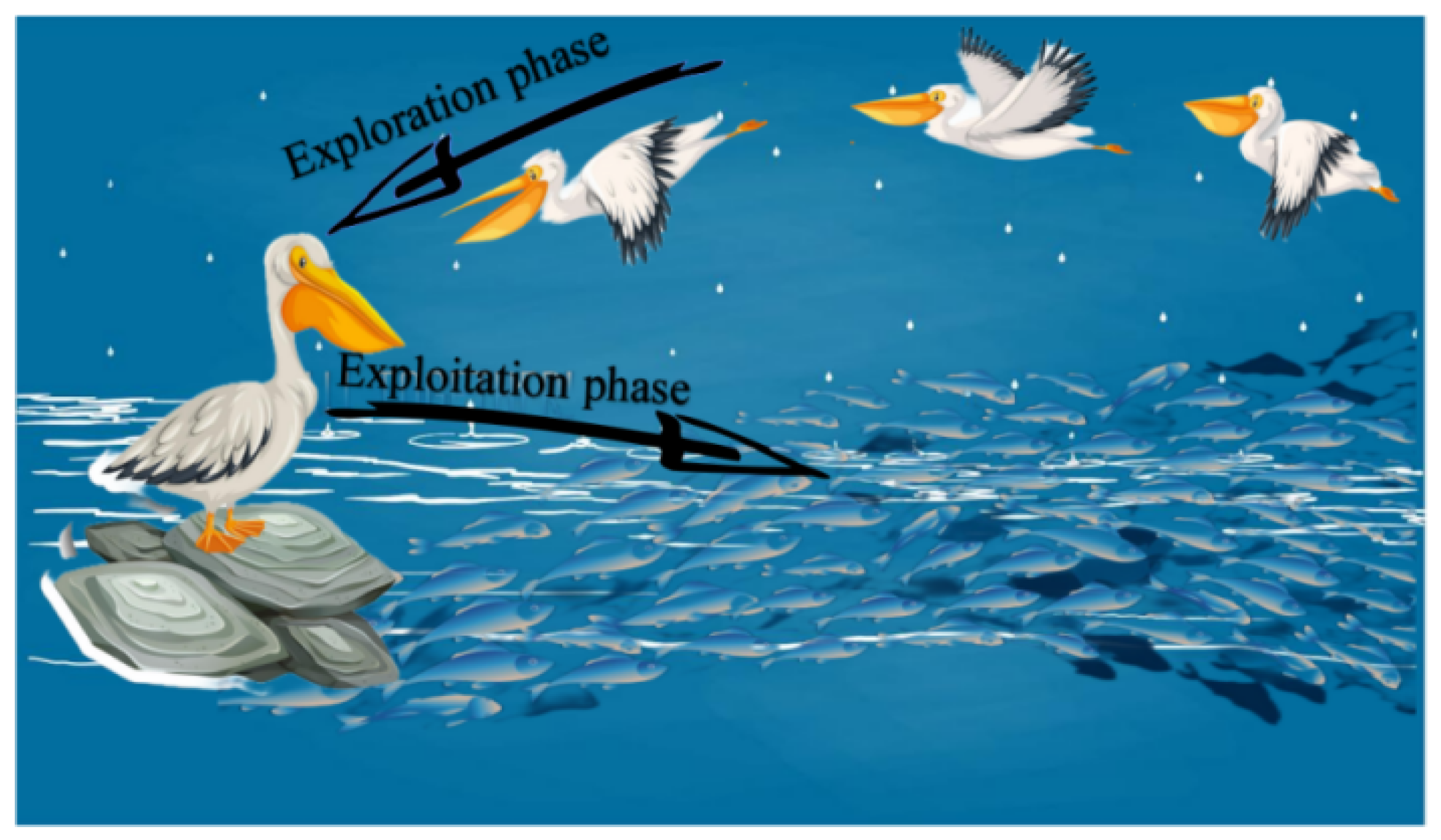
Figure 1. Search mechanism of POA.
Forests 15 01783 g001
Figure 2. The dot plot of w and r a n d . (a) r a n d dot plot. (b) w dot plot.
Forests 15 01783 g002
Figure 3. Schematic diagram of Hardy–Weinberg.
Forests 15 01783 g003
Figure 4. Trajectory of Levy flight and exponential Levy flight. (In (b), yellow represents Levy flight, blue represents [47], black represents [48], green represents [49], red represents Exponential Levy flight).
Forests 15 01783 g004
Figure 5. Canopy images of forests under different types of illumination.
Forests 15 01783 g005
Figure 6. Four typical curves of the grayscale transformation function. (a) Expand the darker areas. (b) Expand the brighter areas. (c) Stretch the middle and compress both ends. (d) Stretch both ends and compress the middle.
Forests 15 01783 g006
Figure 7. Variation of enhancement curves for different values.
Forests 15 01783 g007
Figure 8. Plot of enhancement results for low-illumination forest canopy images at different values of γ .
Forests 15 01783 g008
Figure 9. Results of sky enhancement for different parameters.
Forests 15 01783 g009
Figure 10. Flowchart of enhancement based on the MIPOA algorithm.
Forests 15 01783 g010
Figure 11. Convergence curves of each algorithm on the test function.
Forests 15 01783 g011
Figure 12. Plot of the enhancement results for each algorithm.
Forests 15 01783 g012
Table 1. Five POA improvement algorithms.
No.MethodAlgorithm Performance Improvement
 [28]Introducing the sine–cosine algorithm and linear weights w in the POA exploratory phaseImproving the population’s optimization accuracy
Perturbing the new individuals after the population iteration is completedIncreasing the convergence accuracy of the population
[29]Good point set initialization populationsImproving exploration capabilities
Inverse computation of pelican positions using reverse difference evolutionary algorithmFast approach to the optimal solution
Introducing an adaptive t-variation perturbation strategy near the optimal solutionImproving convergence accuracy and avoiding falling into local optimal solutions
[30]A new quality perturbation method is introduced. The principle is to converge to a better solution by detecting points near the distribution pointsEffectively improves the convergence accuracy of the POA algorithm when dealing with multi-peak functions
[31]Tent chaotic and refractive reverse learning strategies to initializing pelican populationsIncreasing the diversity of populations
Nonlinear inertia weighting factorsImproving the convergence speed of the algorithm
Leader strategy of the salp swarm algorithmCoordinate algorithm exploitation and exploration capabilities
[32]Initialization of pelican populations using Tent chaos mappingImproving the algorithm’s global search capability
The dynamic weighting factor θ helps the pelican particles to update their positions constantlyThe algorithm is motivated to perform a better localized search while speeding up convergence
Table 2. Information of benchmark functions.
StyleFunctionsDimRange f min
Unimodal F 1 ( x ) = i = 1 n 1 100 x i + 1 x i 2 2 + x i 1 2 30[−30,30]0
F 2 ( x ) = i = 1 n x i + 0.5 2 30[−100,100]0
Multimodal F 3 ( x ) = π n 10 sin π y 1 + i = 1 n 1 y i 1 2 1 + 10 sin 2 π y i + 1 + y n 1 2 + i = 1 n u x i , 10 , 100 , 4 y i = 1 + x i + 1 4 , u ( x , a , k , m ) = k x i a m x i > a 0 a < x i < a k x i a m x i < a 30[−50,50]0
F 4 ( x ) = 0.1 sin 2 3 π x 1 + i = 1 n x i 1 2 1 + sin 2 3 π x 1 + 1 + x n 1 2 1 + sin 2 2 π x n + i = 1 n u x i , 5 , 100 , 4 30[−50,50]0
Fixed-
dimension
F 5 ( x ) = i = 1 5 x a i x a i T + c i 1 4[0,10]−10.1532
F 6 ( x ) = i = 1 7 x a i x a i T + c i 1 4[0,10]−10.4028
Table 3. Comparison of optimization results for different values of parameter d.
d0.10.30.50.70.9 rand
F 1 2.7113 × 10 18 1.094 × 10 15 1.5555 × 10 19 2.0785 × 10 16 1.1022 × 10 9 1.2738 × 10 6
F 2 2.0009 × 10 31 4.2761 × 10 31 000 1.7804 × 10 20
F 3 3.7121 × 10 31 5.6552 × 10 31 3.7108 × 10 31 1.5452 × 10 31 1.1499 × 10 30 1.4978 × 10 15
F 4 4.6631 × 10 31 1.3703 × 10 32 5.4507 × 10 32 1.0934 × 10 30 5.8286 × 10 32 1.4723 × 10 22
F 5 −10.1532−10.1532−10.1532−10.1532−10.1532−10.1532
F 6 −10.4028−10.4028−10.4028−10.4028−10.4028−10.4028
Table 4. Mean fitness values of test functions.
FunctionIPOA1IPOA2IPOA3IPOA4IPOA5POAMIPOA
F 1 6.8457.71618.02527.76146.46866.3346 1.53 × 10 17
F 2 3.75 × 10 3 0.509310.936830.245650.105870.141880
F 3 1.14 × 10 3 6.64 × 10 2 0.24127 3.92 × 10 2 8.37 × 10 3 2.83 × 10 2 7.47 × 10 32
F 4 5.05 × 10 3 0.522240.498320.27030.230570.33185 5.19 × 10 30
F 5 −7.4037−10.151−3.824−8.4475−9.471−9.6433−10.1532
F 6 −8.152−10.4008−3.6839−9.8673−10.2244−8.9854−10.4028
Table 5. Means of Variance of Test Functions.
FunctionIPOA1IPOA2IPOA3IPOA4IPOA5POAMIPOA
F 1 0.388830.85020.242780.188440.571320.68305 7.11 × 10 17
F 2 2.54 × 10 3 0.26420.14960.197210.145710.154220
F 3 7.97 × 10 4 4.90 × 10 2 6.14 × 10 2 3.25 × 10 2 1.50 × 10 2 6.19 × 10 2 1.33 × 10 31
F 4 5.30 × 10 3 0.243740.103860.206680.17580.19504 2.84 × 10 29
F 5 2.4497 3.67 × 10 3 0.52962.43981.76171.5555 3.98 × 10 7
F 6 2.5498 3.30 × 10 3 0.777421.62050.970182.3906 4.62 × 10 5
Table 6. p-values of the Wilcoxon rank–sum test over 30 runs ( p > 0.05 has been in bolded).
  FunctionMIPOA vs.
IPOA1
MIPOA vs.
IPOA2
MIPOA vs.
IPOA3
MIPOA vs.
IPOA4
MIPOA vs.
IPOA5
MIPOA vs.
POA
F 1 1.27 × 10 11 2.52 × 10 11 1.79 × 10 11 1.96 × 10 11 2.63 × 10 11 2.40 × 10 11
F 2 1.21 × 10 12 2.37 × 10 12 1.21 × 10 12 1.72 × 10 12 3.16 × 10 12 1.72 × 10 12
F 3 6.48 × 10 12 3.16 × 10 12 1.21 × 10 12 5.22 × 10 12 3.16 × 10 12 1.72 × 10 12
F 4 1.72 × 10 12 1.72 × 10 12 2.37 × 10 12 4.11 × 10 12 3.16 × 10 12 3.16 × 10 12
F 5 2.79 × 10 11 2.85 × 10 11 2.94 × 10 11 2.91 × 10 11 4.97 E 10 4.41 × 10 7
F 6 2.98 × 10 11 2.98 × 10 11 3.01 × 10 11 2.86 × 10 11 1.23 × 10 7 7.61 × 10 5
Table 7. The FSIM value obtained by each intelligent algorithm.
ImagePSOChOAFAGHWOAPOAMIPOA
L10.41960.74090.64500.64570.64440.7409
L20.78910.75420.78630.78660.78610.7872
L30.47150.87290.47150.47150.47150.8729
L40.68130.75440.67630.68550.67620.7782
N10.45450.55740.45450.45450.45450.5574
N20.45410.69550.63680.63520.63980.6955
N30.42080.73660.65780.66410.65890.7366
N40.45780.68340.61920.74650.62860.6834
S10.66110.67280.66230.66240.66230.6728
S20.71710.70720.70230.70240.70590.7072
S30.72280.74720.72320.74530.73180.7472
S40.47020.527750.67310.503910.67220.6735
Table 8. The entropy value obtained by each intelligent algorithm.
ImagePSOChOAFAGHWOAPOAMIPOA
L10.60200.60950.60930.60950.60200.9963
L21.04961.04911.03291.03291.03291.0680
L30.72380.72380.72380.72380.72381.2062
L41.09061.09980.98761.10066.18945.4951
N10.75250.75250.75250.75250.75250.7525
N20.68890.68890.68890.68890.68890.7093
N30.65520.66570.67170.67170.67171.0131
N40.70210.70210.70210.94930.70210.7223
S10.89120.81170.81170.81170.81170.8999
S21.02370.88140.91140.93900.94630.9464
S30.95100.99330.95100.97770.96430.9977
S40.56890.62310.62060.62060.62060.6206
Table 9. The CII value obtained by each intelligent algorithm.
ImagePSOChOAFAGHWOAPOAMIPOA
L10.134130.365430.354050.356550.352530.75717
L20.86210.873180.836810.838710.835480.87162
L30.232880.232880.232880.232880.232880.7.552
L40.520040.530580.501190.535360.368670.56017
N10.273330.273330.273330.273330.273330.32986
N20.241850.241490.358720.356210.361040.46825
N30.189880.424050.435980.450270.438410.72213
N40.251920.251480.371940.355150.382550.49493
S10.559910.547690.539670.541020.540450.58361
S20.810390.668210.698070.702010.724160.73274
S30.700630.611530.702290.822810.744410.82672
S40.138440.527750.486580.503910.482610.48858
Table 10. The pixel mean values obtained by each enhancement algorithm.
ImageSSRMSRCRHEAHEESIHEAGCWDPOAMIPOA
L10.17380.13045131.802667.8067146.48662.3378136.4606109.3775
L20.17190.13563133.548968.4875146.161767.1037110.8766111.2707
L30.155340.12036134.717964.849148.569562.4672168.6012120.3972
L40.185980.22468131.467672.198146.795865.8371116.2406101.3712
N10.158720.1227135.412566.5866150.659761.5617188.433102.1638
N20.176230.12525133.67272.8189150.854262.2017152.677699.47
N30.188770.13811132.701775.5299150.619265.7029136.6966122.2561
N40.176760.11069133.892371.693150.845662.4132150.379897.7514
S10.209910.13783130.43276.9887144.823359.4392109.4696116.9768
S20.223190.15324129.668978.1447143.547564.667689.511695.4927
S30.258790.18499131.103687.7792149.562567.4396105.4981105.9425
S40.188710.129131.970969.6043144.961259.185997.461113.904
Table 11. The average gradient value obtained by each enhancement algorithm.
ImageSSRMSRCRHEAHEESIHEAGCWDPOAMIPOA
L10.214760.2056869.112489.466561.472977.697979.995999.7079
L20.190320.1806356.236375.9450.70767.68973.280973.0566
L30.173490.175657.484776.279651.337868.457246.991776.4251
L40.227960.2246864.559891.16656.978179.20596.3159103.6209
N10.195550.196659.372586.527652.3575.805120.610890.2516
N20.247220.2283377.0218103.764166.94589.360572.1111122.0603
N30.265270.2452880.1178112.757469.294895.120799.7179115.1481
N40.249520.1993379.3524106.994869.288491.05277.5816126.5218
S10.235570.2008864.187585.727357.229267.980990.423993.6418
S20.228380.1944759.666783.601753.929663.494287.794787.8751
S30.326790.3051977.4858109.907367.006294.2225123.0046123.2372
S40.223590.1973958.66883.709452.961169.383986.732596.788
Disclaimer/Publisher’s Note: The statements, opinions and data contained in all publications are solely those of the individual author(s) and contributor(s) and not of MDPI and/or the editor(s). MDPI and/or the editor(s) disclaim responsibility for any injury to people or property resulting from any ideas, methods, instructions or products referred to in the content.