Simple Summary
Wood-boring pests pose a significant threat to the health of trees in forest and urban ecosystems. Their larvae live deep within the xylem of tree trunks, where visible signs of their activity on the trunk surface are minimal. Traditional monitoring methods are time-consuming and labor-intensive, making it difficult to detect infestations early, thereby complicating pest control efforts. Taking the emerald ash borer (EAB), Agrilus planipennis Fairmaire, 1888 (Coleoptera: Buprestidae), and the small carpenter moth (SCM), Streltzoviella insularis Staudinger, 1892 (Lepidoptera: Cossidae), commonly found on ash trees (Fraxinus chinensis Roxb) in northern China, as examples, acoustic sensors can be used to collect the feeding vibration signals of their larvae, providing a new approach to pest identification. This paper proposes a deep learning recognition model, BorerNet, which uses these boring vibration signals as input and incorporates an attention mechanism. Experimental results show that this model achieves high recognition accuracy. The method can provide technical support for the identification and control of wood-boring pests.
Abstract
Wood-boring pests are difficult to monitor due to their concealed lifestyle. To effectively control these wood-boring pests, it is first necessary to efficiently and accurately detect their presence and identify their species, which requires addressing the limitations of traditional monitoring methods. This paper proposes a deep learning-based model called BorerNet, which incorporates an attention mechanism to accurately identify wood-boring pests using the limited vibration signals generated by feeding larvae. Acoustic sensors can be used to collect boring vibration signals from the larvae of the emerald ash borer (EAB), Agrilus planipennis Fairmaire, 1888 (Coleoptera: Buprestidae), and the small carpenter moth (SCM), Streltzoviella insularis Staudinger, 1892 (Lepidoptera: Cossidae). After preprocessing steps such as clipping and segmentation, Mel-frequency cepstral coefficients (MFCCs) are extracted as inputs for the BorerNet model, with noisy signals from real environments used as the test set. BorerNet learns from the input features and outputs identification results. The research findings demonstrate that BorerNet achieves an identification accuracy of 96.67% and exhibits strong robustness and generalization capabilities. Compared to traditional methods, this approach offers significant advantages in terms of automation, recognition efficiency, and cost-effectiveness. It enables the early detection and treatment of pest infestations and allows for the development of targeted control strategies for different pests. This introduces innovative technology into the field of tree health monitoring, enhancing the ability to detect wood-boring pests early and making a substantial contribution to forestry-related research and practical applications.
1. Introduction
With the global trend toward sustainable development, forestry construction has gradually become a topic of common concern among countries. Forest ecosystems play a crucial role in the global environment, particularly in protecting biodiversity, mitigating global climate change, maintaining soil and water resources, and enhancing socioeconomic benefits [1,2]. Additionally, in modern cities, urban greening is also indispensable. It plays a vital role in improving air quality, regulating climate, reducing noise, beautifying the environment, and increasing economic value, thereby comprehensively enhancing urban sustainability and livability [3]. The white ash tree is widely distributed in North America and in Asian regions such as China, Japan, and Korea. It is known for its good cold and drought resistance and is a common urban greening species [4].
Various pests pose a serious threat to forests and urban greening. They can spread rapidly and damage plant health, leading to widespread tree mortality and reducing the ecological functions of forests and urban green spaces [2]. Among the various types of insect infestations that trees endure, wood-boring insects are particularly harmful and insidious, making them one of the most challenging pests to control in China’s forestry pest management [5]. The larvae of these insects bore into the interior of trees, damaging the conductive tissues, which leads to the weakening or even death of the trees [6]. The feeding behavior of wood-boring insects leaves wounds inside trees, which can easily become entry points for pathogens such as fungi and bacteria [7,8]. The large-scale reproduction and spread of wood-boring insects can have widespread effects on forest ecosystems. The mass die-off of trees not only alters the species composition and structure of forests but also affects the habitats and food sources of other flora and fauna within the forest. After trees die, the fallen deadwood on the forest floor increases the risk of forest fires [9]. The emerald ash borer (EAB), Agrilus planipennis Fairmaire, 1888 (Coleoptera: Buprestidae), and the small carpenter moth (SCM), Streltzoviella insularis Staudinger, 1892 (Lepidoptera: Cossidae), are two important wood-boring pests, causing extensive damage to economically valuable tree species and forest resources. Their impact not only results in economic losses but also disrupts the balance of ecosystems [10,11].
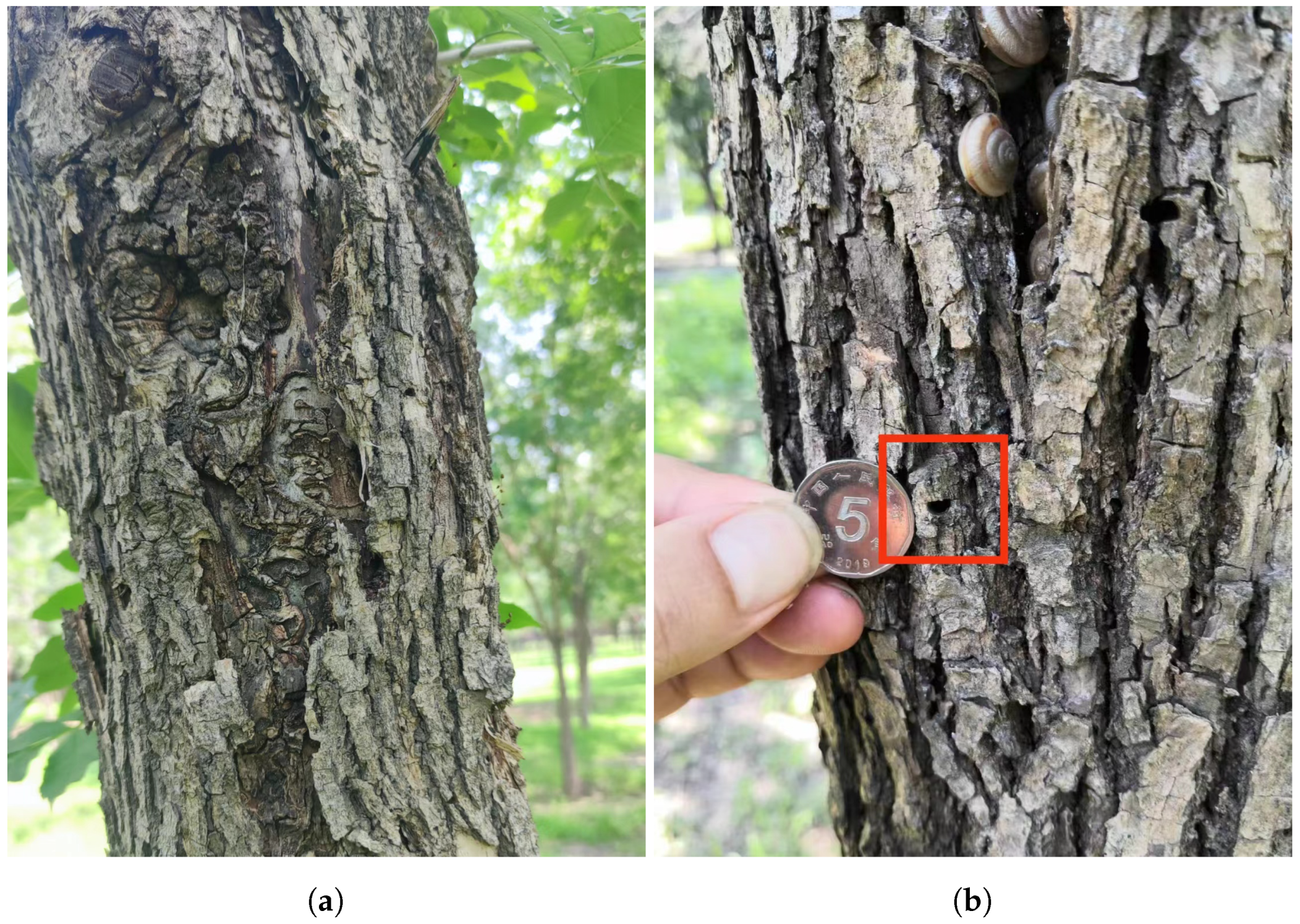
Agrilus planipennis, originally native to East Asia, invaded North America in the late 20th century, spreading rapidly and causing severe ecological and economic impacts. EAB larvae bore through the phloem, cambium, and outer xylem layers of trees, creating irregular galleries that disrupt the tree’s ability to transport water and nutrients from the roots to the upper parts of the tree [11]. The U.S. Department of Agriculture estimates that, since its discovery, the EAB has killed tens of millions of ash trees, resulting in economic losses amounting to billions of dollars [10,12,13,14]. In the Chinese Beijing area, EAB larvae hatch in June, with their activity period lasting from July to mid-August. The adult exit holes are “D”-shaped. Evidence of their activity is shown in Figure 1.

Figure 1.
Evidence of Agrilus planipennis activity. (a) Galleries created by Agrilus planipennis due to prolonged feeding. (b) D-shaped exit hole left after Agrilus planipennis emerges.
The main methods for controlling the EAB include the application of chemical agents, such as Avermectins, which can be administered through trunk injection to kill larvae feeding on the tree trunk [15]. In addition, insecticides can be sprayed on the tree canopy and trunk during the adult flight period to kill adults and prevent them from laying eggs [16]. In the EAB’s native habitat, researchers have identified parasitic wasps, such as Oobius agrili Zhang and Huang, 2010 (Hymenoptera: Encyrtidae), that can be used as a biological control method. These wasps parasitize EAB eggs and larvae, thereby reducing their population [17]. For severely infected ash trees, especially in the early stages of an outbreak, the timely felling and removal of infected trees can help prevent the spread of the pest. Additionally, planting rotations and selective tree planting can be employed to reduce suitable habitats for this pest [10,11].
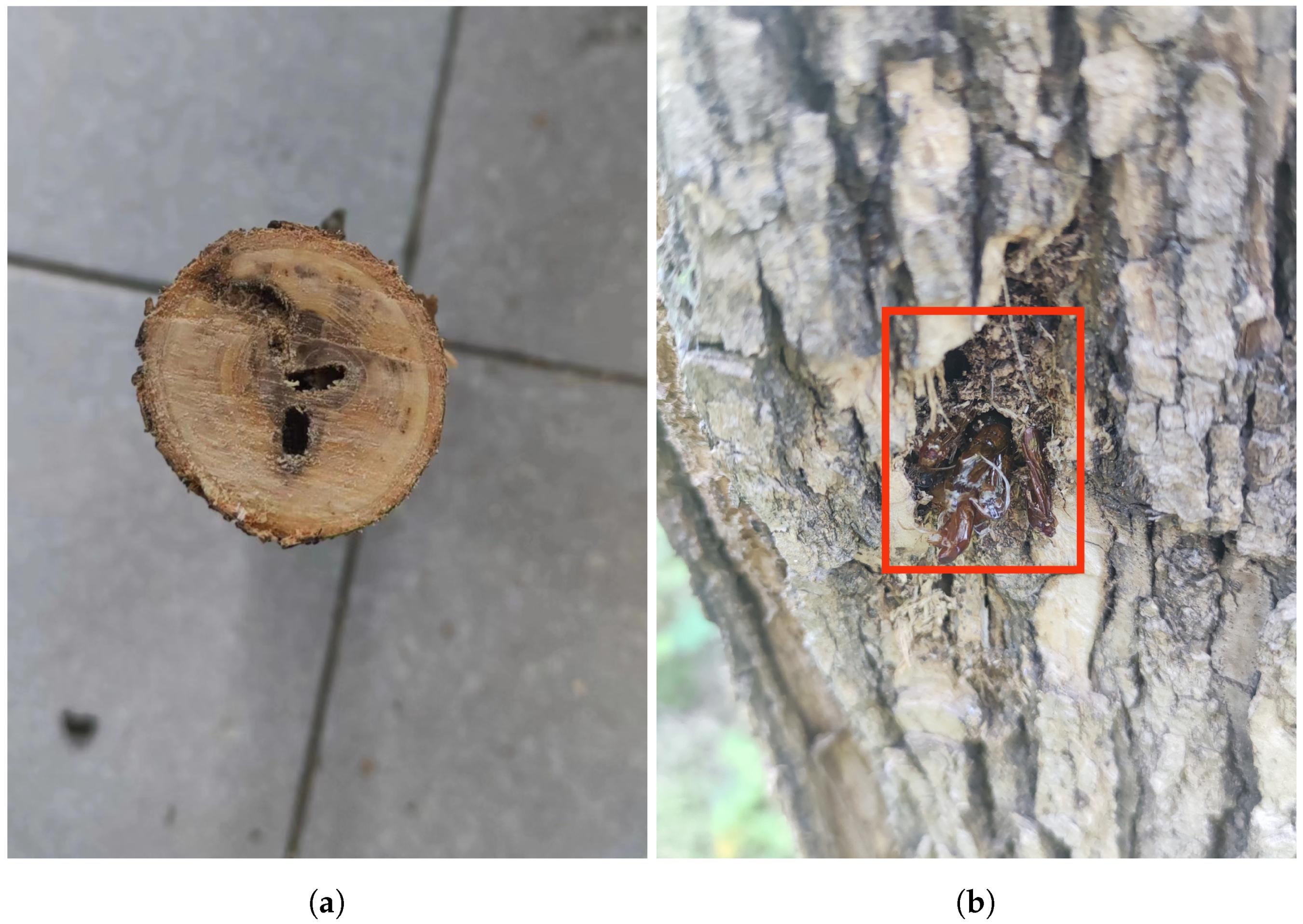
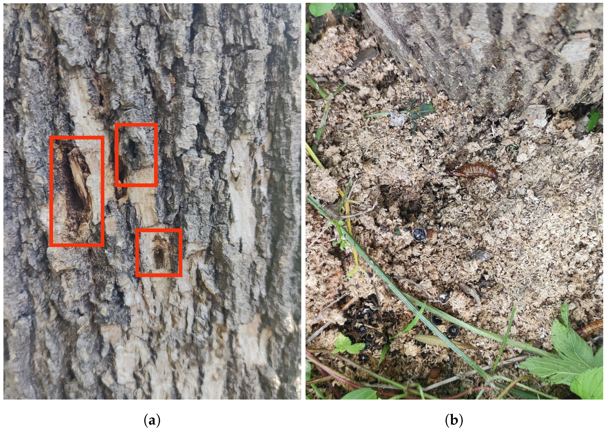
Streltzoviella insularis is widely distributed across Europe and Asia, causing severe damage to various fruit trees and forest trees. SCM larvae bore into tree trunks and branches, forming galleries that can house dozens to hundreds of larvae. This results in extensive tunneling, severely compromising the structure and health of the tree, leading to stunted growth, reduced yield, and even tree death. The galleries of the SCM are interconnected, with external boreholes often linked by silk-bound, spherical frass. In addition to the direct damage caused, SCM infestations also weaken the tree’s resistance to other pests and diseases, making it more susceptible to secondary infestations [18]. The impact on fruit trees, such as apple trees (Malus domestica) [19], is particularly severe, affecting both the yield and quality of the fruit [20,21]. The SCM has a two-year life cycle, with larvae hatching in June, pupating in July, and emerging as adults from late July to mid-August. Evidence of their activity is shown in Figure 2.

Figure 2.
Evidence of Streltzoviella insularis activity. (a) Boreholes observed after cutting open the tree trunk. (b) The pupal cases and exit holes left on the tree trunk surface after Streltzoviella insularis emerges.
The main methods for controlling the SCM include plant quarantine, physical control, biological control, and chemical control. Plant quarantine requires immediate pest management or the destruction of any seedlings, logs, or wood infested by the little leaf borer moth during routine inspections to prevent further outbreaks. Some physical control measures involve the timely pruning and removal of severely affected branches and underground debris during winter, which should be concentrated and destroyed to reduce pathogen sources. During the adult emergence period, a certain number of solar insecticidal lamps can be installed in forest areas and orchards to attract and electrically kill adult insects. Biological control involves introducing natural enemies of the SCM, such as woodpeckers and the entomopathogenic fungus Beauveria bassiana. Chemical control refers to spraying insecticides on tree trunks and leaves during the adult emergence period or injecting insecticides into the burrows during the larval stage [22].
Pest species identification is crucial in Integrated Pest Management (IPM) because it forms the foundation for developing effective control strategies. Accurate identification helps in selecting targeted control measures, such as biological, physical, or chemical methods, thereby avoiding indiscriminate pesticide use, which reduces environmental pollution and harm to beneficial organisms. Moreover, correct pest identification prevents resource waste, delays the development of pest resistance, and ensures that control measures are applied at the most critical stages of the pest’s life cycle. Therefore, precise pest identification is a core step in the successful implementation of IPM [23].
Our preliminary research has revealed that many of these trees in urban areas are infected by the EAB and SCM. If not treated, the infected trees face the threat of death within three years, leading to significant economic losses. The larvae of the EAB and SCM primarily damage the tree trunks and branches, with the larval stage causing the most severe destruction. The vibrations produced by the feeding activities of the larvae provide an ideal basis for developing a monitoring model. Traditional monitoring methods for wood-boring insects primarily rely on manual inspections and chemical detection. Manual inspections require experienced professionals to conduct on-site examinations, which are time-consuming and labor-intensive, making large-scale, efficient monitoring difficult to achieve. The use of chemical pesticides can lead to environmental pollution, harm non-target organisms, and contribute to the development of pest resistance issues [14,24]. As noted by Kovacs et al. [25], the larvae of the EAB typically show few or no signs of infestation during the early stages, making it challenging to detect the presence of pests before significant tree mortality occurs. There is an urgent need to develop rapid and accurate monitoring and identification techniques for wood-boring insects. Improving the accuracy of pest identification offers significant advantages for pest control. It not only allows for more effective pest management and the protection of agricultural and forestry resources but also achieves both environmental and economic benefits. This paper addresses the practical need for monitoring wood-boring insects by combining vibration signal analysis and deep learning technology, developing an effective early detection solution that provides a new approach to tree health monitoring and ecosystem management.
2. Related Work
With the development of speech recognition technology, acoustic monitoring has emerged as a new method for pest detection. This approach primarily utilizes the activity of pests within trees for monitoring, offering advantages such as high efficiency, simplicity, low cost, and early warning capabilities, with promising potential for widespread application. In recent years, research on insect sound recognition has broadened, providing a solid foundation for identifying boring insects based on their boring vibration signals [26]. However, the current exploration of various sound signal features and algorithm models still faces significant limitations. There is a lack of systematic recognition processes, and recognition accuracy has room for improvement. Additionally, there is limited research on the performance of recognition from a time efficiency perspective and scant consideration of noisy boring vibration signals, which hampers practical application. Farr et al. [27] found that when the primary goal is to detect wood-boring insects, piezoelectric sensors are preferable to electret microphones due to their higher sensitivity. Therefore, this study employs piezoelectric sensors to capture boring vibration signals.
Whether dealing with boring vibration signals studied in this paper or various sounds encountered in daily life, both fundamentally involve the generation of mechanical waves due to object vibrations, which propagate through the surrounding air and are converted into audible sound by the human ear. Therefore, detection technologies suited for other types of sound are also applicable to boring vibration signals. The application of deep learning in acoustic recognition and classification dates back to early research on bat echolocation in the early 21st century. Since then, many traditional feature-extraction-based recognition methods have emerged [28]. For instance, Yazgaç B G et al. [29] used animal sound signals for the detection and control of grain pests. Njoroge et al. [30] employed microphones to record the sound signals produced by Prostephanus truncatus Horn (Coleoptera: Bostrichidae) and Sitophilus zeamais Motschulsky (Coleoptera: Curculionidae) during feeding and movement in corn. By analyzing metrics such as average pulse rate and average pulse count, they identified significant differences in pulse signals between adults and larvae at various developmental stages, facilitating pest detection in crops. Jalinas et al. [31] used Beauveria bassiana (Bals.-Criv.) Vuill. (Hypocreales: Clavicipitaceae) as a pathogen to infect the larvae of Rhynchophorus ferrugineus (Coleoptera: Dryophthoridae). They recorded the sound signals produced by the host during feeding and movement. They observed that the infected larvae showed significantly reduced feeding and movement times, demonstrating that Beauveria bassiana slows down larval movement and increases mortality.
In recent years, with technological development, sound detection technology has increasingly been applied to the study of wood-boring insects. A typical instrument for capturing boring vibration signals is the portable sound detector AED-2000/2010L from the American AEC company, which is equipped with the SP-1L contact probe. Experts, both domestic and international, have used the AED portable sound detector for research on wood-boring pests in agriculture and forestry. For instance, Herriick et al. [32] used the AED-2000 to capture the sounds of Rhynchophorus ferrugineus (Coleoptera: Curculionidae) and other palm-tree-damaging beetles. They assessed the data using least squares methods at the spectral level, finding that all larval stages could be detected at distances of at least 5–10 cm in both closed and open environments. Detection distances in closed environments were 2–4 times greater than those in open environments. Mankin et al. [33] studied the boring vibrations of Rhynchophorus ferrugineus (Coleoptera: Dryophthoridae) and another pest, Oryctes elegans Prell (Coleoptera: Scarabaeidae), in orchard environments where these pests frequently co-occur. They achieved automatic recognition of the two types of larvae. In a subsequent study, Mankin et al. [34] used a pest sound detection system to test avocado trees suspected of being infested by Mallodon dasystomus Say (Coleoptera: Cerambycidae). They correctly identified all four infested trees out of eleven tested, with only one false positive for a healthy tree. Eliopoulos et al. [35] conducted a study using a piezoelectric sensor connected to a portable acoustic emission amplifier linked to a computer to record insect sounds. They then used a linear model to describe the relationship between the number of pests and the recorded sound data. Additionally, Mankin et al. [36] employed acoustic devices to detect pests in stored products.
In recent years, deep learning technology has made significant advancements and has proven to be highly effective in addressing complex recognition and detection tasks. Deep learning models, through automatic feature extraction and pattern recognition, can extract useful information from complex vibration signals, significantly enhancing the accuracy and efficiency of signal processing [37]. In the field of pest monitoring, deep learning models can classify and identify different types of pests based on collected boring vibration signals, providing accurate pest monitoring data. For instance, Zhu et al. [38] utilized existing speech recognition parameterization techniques to identify pests. In their study, preprocessed audio data were used to extract Mel-frequency cepstral coefficients (MFCCs), which were then classified using a trained Gaussian Mixture Model (GMM). Sun et al. [39] proposed a lightweight convolutional neural network consisting of four convolutional layers, employing keyword spotting techniques to identify vibrations produced by Semanotus bifasciatus and Eucryptorrhynchus brandti larvae. Zhang et al. [40] employed a Visual Geometry Group 16 (VGG16)-based classification network for pest sound detection from boring vibration signals and confirmed the effectiveness of deep learning methods in denoising boring pest vibration signals. W. Jiang et al. [41] designed a convolutional neural network (CNN) network for the classification of boring pests. Dong et al. [42] proposed a PestLite model based on You Only Look Once v5 (YOLOv5), using Multi-level Spatial Pyramid Pooling technology to significantly improve detection accuracy while reducing model parameters. Similarly, Tang et al. [43] introduced an improved YOLO model that achieved real-time, efficient pest detection.
This study leverages computer deep learning technology by incorporating attention mechanisms to achieve the precise identification of wood-boring pest species using limited boring vibration signals. The main contributions of this work are as follows:
- (a)
- The Development of Self-Designed Equipment and Data Collection: Custom equipment was developed to collect boring vibration signals from the larvae of two target pests. Preprocessing of the raw signals was performed to construct an experimental dataset.
- (b)
- The Introduction of a Deep Learning-Based Recognition Model: A deep learning-based recognition model is proposed, which extracts MFCCs as input and incorporates the NAM attention mechanism, enabling accurate identification of wood-boring pests in noisy real-world environments.
- (c)
- Pest Control: A new approach to pest control is provided, allowing for precise control of different pests and aiding in the prediction of potential future pest problems, thereby improving control efficiency and reducing costs.
3. Data Collecting and Processing
3.1. Data Collecting
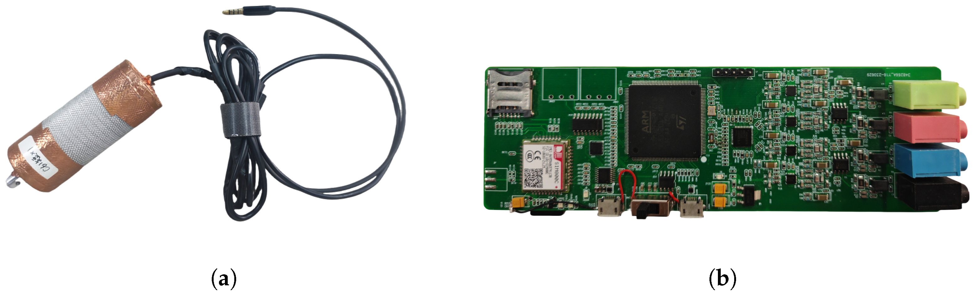
The subjects of this study are the larvae of the EAB and the SCM, with the experiment focusing on collecting the vibration signals generated as they feed within tree trunks. Since existing equipment could not meet the data collection requirements, a self-developed piezoelectric sensor developed jointly by Beijing Forestry University and Beihang University was used to capture clear and complete signals, as shown in Figure 3a. Before signal collection begins, the sensor probe is embedded into the tree trunk using an electric drill, after which it is connected to the collection device to monitor the vibration signals produced by the pests’ activity within the trunk. These signals are recorded in audio format (.wav). This method of embedding the probe into the trunk not only simplifies the signal collection process but also significantly enhances the purity of the captured signals. Additionally, the design is ingenious in that it only requires minimal embedding on the tree surface, avoiding extensive damage to the trunk and thereby preserving the tree’s integrity to the greatest extent possible.

Figure 3.
Data collection equipment. (a) Self-developed piezoelectric sensor. (b) Multi-channel signal acquisition device.
This project also involved the independent design and development of a multi-channel signal acquisition device, as shown in Figure 3b. The device significantly enhances data collection efficiency and creates favorable conditions for achieving multi-channel signal enhancement. By leveraging the multi-channel capability, signals can be synthesized and enhanced, resulting in clearer and more reliable final outputs. Additionally, the device can be powered by a portable power source, making it more adaptable to forest environments compared to a PC. The signal acquisition device features four channels with a maximum amplification gain of 100×, a sampling rate of 44.1 kHz, and a passband range of 20 Hz to 20 kHz. It is capable of simultaneously sampling and saving data from all four channels. The main CPU of the device is the STM32F429, equipped with SDRAM to increase the device buffer capacity. Data are saved using a high-speed SD card, with the ADAU1979 chosen as the analog-to-digital converter (ADC) to improve the sampling speed and accuracy of each channel. On the software side, Direct Memory Access (DMA) technology is employed to transfer data directly from the hardware device to memory, reducing the load on the CPU. Increasing the DMA buffer can reduce pauses or delays caused by asynchronous data transfer, thereby maximizing data integrity. A modular design approach allows each module to operate independently, facilitating upgrades and maintenance.
To ensure that the extracted signal features are representative, signal collection in this study was conducted over a three-year period, generating various types of data, which were organized into four categories, as shown in Table 1.

Table 1.
The types of signals collected in three years.
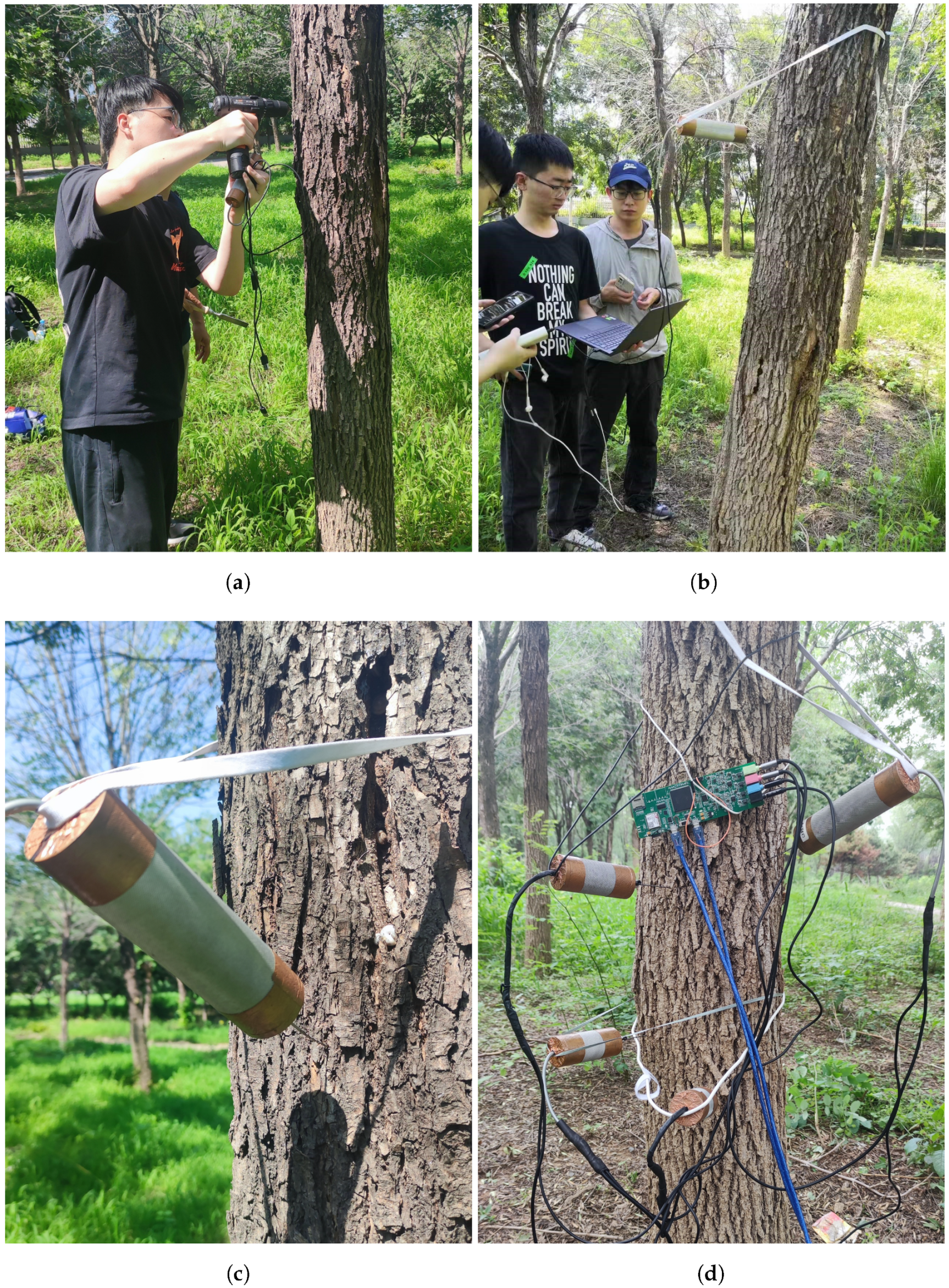
In Beijing, July and August are the active periods for the target pest larvae, with hotter weather facilitating noticeable insect activity, which is conducive to data collection for model training. The collection of vibration signals from the feeding larvae of the EAB began on 18 July 2022 and continued for five days. During this period, the average daytime temperature in the target forest area affected by EAB larvae in Shunyi District, Beijing , was approximately 33 °C. The forest environment where the data were collected is shown in Figure 4. The trees in the forest area are between 10 and 15 years old, with a diameter at breast height (DBH) of approximately 20 cm. The equipment required for signal collection included a piezoelectric sensor, a multi-channel signal acquisition device, a portable power source, data cables, a power drill, drill bits, and so on. The process began by identifying trees with noticeably poorer growth and inspecting their trunks. If “D”-shaped exit holes were found, the tree was preliminarily confirmed as being infested by the EAB and was marked. Before formal recording, the probe of the piezoelectric sensor was embedded about 2 cm into the trunk. The larvae’s activity was monitored using headphones, as shown in Figure 5a,b. Once vibration signals were confirmed, recording began, with each session lasting approximately 2 h per day. Figure 5c,d show the process of collecting signals in the forest using the piezoelectric sensor and multi-channel acquisition device.
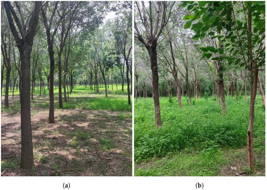
Figure 4.
The forest environment affected by an EAB infestation. (a) Weijiadian Village. (b) Xianggezhuang Village.

Figure 5.
(a) Embedding the probe into the tree trunk using a power drill. (b) Monitoring larval activity. (c) Capturing signals using a piezoelectric sensor. (d) Collecting signals using a multi-channel acquisition device.
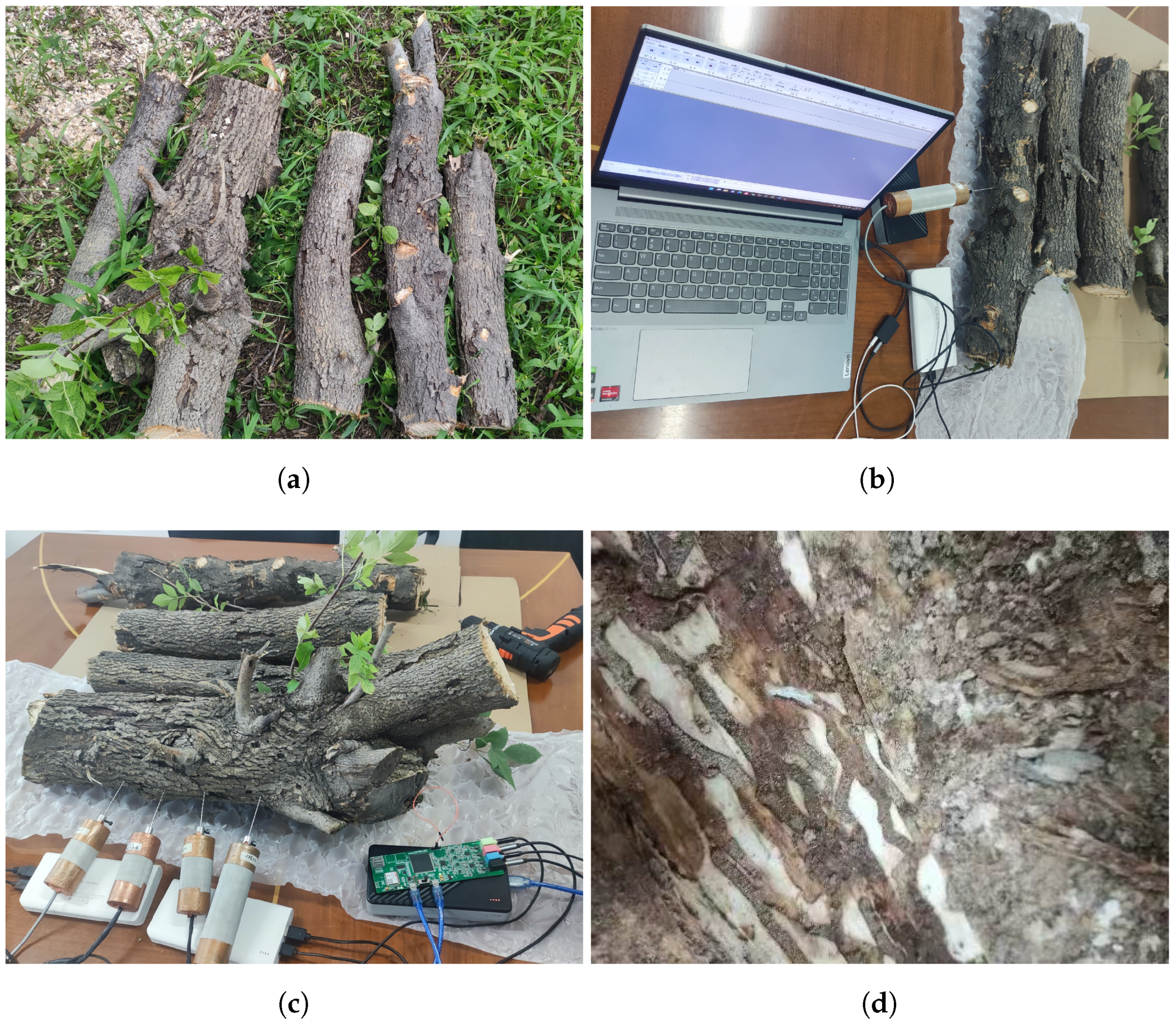
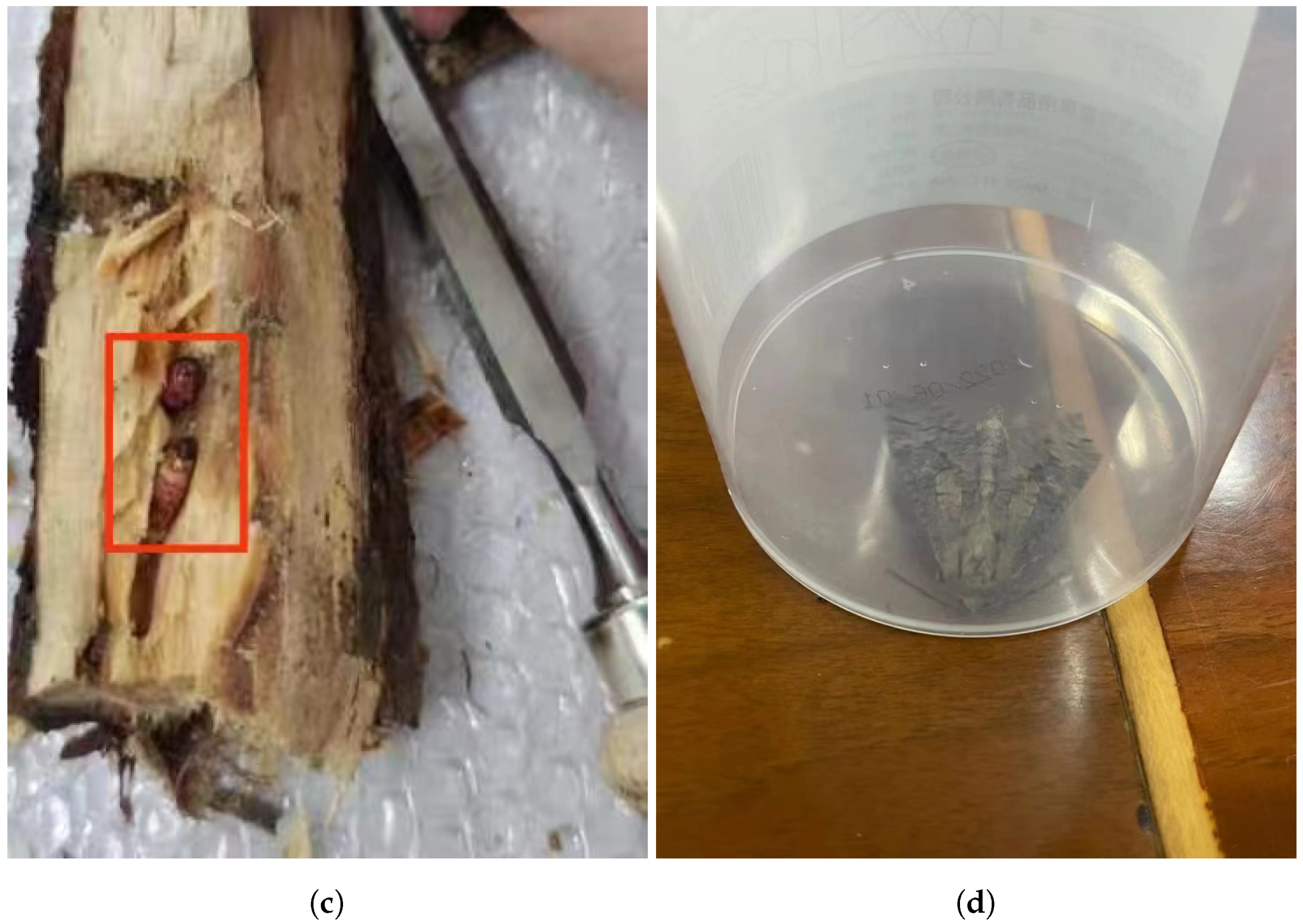
To meet the experimental requirements, it was necessary to collect signals in an environment free of ambient noise. With the assistance of forestry staff, a few carefully selected infested trees were felled and transported to a soundproof indoor environment, where the temperature was approximately 28 °C. Each tree segment measured between 60 and 100 cm in length and between 12 and 20 cm in diameter, as shown in Figure 6a. Observations revealed no SCM larval tunnels on the cross-sections of the felled tree trunks. Before recording, larval activity was monitored using headphones, just as in the forest setting. Once recording began, all personnel exited the soundproof room to minimize noise. If the larvae remained active within the tree segments, approximately 2 h of vibration data were recorded each day, capturing multiple audio segments from different parts of a single tree trunk. As a control, the dataset also included recordings from two tree segments without EAB larvae. For these segments, most recordings contained only the background noise of the equipment, as no larval activity was present. Recording began on 23 July 2022 and continued for five days. Figure 6b,c illustrate the process of collecting signals in the soundproof room using the piezoelectric sensor and multi-channel acquisition device. After recording was completed, under the supervision of forestry professionals, the bark was stripped from all tree segments to expose and count the EAB larvae, as shown in Figure 6d. Between 5 and 10 larvae were found in two segments, while the other four segments contained 10 to 20 larvae each, with the larvae measuring approximately 3 cm in length.
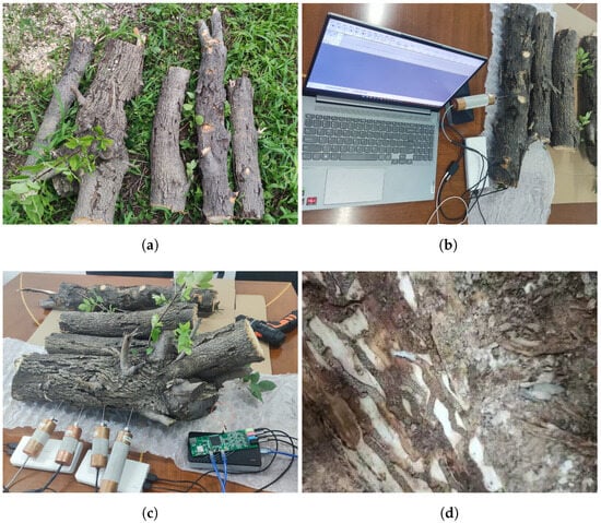
Figure 6.
(a) Cross-sections of tree trunks infested with Agrilus planipennis. (b) Monitoring boring vibration signals within the tree trunk. (c) Collecting Agrilus planipennis boring vibration signals in a soundproof room using a multi-channel acquisition device. (d) Counting the number of larvae within the tree trunks.
Streltzoviella insularis larval vibration signal collection began on 24 July 2023 and lasted for 5 days in a forest area in Shunyi District, Beijing. Preliminary research indicated that the forest area had a high prevalence of the SCM, with the average temperature during the signal collection period being approximately 34 °C. First, we conducted an initial screening of trees that were showing poor growth conditions. If exit holes are found on the trunk and there is noticeable wood debris at the base of the tree, it is highly likely that the tree is infected with the SCM. Then, we marked it accordingly, as shown in Figure 7a,b. The larvae measured approximately 4 cm in length, as shown in Figure 7c,d.
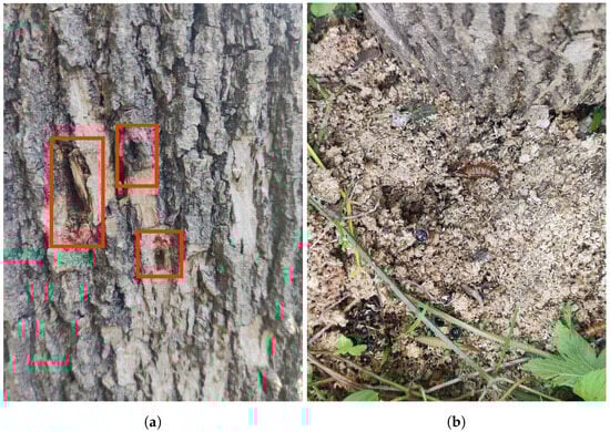

Figure 7.
(a) Streltzoviella insularis creates exit holes on the tree trunk. (b) The wood debris produced by Streltzoviella insularis boring. (c) Streltzoviella insularis larvae found inside a split tree trunk. (d) Captured adult Streltzoviella insularis beetles.
The third data collection began on 19 July 2024 in a forest area located in Shunyi District, Beijing. During the signal collection period, the average temperature in the forest area was approximately 34 °C. Vibration signals of SCM larvae feeding were collected, with the process divided into two stages: collection in the forest area and in a soundproof chamber. The collected signals were primarily used to expand the dataset, enhancing its representativeness and randomness.
3.2. Data Preprocessing
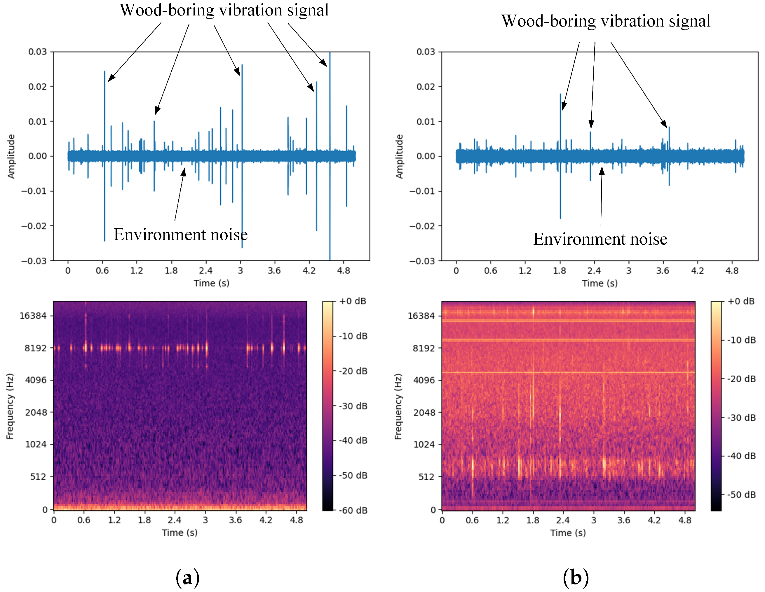
A single white ash tree may be simultaneously infected by both the EAB and SCM [44]. To better distinguish between the drilling vibration signals of these two pests and ensure the collected signals are as pure as possible, this study targeted white ash trees infected by only one of the pests during the data collection process. A computer program was developed to simulate the simultaneous presence of both pests by combining the drilling vibration signals of the two pests in a 1:1 ratio to generate a new signal, referred to as the EAB + SCM drilling vibration signal. The dataset includes four categories: vibration signals from EAB larvae and SCM larvae in both indoor and outdoor environments, computer-synthesized mixed signals, and isolated environmental noise data. The environmental noise primarily consists of sounds from wind, cicadas, and bird calls typical of summer forest environments. The waveforms and spectrograms are shown in Figure 8. By analyzing the collected vibration signals, it is easy to observe that these signals are composed of multiple discrete pulses, characterized by short bursts of high energy and brief duration, with relatively concentrated frequencies. In contrast, environmental noise lacks prominent peaks and has dispersed frequencies. Additionally, there are gaps in the signals, which may be due to the uneven activity of the pests. Besides these characteristics, careful listening reveals a small amount of background noise from the equipment in the signals.
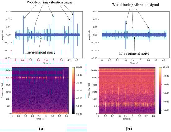
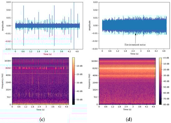
Figure 8.
Waveforms and spectrograms of the four types of signals. (a) Agrilus planipennis boring vibration signal. (b) Streltzoviella insularis boring vibration signal. (c) Agrilus planipennis + Streltzoviella insularis boring vibration signal. (d) Environmental noise.
Therefore, before using the dataset for training, a series of preprocessing operations was necessary for these signals, including clipping out the signal gaps in the audio files and denoising the equipment noise present in the recordings. Specifically, by manually observing the signal waveform, segments of non-boring vibration signals were identified and removed. These segments primarily included artificial noises generated at the beginning and end of each audio file during the process of turning the recording equipment on and off, as well as segments where insect activity was not evident. Only segments with clear EAB and SCM larval activity were retained. To minimize equipment noise, the Audacity software V3.33 was used to remove background noise. Since the boring vibration signals can vary daily due to changes in larval growth, emergence, and mortality, efforts were made to use a portion of the data collected each day to maximize the utilization of these data. After the aforementioned processing, a clean and dense boring vibration signal dataset was ultimately obtained.
Considering the precision of feature extraction and computational resource limitations, the aforementioned data were uniformly segmented, with each audio segment set to a length of 5 s. Additionally, the large volume of audio data significantly slowed down the computation speed and could potentially cause interruptions during training. To address this issue, multiple folders were created to store these audio segments for training, with each folder containing 500 audio segments. The dataset was then split into training and testing sets in a 7:3 ratio, followed by the generation of label files. The training set was sourced from noise-free larval boring vibration signals collected in a soundproof room, ensuring that the model could extract a more comprehensive range of signal features. To enhance the robustness of the detection model, the test set was sourced from real-world, noise-containing larval boring vibration signals. More precisely, in real-world scenarios, models may encounter various noisy environments, and the signals collected in the training set may not fully represent all possible situations. Using noise-free recording as the training dataset enables the model to learn the core features of the data under ideal conditions, without the interference of environmental noise. By doing so, the model can capture the essence of the data, allowing it to better understand the truly useful information within the signal. This helps the model maintain strong performance when dealing with unknown, noisy environments. If the training set includes environmental noise, the model might learn irrelevant or random features present in the noise, leading to overfitting. This means the model could perform well on noisy data but poorly on new data without those specific noisy features. In other words, a clean training set allows the model to focus on key, more general features of the signal, rather than adapting to particular noise patterns. This makes the model more stable when tested against noisy datasets or real-world data. It also allows for a better evaluation of the model’s robustness and generalization in complex, real-life environments. This approach strikes a balance between complexity in training and testing, aiding in the development of more stable and practical models. The dataset labeling is shown in Table 2, with the training set labeled as set = 1, and the test set as set = 0. The labels for the signals are as follows: environmental noise T = 0, EAB larval vibration signal T = 1, SCM larval vibration signal T = 2, and the simulated mixed vibration signal of EAB and SCM larvae T = 3. All of these operations were implemented through custom computer programs.
Table 2.
Dataset label allocation.
4. Methods
4.1. MFCC Feature Extraction
In the process of sound recognition, feature extraction plays a crucial role as the foundation for subsequent model computations. The MFCC is a commonly used feature extraction method in speech signal processing, primarily used to represent the acoustic characteristics of speech. The MFCC is also widely applied in fields such as speech recognition and signal processing. In this study, the MFCC is used as the feature representation for audio segments. Before extracting features, audio segments shorter than 5 s are padded with zeros to prevent extraction failures due to the segment length being smaller than the short-time Fourier transform (STFT) window size.
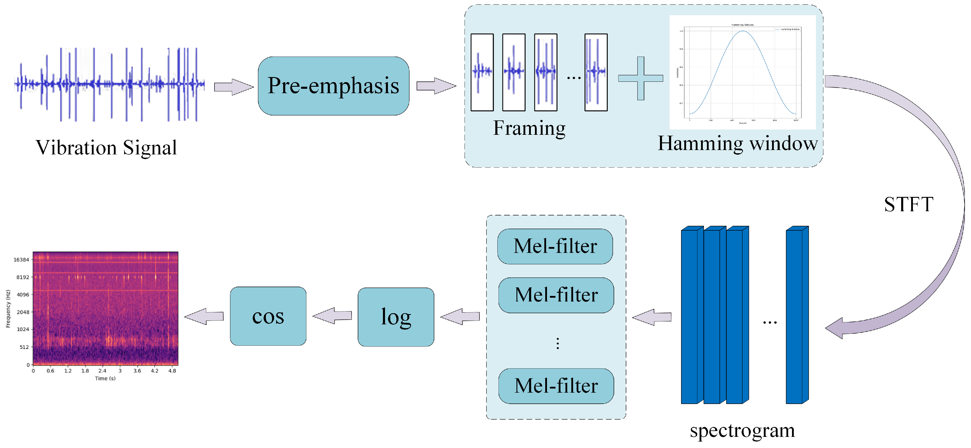
Figure 9 illustrates the MFCC feature extraction process, which includes the following steps: Firstly, the input vibration signal undergoes a pre-emphasis operation through a high-pass filter. This step enhances the high-frequency components of the signal while reducing the impact of low-frequency components, resulting in a more uniform spectral feature. Pre-emphasis is essentially a first-order difference, as shown in Equation (1). The signal is then divided into frames. The window size and frame shift are set to (25 ms, 10 ms), (50 ms, 25 ms), and (100 ms, 50 ms), respectively. A Hamming window is applied as the window function, as described in Equation (2). The Hamming window is a type of window function commonly used in time-domain signal processing, particularly in speech processing and spectral analysis. The purpose of applying a window is to reduce spectral leakage, allowing for a smoother transition at the edges of the signal and avoiding spectral distortion during framing. After windowing, multiple segments of the signal are considered stationary over short time intervals. The framed and windowed signal undergoes a short-time Fourier transform (STFT). The energy spectrum of each frame is calculated, taking the magnitude squared of the frequency spectrum of the speech signal (since frequency cannot be negative, and negative values should be discarded), with the number of sampling points set to 4410 (i.e., N = 4410) in the experiment, as shown in Equation (3). The energy spectrum is then passed through a Mel filter bank, converting the original signal from the frequency domain to the Mel scale. The conversion between the frequency and Mel scale is given by Equations (4) and (5). In the experiment, the number of filters in the Mel filter bank was set to 128. The Mel filter bank is a technique that maps frequency-domain information onto the Mel scale, making spectral analysis more aligned with human auditory perception. Finally, the logarithm of the filter output is taken to obtain the MFCC features.
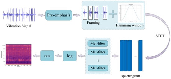
Figure 9.
Process of MFCC feature extraction.
Here, is the pre-emphasized signal, is the original input signal, and is the pre-emphasis coefficient, with a value of 0.97 used in the experiment. This value has been widely validated and is especially suitable for audio processing, speech recognition, and communication applications.
Here, , where N represents the length of the window function. And, represents the value of the Hamming window at the n-th point.
Here, represents the i-th audio signal segment before applying the short-time Fourier transform.
Here, m represents the Mel scale, and f is the frequency. This formula indicates that the frequency f is approximately linear in the low-frequency range, while in the high-frequency range, it follows a logarithmic growth. This aligns with the way the human ear perceives frequency.
4.2. Model Structure
Deep residual network-50 (ResNet50) is a residual network proposed by He et al. (2016) [45] to address the vanishing gradient problem in deep neural networks. By introducing “skip connections”, ResNet allows for the effective training of very deep networks without suffering from gradient decay. The core of this model is the residual module, which enables direct input transmission, allowing the network to learn deeper feature representations. It is widely used in tasks such as image classification and signal processing. The dense convolutional network (DenseNet), introduced by Huang et al. (2017) [46], is a densely connected convolutional neural network. Its defining characteristic is that the output of each layer is not only passed to the next layer but also directly connected to all subsequent layers. This structure promotes feature reuse, reduces the risk of overfitting, and enhances network efficiency without increasing the number of parameters. DenseNet is particularly suitable for processing high-dimensional data. The Inception network, initially proposed by Szegedy et al. (2015) [47], enhances the network’s expressive power by using parallel multi-scale convolutional kernels. By applying different sizes of convolutional filters within the same layer, the Inception network captures features at multiple scales, improving its ability to handle diverse features. This network is well suited for processing signals with complex characteristics. The Oxford Visual Geometry Group network (VGG), proposed by Simonyan and Zisserman (2015) [48], is known for its depth and simple structure. VGG uses small 3 × 3 convolutional kernels and enhances feature extraction by increasing the number of network layers. Although it has a large number of parameters, its hierarchical feature extraction approach performs exceptionally well in tasks such as image classification and pattern recognition. VGG is also suitable for processing structured data like vibration signals.
To accurately identify boring vibration signals within audio segments, this study proposes a novel deep neural network called BorerNet. The model utilizes MFCC features as input, which are processed through convolutional layers to learn and output recognition results. The concept of residual networks (ResNets) was introduced by He et al. in 2015 [45], with the fundamental idea that the true measured value equals the predicted value plus the residual. ResNets effectively address issues like network degradation and vanishing gradients that often occur during neural network training, which can lead to a decrease in recognition accuracy. BorerNet incorporates the residual learning mechanism to overcome the common problem of vanishing gradients in deep networks. This allows the network to be effectively trained and to capture complex patterns and subtle variations in audio signals. Experimental results indicate that BorerNet demonstrates high signal detection accuracy, particularly when handling audio data with significant noise interference, and it exhibits strong robustness and generalization capabilities.
The structure of BorerNet is illustrated in Figure 10. After standard processing, the extracted MFCC features of the pest’s boring vibration signals are fed into the BorerNet model. These features are first processed by 64 convolutional kernels with a size of (7, 7) and a stride of 2, which input the feature spectrum into different residual blocks. BorerNet consists of various residual blocks, where the signal is further processed. Finally, the output passes through an average pooling layer and a fully connected layer to determine whether the target pest’s boring vibration signal is present in the audio.
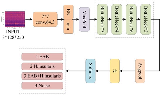
Figure 10.
The structure of BorerNet.
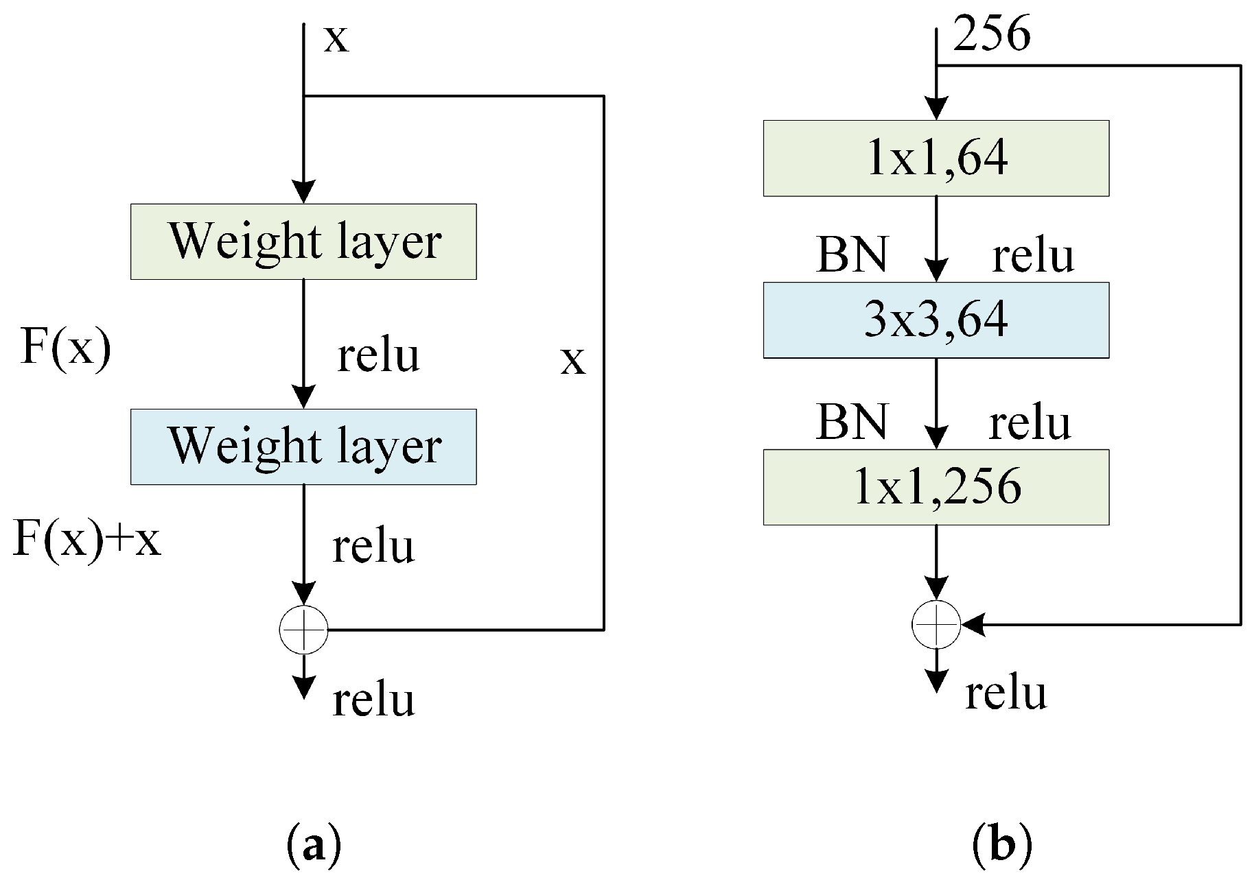
The residual block is the core building unit of the residual network (ResNet), designed to optimize the learning process of deep neural networks by calculating the residuals between the input and output. Specifically, a residual block emphasizes the difference between the input signal and the expected output. The structure of the residual block is illustrated in Figure 11a and described by Equation (6). In BorerNet, each residual block consists of two convolutional operations, along with a shortcut connection. The shortcut connection involves directly adding the input signal to the output signal, a design strategy that allows the network to focus on learning the difference, or residual function, between the input and output, rather than the entire mapping from input to output. The primary advantage of this approach is that, even if the learning process within the convolutional layers does not perform as expected, the network’s basic output can still retain the essential information from the input through the shortcut connection. BorerNet incorporates multiple residual structures, meaning the network only needs to learn corrections to the input, effectively mitigating errors in the identity mapping process. This helps address issues like gradient vanishing that can occur during training. Additionally, the shortcut connections reduce the number of parameters in the model, making the parameter count of the BorerNet model comparable to that of a traditional CNN with the same depth and structure, without adding extra computational overhead. This mechanism ensures that gradients can propagate backward to deeper layers, enhancing the overall training effectiveness and stability of the network. The innovation of this residual structure makes it easier to train deep neural networks and significantly improves their fitting capabilities, especially in handling complex pattern recognition and data modeling tasks.
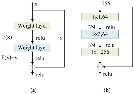
Figure 11.
(a) Residual block structure. (b) Residual structure using Bottleneck Blocks.
In this context, represents the residual function, where x is the input to the residual block, and is the output of the residual block. The Rectified Linear Unit (ReLU) is a commonly used activation function known for its simplicity in computation, non-linear characteristics in the positive range, and ability to mitigate the vanishing gradient problem. It is particularly prevalent in deep neural networks, such as convolutional neural networks (CNNs).
Due to the considerable depth of the BorerNet network, the model adopts an architecture known as the Bottleneck Block. The residual structure using Bottleneck Blocks is illustrated in Figure 11b, where the introduction of convolutions serves the purpose of reducing and restoring feature dimensions. The design of the Bottleneck Block aims to maintain the network’s depth and the information content of the output feature maps while reducing computational complexity and enhancing training efficiency. Each basic Bottleneck Block consists of three convolutional layers. The first is a convolution to reduce dimensionality, thereby decreasing the number of channels in the input feature maps and reducing the computational complexity of subsequent convolution operations. This is followed by a convolution for feature extraction. The final convolution is used for dimensionality restoration, bringing the number of channels back to its original size to ensure that the output matches the input dimensions. This bottleneck design significantly improves the efficiency and training performance of deep networks by reducing the computational load and parameters in the intermediate layers, making it particularly suitable for deep networks like BorerNet.
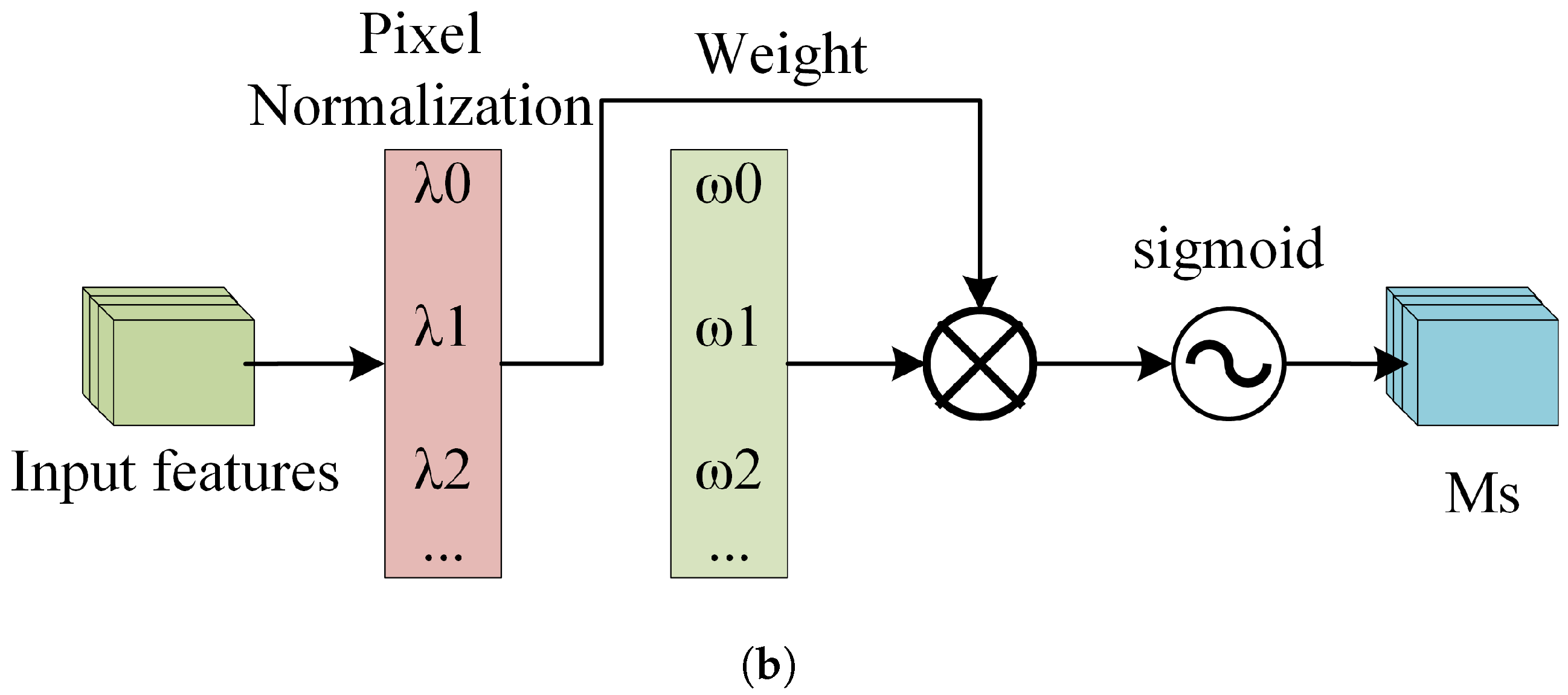
BorerNet introduces a normalization-based attention module (NAM), which suppresses insignificant features across both channel and spatial dimensions, making these weights computationally more efficient and enhancing the model’s focus. This improvement ultimately leads to increased recognition accuracy. Specifically, the NAM is embedded at the end of each residual block. This module uses the standard deviation to represent the importance of weights, thereby avoiding the complexity of adding fully connected layers and convolutional layers. This approach enhances recognition accuracy while ensuring the model remains lightweight. The NAM directly utilizes the scaling factors from the Batch Normalization (BN) layer to calculate attention weights. In doing so, the NAM efficiently adjusts the weights of various features, suppresses insignificant features, and enhances the extraction of significant ones [49].
Figure 12a depicts the channel attention submodule of the NAM, where represents the scaling factor for each channel, and is the channel attention weight calculated from , as shown in Equation (7). Figure 12b depicts the spatial attention submodule of the NAM, where represents the scaling factor for each pixel, and is the spatial attention weight calculated from , as shown in Equation (8).
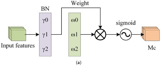

Figure 12.
The structure of the NAM. (a) The Channel Attention Mechanism. (b) The Spatial Attention Mechanism.
4.3. Lightweight Model Design
In practical application scenarios, it is necessary to deploy trained models onto mobile devices, where resources are often highly constrained, presenting a significant challenge. Therefore, lightweight optimization of the model can reduce system resource consumption, improve operational efficiency, lower power consumption, and enhance response speed [50]. In this study, ablation experiments were conducted, where non-essential parts of the model were removed, retaining only the core components. This initial compression of the model led to a significant reduction in the number of parameters while maintaining high recognition accuracy. Consequently, the model can operate in these environments with lower resource consumption and faster response times, thereby improving the overall experience and effectiveness in real-world applications.
5. Experimental Design
5.1. Experimental Environment
The environment of the experiment is shown in Table 3.
Table 3.
Specific experimental environment information.
5.2. Experimental Process
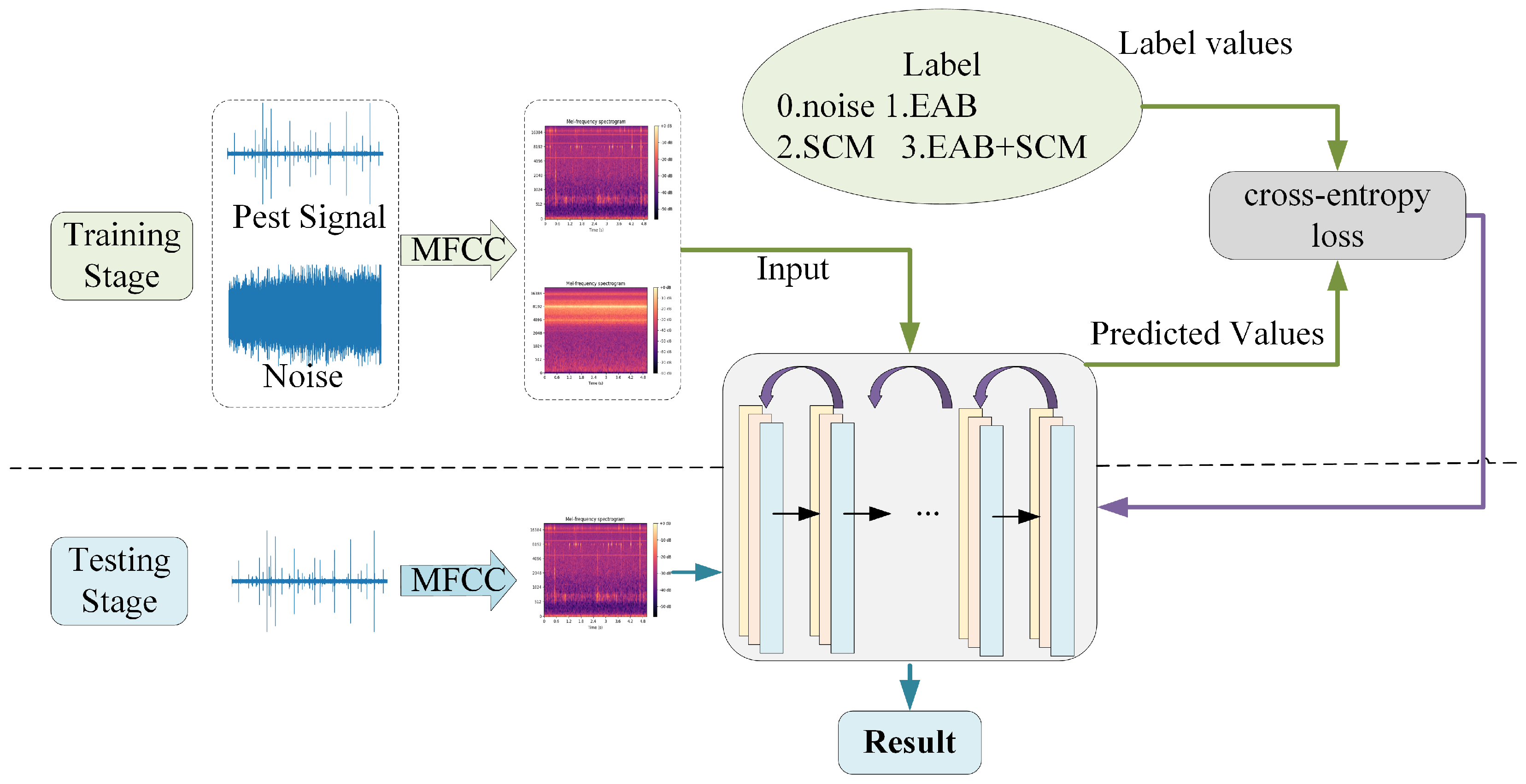
The speech signal is captured via a microphone and processed by an analog-to-digital converter (ADC) before being stored in digital form. Next, the signal undergoes preprocessing, which primarily includes denoising, data alignment, framing, and windowing. These steps are essential for minimizing background noise interference and preparing the data for subsequent feature extraction. In the feature extraction phase, the preprocessed speech signal is converted into features that can be understood by the model. In the experiment, MFCCs were used for spectral feature extraction. By applying short-time Fourier transform (STFT) analysis to the speech signal, frequency-domain features are extracted to capture phonetic characteristics and temporal variations within the speech signal. Once feature extraction is complete, these feature vectors are fed into the BorerNet model to generate predictions. These predictions, along with their corresponding true labels, are then input into the loss function. The model uses binary cross-entropy as the loss function, which is suitable for classification tasks, and calculates the loss value based on the difference between the predicted values and the true labels. The computed loss value reflects the accuracy of the model’s predictions, indicating the discrepancy between the model’s output and the actual results. To optimize the model’s performance, the calculated loss value is used to update the network’s parameters through backpropagation. This process adjusts the weights and biases within the network, enabling the model to progressively learn the features and patterns in the data, thus improving its ability to fit the training data. By iterating this process, the BorerNet model gradually enhances its feature extraction capabilities and ultimately becomes more accurate in performing the prediction task.
In the experiment, the batch size was set to 32, and the number of training iterations (epochs) was set to 20. Extensive experimentation demonstrated that this configuration ensures the model receives sufficient training to effectively learn and capture features from the audio data. Additionally, during the model training phase, the Adam algorithm was employed for efficient and robust parameter updates. The initial learning rate for the model was set to 0.0001, and it was adjusted to 0.1 times the original rate after every 5 epochs of training. The upper part of Figure 13 illustrates the training process of the model, where the arrows pointing to the right represent the forward propagation process, and the arrows pointing to the left represent the backpropagation process. The lower part of Figure 13 depicts the model’s validation process. In this stage, preprocessed audio segments are input into the model, which loads the parameter set that performed optimally during training, thereby enhancing its predictive capabilities. The model then performs computations and outputs predictions, determining whether the audio segments contain signals of pest boring activity and identifying the type of pest present.
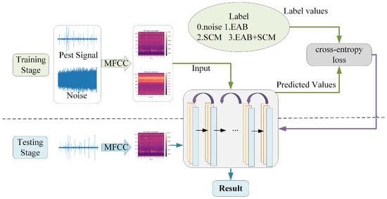
Figure 13.
Flowchart of model training and testing.
5.3. Evaluation Index
In deep learning classification tasks, the evaluation metrics for model performance are crucial as they directly influence the understanding of the model’s practical effectiveness and the formulation of optimization strategies. Among these metrics, accuracy and F1 score are two widely used indicators for assessing the performance of classification models. Each of these metrics has distinct characteristics, providing deep insights into the model’s performance from different perspectives. In this study, which explores the recognition of boring vibration signals, a typical classification task, both accuracy and F1 score were employed as key metrics to comprehensively evaluate the performance of the proposed model. This choice not only provides a holistic view of the model’s overall performance but also reveals its ability to correctly identify samples across different categories. Additionally, these metrics allow for a comparative analysis between the proposed model and other classical models. The experimental results demonstrate that BorerNet significantly outperforms the comparison models in terms of both accuracy and F1 score, indicating its superior recognition performance and generalization ability in detecting boring vibration signals. This comparison further validates the advantages of BorerNet in classification tasks, offering strong support for its application in real-world scenarios.
1. Accuracy: Accuracy is the ratio of the number of correctly predicted samples to the total number of samples. It is an intuitive and widely used performance metric, particularly effective in classification tasks where the sample distribution is relatively balanced. The calculation of accuracy is shown in Equation (9):
In this context, TP (true positive) represents the number of instances where the model correctly predicts the positive class, TN (true negative) represents the number of instances where the model correctly predicts the negative class, FP (false positive) represents the number of instances where the model incorrectly predicts the positive class, and FN (false negative) represents the number of instances where the model incorrectly predicts the negative class.
2. F1 Score: The F1 score is the harmonic mean of precision and recall, effectively balancing the trade-off between these two metrics. It is particularly useful in situations where the class distribution is imbalanced, as it combines both precision and recall to provide a holistic view of the model’s performance in identifying both positive and negative classes. The F1 score is calculated using the following Equations (10)–(12):
where TP represents the number of true positives, FP represents the number of false positives, and FN represents the number of false negatives.
5.4. Results and Analysis
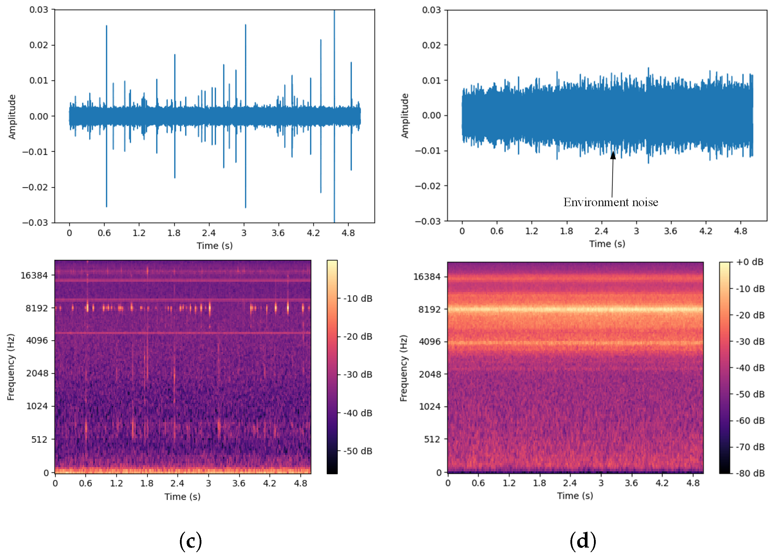
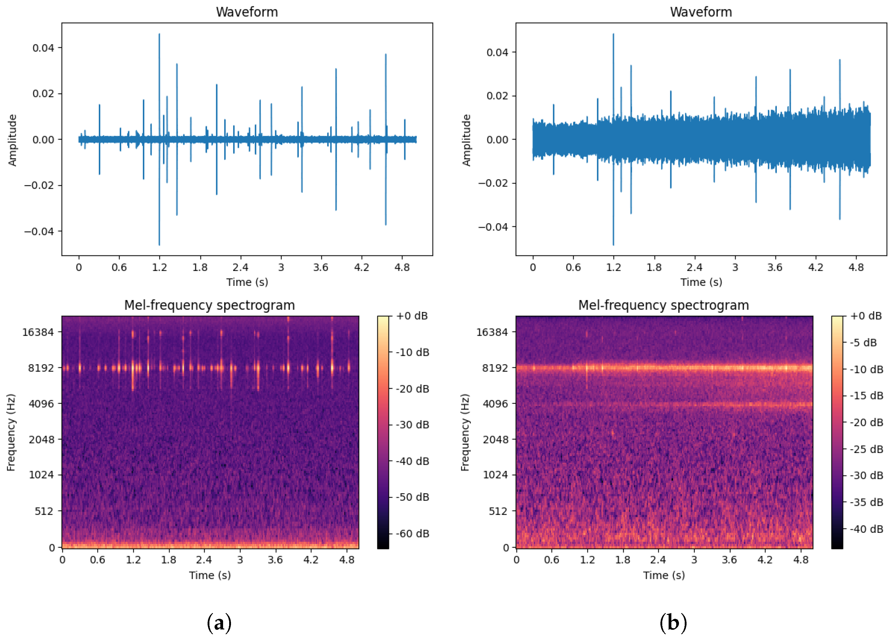
To more fully extract signal features, this paper selected pure boring vibration signals collected in a soundproof room as the training set while using signals from real outdoor environments as the test set. The waveforms and spectrograms of both noisy and pure EAB boring vibration signals are shown in Figure 14.
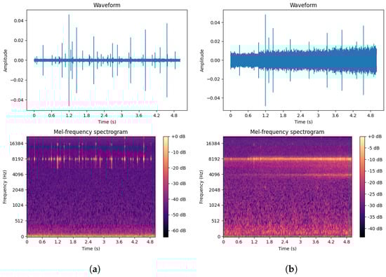
Figure 14.
(a) Pure EAB boring vibration signal in a soundproof room. (b) Noisy EAB boring vibration signal in a real environment.
Figure 15 shows the loss curve during the model training process. The trend of the curve indicates that the loss value decreases rapidly in the early stages of training and then levels off, eventually reaching a very low and convergent state in the subsequent epochs. This suggests that the model quickly learns important features during training, and as training progresses, the loss value continually decreases, approaching zero, indicating that training is effective and the model achieves a high level of accuracy.
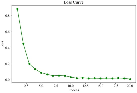
Figure 15.
Loss curve.
To validate the performance of the BorerNet model, the paper designed comparative experiments with several well-established classic networks. Generally speaking, deeper and more complex neural networks tend to capture and solve more intricate problems. However, in specific classification tasks, the complexity of the network does not always correlate positively with performance. In some cases, simpler network architectures might actually provide higher recognition accuracy. Therefore, this research not only evaluates the performance of the BorerNet model but also includes comparative experiments with ResNet50, DenseNet, Inception, and VGG networks, using the same dataset and evaluation metrics.
Table 4 displays the performance of five models, with BorerNet showing the best results, achieving an accuracy of 96.67% and an F1 score of 0.95, demonstrating exceptional classification capability. Following closely is ResNet50, which achieved an accuracy of 93.67% and an F1 score of 0.93, also exhibiting strong performance. DenseNet performed reasonably well, albeit with a slightly lower accuracy of 88.33% and an F1 score of 0.90. Inception V3 and VGG showed lower performance, with accuracies of 77.67% and 72.33% and F1 scores of 0.79 and 0.72, indicating their limitations in high-demand tasks. This suggests that BorerNet has a greater capability to process complex signal features and handle noise interference effectively. The model’s outstanding performance indicates its potential to provide more reliable and accurate recognition results in real-world applications, which is crucial for improving the efficiency and accuracy of pest detection.
Table 4.
Experimental results.
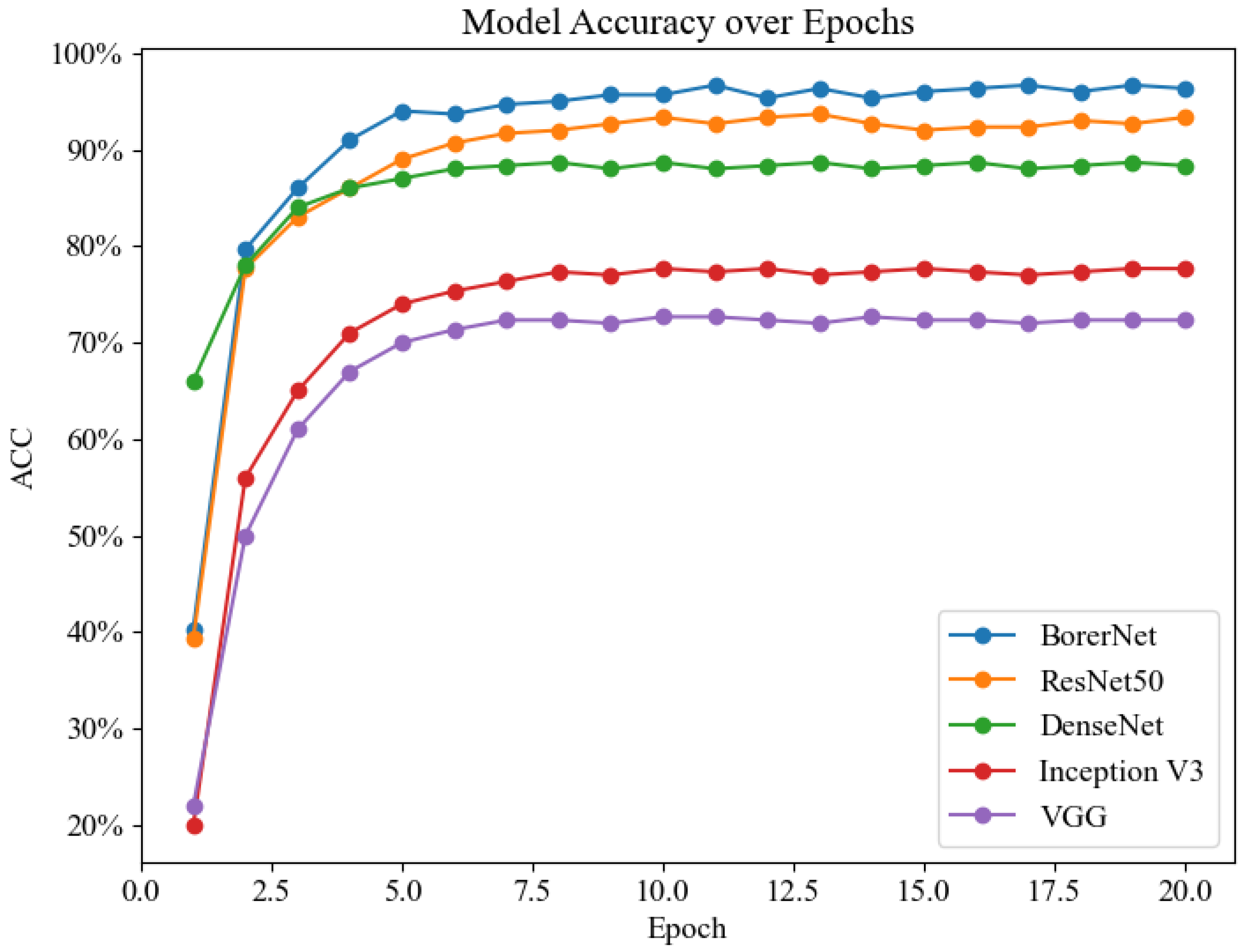
Figure 16 presents the line chart of recognition accuracy for the five models. Overall, the recognition accuracy of these models shows a significant increase during the first five epochs, after which it stabilizes at a relatively high level. Among them, BorerNet’s accuracy is noticeably higher than that of ResNet50, and both models maintain a recognition accuracy of over 90%. In contrast, the recognition abilities of the Inception and VGG models are significantly lower than the other three models. This result underscores the rationale behind the model selection in this experiment and further demonstrates that the optimizations applied to the BorerNet model give it an advantage in feature extraction and recognition capability.
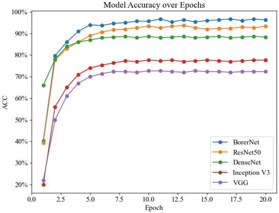
Figure 16.
Recognition accuracy line chart.
The confusion matrix is shown in Figure 17, where deeper colors represent higher values. By analyzing the confusion matrix, it is evident that the most prominent misclassification occurs when the model confuses environmental noise and EAB borer vibration signals with SCM borer vibration signals. This misclassification might be attributed to the indistinct features of certain audio segments, which lead to difficulties in the model’s ability to differentiate between them. However, the majority of signal categories are correctly classified, and the confusion matrix overall demonstrates BorerNet’s superior recognition performance in most real-world scenarios.
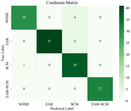
Figure 17.
Confusion matrix.
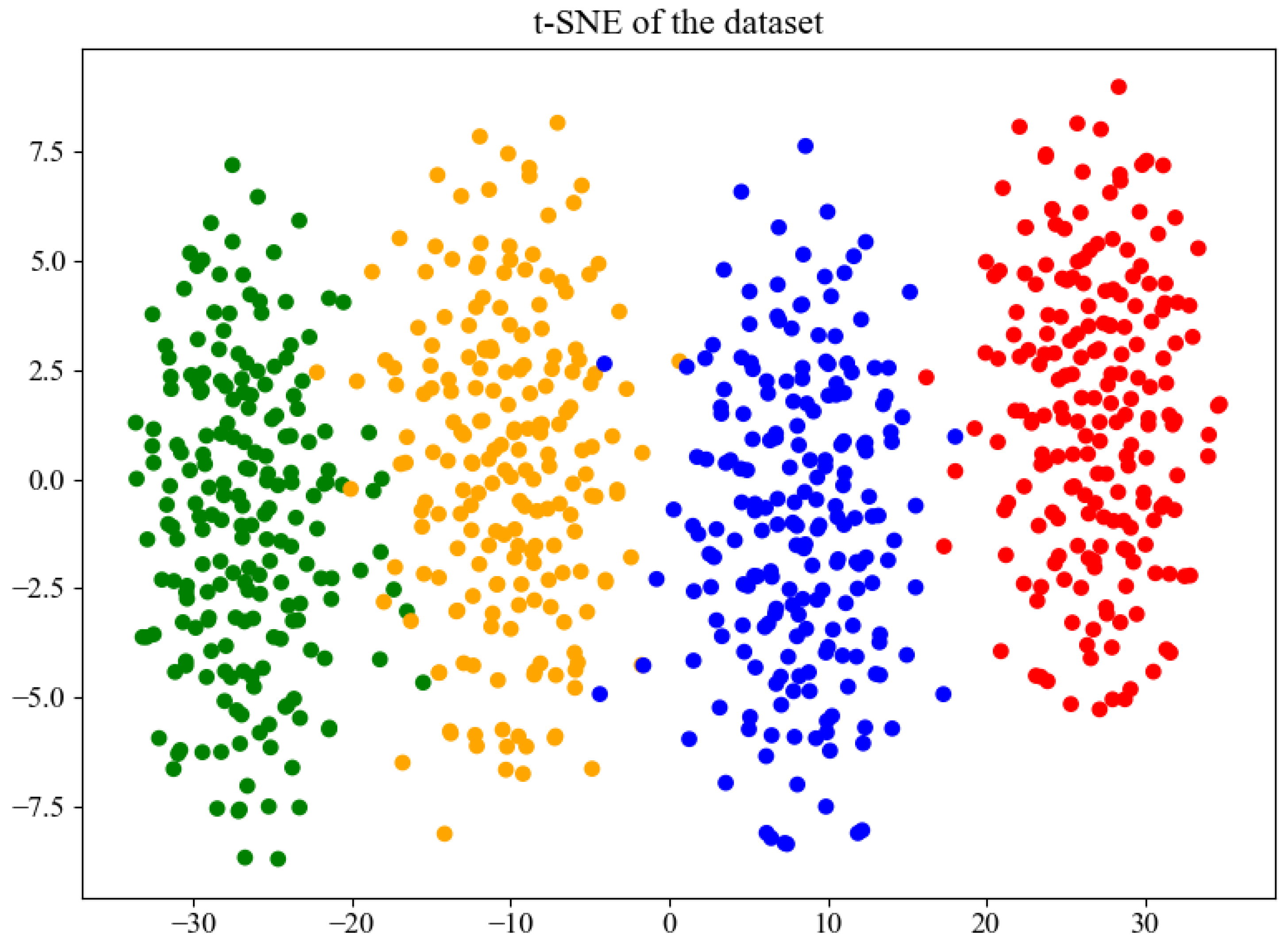
The t-distributed Stochastic Neighbor Embedding (t-SNE) algorithm was employed to visualize the features learned by the BorerNet model. The visualization includes the EAB (green), the SCM (orange), noise (blue), and mixed signals of the EAB and SCM (red). The results are shown in Figure 18. As depicted in the figure, BorerNet effectively distinguishes the characteristics of the three different boring vibration signals and noise. There is a slight overlap between the vibration signals of the SCM and those of the noise and EAB signals, which is consistent with the results observed in the confusion matrix.
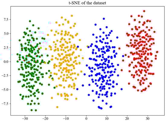
Figure 18.
Feature distribution visualized using t-SNE.
6. Discussion
We found very few trees infected with fungi during the data collection process, and we selected trees that did not have infections. Fungal infections that cause cavities in the tree trunk or affect the softness of the trunk’s texture will only impact the amplitude and phase of the collected signal, without affecting the signal’s frequency. The frequency of the signal is determined solely by the sound source, which, in this case, is the pest activity. Since this study identifies pests based on the frequency of the boring vibration signals, such factors will not affect the experimental results. For the same reason, the development and morphology of the larvae did not affect the results.
This paper utilizes deep learning methods for the classification of wood-boring pests using drilling vibration signals as input, which offers significant advantages. Firstly, deep learning models can automatically extract complex features from large amounts of vibration data, improving classification accuracy and demonstrating clear superiority in data processing speed and efficiency compared to traditional methods. Secondly, this approach enables real-time monitoring, allowing for the immediate detection and classification of pest activity and a rapid response to threats. Additionally, automation reduces the need for manual intervention, lowering costs, and the model’s strong adaptability ensures high performance across different environments.
Although this study has achieved significant results, there are still areas worth further exploration. The current research primarily focuses on identifying larvae of two target pest species. Future work could extend to a broader range of pest species. The model developed in this paper is also applicable to the identification of other wood-boring pests, but it requires prior data collection for training. Preliminary research has revealed that many white ash trees in urban areas are infected by the EAB and SCM, while a small number of white ash trees are affected by Click beetle larvae (Coleoptera: Elateridae). However, due to their low numbers, data collection for this pest is challenging, and there is no large-scale outbreak in the area, making the threat less apparent. Exploring advanced model compression techniques to further reduce model size and enhance its performance on ultra-low-power devices is also a potential avenue. Additionally, integrating Internet of Things (IoT) technology to develop real-time monitoring and early warning systems could enable continuous monitoring and timely alerts for pest activity. With ongoing research and innovation, the technical solutions proposed in this study are expected to find widespread application in the future, providing robust technological support for the control of wood-boring pests. In addition, there are many figures in this paper, and we have indexed them for easy reading in the Appendix A.
7. Conclusions
This paper presents a pest identification model based on deep learning to achieve the automated identification of pests, using the EAB and SCM as examples. The original data used in this study were collected using custom-developed equipment, capturing signals from both real-world environments and within a soundproof chamber. The raw signals underwent preprocessing, and simulated signals were synthesized using computer technology to successfully build the experimental dataset. The method proposed in this paper enables automated monitoring and classification of wood-boring pests with high efficiency and low cost. Experiments have demonstrated that the model not only achieves high recognition accuracy but also exhibits good generalization ability and robustness. The advancements achieved in this study represent a breakthrough in pest monitoring and recognition technologies, providing an effective tool for forest pest management and offering critical technical support for the sustainable development of forestry and urban ecosystems, as well as for the protection of global biodiversity.
Author Contributions
Conceptualization, X.Z. and J.L.; methodology, X.Z.; software, X.Z.; validation, X.Z. and J.L.; formal analysis, X.Z.; investigation, X.Z.; resources, X.Z.; data curation, J.L. and F.Y.; writing—original draft, X.Z.; writing—review and editing, X.Z., J.L. and F.Y.; visualization, X.L. and M.J.; supervision, X.L. and F.Y.; project administration, M.J. and F.Y.; funding acquisition, F.Y. All authors have read and agreed to the published version of the manuscript.
Funding
This research was supported by the National Natural Science Foundation of China, grant number 32071775. This research was supported by the National Key R&D Program of China, grant number 2022YFF1302700. This research was supported by The Emergency Open Competition Project of National Forestry and Grassland Administration (202303). This research was supported by the Outstanding Youth Team Project of Central Universities, grant number QNTD202308.
Institutional Review Board Statement
Not applicable.
Informed Consent Statement
Not applicable.
Data Availability Statement
The data presented in this study are available on request from the corresponding author.
Conflicts of Interest
The authors declare no conflicts of interest.
Appendix A. Insect Hazards and Data Collection Table
| Figure | Caption | Page |
| Figure 1a | Galleries created by EAB due to prolonged feeding. | 3 |
| Figure 1b | D-shaped exit hole left after EAB emerges. | 3 |
| Figure 2a | Boreholes observed after cutting open the tree trunk. | 4 |
| Figure 2b | The pupal cases and exit holes left on the tree trunk surface after SCM emerges. | 4 |
| Figure 3a | Self-developed piezoelectric sensor. | 7 |
| Figure 3b | Multi-channel signal acquisition device. | 7 |
| Figure 4a | Weijiadian Village. | 8 |
| Figure 4b | Xianggezhuang Village | 8 |
| Figure 5a | Embedding the probe into the tree trunk using a power drill. | 9 |
| Figure 5b | Monitoring larval activity. | 9 |
| Figure 5c | Capturing signals using a piezoelectric sensor. | 9 |
| Figure 5d | Collecting signals using a multi-channel acquisition device. | 9 |
| Figure 6a | Cross-sections of tree trunks infested with EAB. | 10 |
| Figure 6b | Monitoring boring vibration signals within the tree trunk. | 10 |
| Figure 6c | Collecting EAB boring vibration signals in a soundproof room using a multi-channel acquisition device. | 10 |
| Figure 6d | Counting the number of larvae within the tree trunks. | 10 |
References
- Pimm, S.L.; Jenkins, C.N.; Abell, R.; Brooks, T.M.; Gittleman, J.L.; Joppa, L.N.; Raven, P.H.; Roberts, C.M.; Sexton, J.O. The biodiversity of species and their rates of extinction, distribution, and protection. Science 2014, 344, 1246752. [Google Scholar] [CrossRef] [PubMed]
- Boyd, I.L.; Freer-Smith, P.H.; Gilligan, C.A.; Godfray, H.C.J. The consequence of tree pests and diseases for ecosystem services. Science 2013, 342, 1235773. [Google Scholar] [CrossRef]
- Nesbitt, L.; Meitner, M.J.; Girling, C.; Sheppard, S.R.; Lu, Y. Who has access to urban vegetation? A spatial analysis of distributional green equity in 10 US cities. Landsc. Urban Plan. 2019, 181, 51–79. [Google Scholar] [CrossRef]
- Orlova-Bienkowskaja, M.J.; Drogvalenko, A.N.; Zabaluev, I.A.; Sazhnev, A.S.; Peregudova, E.Y.; Mazurov, S.G.; Komarov, E.V.; Struchaev, V.V.; Martynov, V.V.; Nikulina, T.V.; et al. Current range of Agrilus planipennis Fairmaire, an alien pest of ash trees, in European Russia and Ukraine. Ann. For. Sci. 2020, 77, 1–14. [Google Scholar] [CrossRef]
- Zhang, Q.H.; Schlyter, F. Olfactory recognition and behavioural avoidance of angiosperm nonhost volatiles by conifer-inhabiting bark beetles. Agric. For. Entomol. 2004, 6, 1–20. [Google Scholar] [CrossRef]
- Timms, L.L.; Smith, S.M.; De Groot, P. Patterns in the within-tree distribution of the emerald ash borer Agrilus planipennis (Fairmaire) in young, green-ash plantations of south-western Ontario, Canada. Agric. For. Entomol. 2006, 8, 313–321. [Google Scholar] [CrossRef]
- Cappaert, D.; McCullough, D.G.; Poland, T.M.; Siegert, N.W. Emerald ash borer in North America: A research and regulatory challenge. Am. Entomol. 2005, 51, 152. [Google Scholar] [CrossRef]
- Aukema, J.E.; McCullough, D.G.; Von Holle, B.; Liebhold, A.M.; Britton, K.; Frankel, S.J. Historical accumulation of nonindigenous forest pests in the continental United States. BioScience 2010, 60, 886–897. [Google Scholar] [CrossRef]
- Lovett, G.M.; Canham, C.D.; Arthur, M.A.; Weathers, K.C.; Fitzhugh, R.D. Forest ecosystem responses to exotic pests and pathogens in eastern North America. BioScience 2006, 56, 395–405. [Google Scholar] [CrossRef]
- Herms, D.A.; McCullough, D.G. Emerald ash borer invasion of North America: History, biology, ecology, impacts, and management. Annu. Rev. Entomol. 2014, 59, 13–30. [Google Scholar] [CrossRef]
- Poland, T.M.; McCullough, D.G. Emerald ash borer: Invasion of the urban forest and the threat to North America’s ash resource. J. For. 2006, 104, 118–124. [Google Scholar] [CrossRef]
- Silk, P.J.; Ryall, K.; Roscoe, L. Emerald ash borer, Agrilus planipennis (Coleoptera: Buprestidae), detection and monitoring in Canada. For. Int. J. For. Res. 2020, 93, 273–279. [Google Scholar] [CrossRef]
- Yang, Z.Q.; Wang, X.Y.; Zhang, Y.N. Recent advances in biological control of important native and invasive forest pests in China. Biol. Control 2014, 68, 117–128. [Google Scholar] [CrossRef]
- Desneux, N.; Decourtye, A.; Delpuech, J.M. The sublethal effects of pesticides on beneficial arthropods. Annu. Rev. Entomol. 2007, 52, 81–106. [Google Scholar] [CrossRef] [PubMed]
- Duan, J.J.; Crandall, R.S.; Grosman, D.M.; Schmude, J.M.; Quinn, N.; Chandler, J.L.; Elkinton, J.S. Effects of emamectin benzoate trunk injections on protection of neighboring ash trees against emerald ash borer (Coleoptera: Buprestidae) and on established biological control agents. J. Econ. Entomol. 2023, 116, 848–854. [Google Scholar] [CrossRef]
- Herms, D.A.; McCullough, D.G.; Smitley, D.R.; Sadof, C.S.; Williamson, R.C.; Nixon, P.L. Insecticide options for protecting ash trees from emerald ash borer. North Cent. IPM Cent. Bull. 2009, 12, 1–24. [Google Scholar]
- Quinn, N.F.; Petrice, T.R.; Schmude, J.M.; Poland, T.M.; Bauer, L.S.; Rutlege, C.E.; Van Driesche, R.G.; Elkinton, J.S.; Duan, J.J. Postrelease assessment of Oobius agrili (Hymenoptera: Encyrtidae) establishment and persistence in Michigan and the Northeastern United States. J. Econ. Entomol. 2023, 116, 1165–1170. [Google Scholar] [CrossRef]
- Gullan, P.J.; Cranston, P.S. The Insects: An Outline of Entomology; John Wiley & Sons: New York, NY, USA, 2014. [Google Scholar]
- Abbott, D. The Apple Tree: Physiology and Management; Grower Books: Berlin, Germany, 1984. [Google Scholar]
- Nowak, D.J.; Pasek, J.E.; Sequeira, R.A.; Crane, D.E.; Mastro, V.C. Potential effect of Anoplophora glabripennis (Coleoptera: Cerambycidae) on urban trees in the United States. J. Econ. Entomol. 2001, 94, 116–122. [Google Scholar] [CrossRef]
- Smith, M.T.; Tobin, P.C.; Bancroft, J.; Li, G.; Gao, R. Dispersal and spatiotemporal dynamics of Asian longhorned beetle (Coleoptera: Cerambycidae) in China. Environ. Entomol. 2004, 33, 435–442. [Google Scholar] [CrossRef]
- Zhang, Y. A Brief Discussion on the Occurrence and Control of the Little Leaf Borer Moth. Fruit Grow. Friend 2024, 21, 126–128. [Google Scholar]
- Kogan, M. Integrated pest management: Historical perspectives and contemporary developments. Annu. Rev. Entomol. 1998, 43, 243–270. [Google Scholar] [CrossRef] [PubMed]
- Pedigo, L.P.; Rice, M.E.; Krell, R.K. Entomology and Pest Management; Waveland Press: Long Grove, IL, USA, 2021. [Google Scholar]
- Kovacs, K.F.; Haight, R.G.; McCullough, D.G.; Mercader, R.J.; Siegert, N.W.; Liebhold, A.M. Cost of potential emerald ash borer damage in US communities, 2009–2019. Ecol. Econ. 2010, 69, 569–578. [Google Scholar] [CrossRef]
- Mankin, R.W.; Hagstrum, D.W.; Smith, M.T.; Roda, A.; Kairo, M.T. Perspective and promise: A century of insect acoustic detection and monitoring. Am. Entomol. 2011, 57, 30–44. [Google Scholar] [CrossRef]
- Farr, I.; Chesmore, D. Automated bioacoustic detection and identification of wood-boring insects for quarantine screening and insect ecology. Proc. Inst. Acoust. 2007, 29, 201–208. [Google Scholar]
- Schnitzler, H.U.; Kalko, E.K. Echolocation by insect-eating bats: We define four distinct functional groups of bats and find differences in signal structure that correlate with the typical echolocation tasks faced by each group. Bioscience 2001, 51, 557–569. [Google Scholar] [CrossRef]
- Yazgaç, B.G.; Kırcı, M.; Kıvan, M. Detection of sunn pests using sound signal processing methods. In Proceedings of the 2016 Fifth International Conference on Agro-Geoinformatics (Agro-Geoinformatics), Tianjin, China, 18–20 July 2016; pp. 1–6. [Google Scholar]
- Njoroge, A.; Affognon, H.; Mutungi, C.; Rohde, B.; Richter, U.; Hensel, O.; Mankin, R. Frequency and time pattern differences in acoustic signals produced by Prostephanus truncatus (Horn) (Coleoptera: Bostrichidae) and Sitophilus zeamais (Motschulsky) (Coleoptera: Curculionidae) in stored maize. J. Stored Prod. Res. 2016, 69, 31–40. [Google Scholar] [CrossRef]
- Jalinas, J.; Güerri-Agulló, B.; Mankin, R.; Lopez-Follana, R.; Lopez-Llorca, L.V. Acoustic assessment of Beauveria bassiana (Hypocreales: Clavicipitaceae) effects on Rhynchophorus ferrugineus (Coleoptera: Dryophthoridae) larval activity and mortality. J. Econ. Entomol. 2015, 108, 444–453. [Google Scholar] [CrossRef]
- Herrick, N.J.; Mankin, R. Acoustical detection of early instar Rhynchophorus ferrugineus (Coleoptera: Curculionidae) in Canary Island date palm, Phoenix canariensis (Arecales: Arecaceae). Fla. Entomol. 2012, 95, 983–990. [Google Scholar] [CrossRef]
- Mankin, R.; Al-Ayedh, H.; Aldryhim, Y.; Rohde, B. Acoustic detection of Rhynchophorus ferrugineus (Coleoptera: Dryophthoridae) and Oryctes elegans (Coleoptera: Scarabaeidae) in Phoenix dactylifera (Arecales: Arecacae) trees and offshoots in Saudi Arabian orchards. J. Econ. Entomol. 2016, 109, 622–628. [Google Scholar] [CrossRef]
- Mankin, R.; Burman, H.; Menocal, O.; Carrillo, D. Acoustic detection of Mallodon dasystomus (Coleoptera: Cerambycidae) in Persea americana (Laurales: Lauraceae) branch stumps. Fla. Entomol. 2018, 101, 321–323. [Google Scholar] [CrossRef]
- Eliopoulos, P.A.; Potamitis, I.; Kontodimas, D.C. Estimation of population density of stored grain pests via bioacoustic detection. Crop Prot. 2016, 85, 71–78. [Google Scholar] [CrossRef]
- Mankin, R.; Hagstrum, D.; Guo, M.; Eliopoulos, P.; Njoroge, A. Automated applications of acoustics for stored product insect detection, monitoring, and management. Insects 2021, 12, 259. [Google Scholar] [CrossRef] [PubMed]
- Luo, C.Y.; Pearson, P.; Xu, G.; Rich, S.M. A computer vision-based approach for tick identification using deep learning models. Insects 2022, 13, 116. [Google Scholar] [CrossRef]
- Zhu, L.; Zhang, Z. Automatic recognition of insect sounds using MFCC and GMM. Acta Entomol. Sin. 2012, 55, 466–471. [Google Scholar]
- Sun, Y.; Tuo, X.; Jiang, Q.; Zhang, H.; Chen, Z.; Zong, S.; Luo, Y. Drilling Vibration Identification Technique of Two Pest Based on Lightweight Neural Networks; The Chinese Society of Forestry: Beijing, China, 2020. [Google Scholar]
- Zhang, H.; Li, J.; Cai, G.; Chen, Z.; Zhang, H. A CNN-based method for enhancing boring vibration with time-domain convolution-augmented transformer. Insects 2023, 14, 631. [Google Scholar] [CrossRef]
- Jiang, W.; Chen, Z.; Zhang, H. A Time-Frequency Domain Mixed Attention-Based Approach for Classifying Wood-Boring Insect Feeding Vibration Signals Using a Deep Learning Model. Insects 2024, 15, 282. [Google Scholar] [CrossRef]
- Dong, Q.; Sun, L.; Han, T.; Cai, M.; Gao, C. PestLite: A novel YOLO-based deep learning technique for crop pest detection. Agriculture 2024, 14, 228. [Google Scholar] [CrossRef]
- Tang, Z.; Lu, J.; Chen, Z.; Qi, F.; Zhang, L. Improved Pest-YOLO: Real-time pest detection based on efficient channel attention mechanism and transformer encoder. Ecol. Inform. 2023, 78, 102340. [Google Scholar] [CrossRef]
- Wang, C.; Wang, P.; Xuan, Y.; Yang, L.; Zhang, J.; He, M.; Wang, S. Investigation on the Occurrence and Damage of the White Wax Scale, a Pest of Populus tomentosa in Karamay City. Plant Prot. 2023, 49, 304–310. [Google Scholar]
- He, K.; Zhang, X.; Ren, S.; Sun, J. Deep residual learning for image recognition. In Proceedings of the IEEE Conference on Computer Vision and Pattern Recognition, Las Vegas, NV, USA, 27–30 June 2016; pp. 770–778. [Google Scholar]
- Huang, G.; Liu, Z.; Van Der Maaten, L.; Weinberger, K.Q. Densely connected convolutional networks. In Proceedings of the IEEE Conference on Computer Vision and Pattern Recognition, Honolulu, HI, USA, 21–26 July 2017; pp. 4700–4708. [Google Scholar]
- Szegedy, C.; Liu, W.; Jia, Y.; Sermanet, P.; Reed, S.; Anguelov, D.; Erhan, D.; Vanhoucke, V.; Rabinovich, A. Going deeper with convolutions. In Proceedings of the IEEE Conference on Computer Vision and Pattern Recognition, Boston, MA, USA, 7–12 June 2015; pp. 1–9. [Google Scholar]
- Simonyan, K.; Zisserman, A. Very deep convolutional networks for large-scale image recognition. arXiv 2014, arXiv:1409.1556. [Google Scholar]
- Liu, Y.; Shao, Z.; Teng, Y.; Hoffmann, N. NAM: Normalization-based attention module. arXiv 2021, arXiv:2111.12419. [Google Scholar]
- Jacob, B.; Kligys, S.; Chen, B.; Zhu, M.; Tang, M.; Howard, A.; Adam, H.; Kalenichenko, D. Quantization and training of neural networks for efficient integer-arithmetic-only inference. In Proceedings of the IEEE Conference on Computer Vision and Pattern Recognition, Salt Lake City, UT, USA, 18–23 June 2018; pp. 2704–2713. [Google Scholar]


Disclaimer/Publisher’s Note: The statements, opinions and data contained in all publications are solely those of the individual author(s) and contributor(s) and not of MDPI and/or the editor(s). MDPI and/or the editor(s) disclaim responsibility for any injury to people or property resulting from any ideas, methods, instructions or products referred to in the content. |
© 2024 by the authors. Licensee MDPI, Basel, Switzerland. This article is an open access article distributed under the terms and conditions of the Creative Commons Attribution (CC BY) license (https://creativecommons.org/licenses/by/4.0/).