Article

Analysis of the Effects of Different Nitrogen Application Levels on the Growth of Castanopsis hystrix from the Perspective of Three-Dimensional Reconstruction

1
Institute of Forest Resource Information Techniques, Chinese Academy of Forestry, Beijing 100091, China
2
Key Laboratory of Forest Management and Growth Modelling, National Forestry and Grassland Administration, Beijing 100091, China
*
Author to whom correspondence should be addressed.
Forests 2024, 15(9), 1558; https://doi.org/10.3390/f15091558
Submission received: 30 July 2024 / Revised: 22 August 2024 / Accepted: 2 September 2024 / Published: 4 September 2024

Abstract

:
Monitoring tree growth helps operators better understand the growth mechanism of trees and the health status of trees and to formulate more effective management measures. Computer vision technology can quickly restore the three-dimensional geometric structure of trees from two-dimensional images of trees, playing a huge role in planning and managing tree growth. This study used binocular reconstruction technology to measure the height, canopy width, and ground diameter of Castanopsis hystrix and compared the growth differences under different nitrogen levels. In this research, we proposed a wavelet exponential decay thresholding method for image denoising. At the same time, based on the traditional semi-global matching (SGM) algorithm, a cost search direction is added, and a multi-line scanning semi-global matching (MLC-SGM) algorithm for stereo matching is proposed. The results show that the wavelet exponential attenuation threshold method can effectively remove random noise in red cone images, and the denoising effect is better than the traditional hard-threshold and soft-threshold denoising methods. The disparity images produced by the MLC-SGM algorithm have better disparity continuity and noise suppression than those produced by the SGM algorithm, with more minor measurement errors for C. hystrix growth factors. Medium nitrogen fertilization significantly promotes the height, canopy width, and ground diameter growth of C. hystrix. However, excessive fertilization can diminish this effect. Compared to tree height, excessive fertilization has a more pronounced impact on canopy width and ground diameter growth.

1. Introduction

Collecting forest tree data is the basis of the forest resource survey. The measurement accuracy of individual tree attributes, such as tree height and crown width, directly affects the estimation results of forest information [1]. However, the traditional way of measuring forest information is mainly manual, which is low in automation and time-consuming and laborious [2]. Therefore, it is impossible for traditional measurement methods to continuously measure multiple factors in the field, making it difficult for forestry workers to fully grasp the growth mechanism of trees and make them unable to manage and protect trees in real time. If we can accurately obtain information on trees and determine their growth status with the help of efficient, intelligent sensing equipment, we can realize the dynamic monitoring of tree growth and promote its healthy growth [3,4].
Among many types of sensor data, images have the characteristics of high spatial resolution and high temporal resolution, carry a large amount of information, and are the main body of sensor data [5]. At present, image-based two-dimensional tree-phenotyping methods have been widely used, but their most significant disadvantage is that they cannot obtain three-dimensional spatial information of trees [6]. Passive reconstruction of tree phenotypes through stereo vision technology can effectively solve this problem, that is, applying the camera imaging principle to reversely restore the three-dimensional structure of trees from two-dimensional images, thereby obtaining more traits [7,8,9]. In addition, ground-based laser radar [10,11], laser scanners [12,13], ultrasonic sensors [14,15], optical sensors [16], and high-resolution radar images [17] are also used to accurately measure the 3D geometry of trees. However, the equipment required for ground-based laser radar, laser sensors, and high-resolution radar images is expensive and complex to operate. The measurement accuracy of ultrasonic sensors and optical sensors is greatly affected by the environment and has a small scope of application. In contrast, stereo vision technology is not only low-cost but also easy to operate, providing the conditions for the accurate acquisition of the three-dimensional structural information of trees.
Recently, researchers have applied stereoscopic vision technology to the study of plant phenotypic structures and geometric parameters. For example, a study used three digital cameras to capture multi-view images of wheat regularly, and by reconstructing a 3D model of the wheat, they extracted growth parameters, such as the number of leaves, plant height, and leaf length, thereby detecting early growth trends of the wheat [18]. Another research study used ten calibrated cameras to construct a 3D data-acquisition device, from which a 3D model of tomatoes was derived to identify leaves and measure the length, width, and area of individual leaves [19]. This technique was also applied to the acquisition of depth information for date trees; researchers achieved non-destructive measurement of the geometric parameters of the date trees by capturing a sequence of multi-angle images [20]. Multi-camera and multi-view reconstruction can provide high-precision depth information, but the system complexity is high, and the reconstruction efficiency is low [21]. In contrast, when using binocular vision to obtain plant depth information, it is only necessary to establish the epipolar geometric relationship between the two viewpoints, which can greatly improve the reconstruction efficiency, while ensuring accuracy [22,23]. For example, a study constructed a binocular stereo-imaging platform to monitor greenhouse-plant growth, completing the reconstruction using only the left and right images, and showed that the measurement error for a single point was within 5 mm, with the platform being controlled by a laptop and demonstrating strong real-time capabilities [24]. Similarly, binocular-vision technology was also employed in the reconstruction of fruit trees, where the disparity maps obtained allowed for the measurement of the fruit’s height, crown length, and diameter, all with millimeter-level accuracy [25].
Academic circles have conducted many studies on binocular reconstruction, and researchers have also extended this method to the field of forestry. For example, Yuan et al. [26] used the Zed2integrated binocular camera to obtain nursery sapling image pairs and applied the BM algorithm to match the left and right views. By obtaining depth information, the height of the seedlings was measured, with an average accuracy of 92.2%. Fu et al. [27] used the SGBM algorithm to match the stereo images of standing trees and constructed point clouds based on the principle of triangulation. The diameter at the breast height of 52 standing trees was measured. The RMSE and MAE of the measured values and the true values were 3.13 cm and 3.11 cm, respectively. In addition, binocular reconstruction methods for tree crowns have also been discussed. Ni et al. [28] achieved dense reconstruction of tree crowns by matching key points in tree image pairs and using the motion recovery structure algorithm to calculate the three-dimensional information of feature points. Zhang et al. [29] used a drone equipped with a binocular camera to capture the crown contour and, on this basis, built a canopy volume extraction system. The maximum error between the system measurement value and the LiDAR measurement value was 9.37%. The above studies have demonstrated the feasibility and accuracy of binocular vision technology in tree characterization and measurement, but there is still a lack of discussion on the factors affecting the reconstruction effect. At the same time, most current studies only reconstruct trees in a single time and space and obtain tree growth conditions through binocular-vision technology. There are few reports on the impact of nutrients on their growth.
Nitrogen is one of the essential elements for tree growth, and both deficiency and excess can harm tree health. Therefore, precisely controlling the application of nitrogen fertilizers can effectively promote tree growth [30,31]. Castanopsis hystrix is a valuable native tree species in Southern China, highly prized for its economic and utilitarian value [32]. However, the irrational application of nitrogen fertilizers has significantly reduced the quality and yield of C. hystrix when cultivated. Based on the above considerations, this study proposed a wavelet exponential decay-threshold image-denoising method, improved the traditional SGM algorithm, and analyzed the image-matching effect under different disparity sizes. The purpose was to use binocular vision technology to obtain high-quality red cone disparity maps and then accurately measure the growth of red cones under different nitrogen application levels to determine the nitrogen application level most suitable for the growth of red cones. By reconstructing growth factors through imagery and interpreting the impact of different nitrogen levels on growth, this research could make management more efficient and have practical significance for the cultivation and protection of precious tree species like C. hystrix.

2. Materials and Methods

2.1. Experimental Design and Data Acquisition

The experimental site is located in the precious tree species breeding base (latitude 22°11′ N, 106°75′ E) of the Tropical Forestry Experimental Center of the Chinese Academy of Forestry. The specific location is shown in Figure 1. In this study, 64 three-year-old C. hystrix trees were transplanted into pots of uniform texture, each with a diameter of 72 cm, a height of 39.5 cm, and a base diameter of 46 cm. Each pot contained a mixture of 50 kg of red soil and sheep manure as the substrate. The distance between each pot was set to 1.5 m to ensure that each C. hystrix tree could receive sufficient sunlight. After a 15-day acclimatization period, the experiment officially began. Only nitrogen fertilizer (urea, CO(NH2)2) was applied during the experimental period, with applications made once a month. The 64 C. hystrix trees were evenly divided into four groups: a control group (CK, no nitrogen applied), a low-nitrogen group (T1, 5 g/plant), a medium-nitrogen group (T2, 10 g/plant), and a high-nitrogen group (T3, 20 g/plant). The experiment spanned 12 months, and images of C. hystrix were captured both before and after the experiment using a MicaSense RedEdge multispectral camera. This camera features five spectral sensors with fixed relative positions, enabling it to simultaneously capture grayscale images in the blue (B), green (G), red (R), near-infrared (NIR), and red-edge (RE) bands. Among the five band images obtained under the current working conditions, the B- and G-band images have relatively less noise, so we selected these two band images to complete the subsequent reconstruction work. Based on this, the growth in tree height, crown width, and ground diameter of C. hystrix was measured, and a one-way ANOVA was employed to compare the growth differences of C. hystrix under different nitrogen levels.

2.2. Image Denoising

Due to the influence of various factors, such as working environment, sensor material properties, and transmission medium, noise will inevitably be introduced in image acquisition and signal transmission, causing the generated image quality to decline or even for the image to be not useable. Compared with visible-light imaging devices, multispectral sensors have narrower spectral sensitivities and can capture relatively less light, so multispectral images are usually noisier [33]. Therefore, denoising is a critical pre-processing task in multispectral image applications. Among many denoising methods, image denoising based on wavelet transform has achieved a relatively stable effect due to its low entropy and decorrelation [34]. Among them, wavelet threshold denoising can effectively remove image noise while maintaining the image’s original information to the greatest extent.
The selection of a threshold function is an essential strategy in wavelet threshold denoising. The most common hard- and soft-threshold functions are shown in Equations (1) and (2). However, the discontinuity of the hard-threshold function at the threshold point and the constant error problem of the soft-threshold function will have a particular impact on the denoising effect. Therefore, this study designed a new threshold function in the form of exponential decay to address the above problems; we named it the exponential decay hybrid threshold function, and its expression is shown in Equation (3).
W j , k = w j , k w j , k λ 0 w j , k < λ
W j , k = sgn w j , k × w j , k λ w j , k λ 0 w j , k < λ
W j , k = sgn w j , k × w j , k λ w j , k | λ | + 1 × 1 e w j , k | λ | w j , k λ 0 w j , k < λ
where w j , k is the wavelet decomposition coefficients, W j , k is the wavelet coefficients after threshold processing, and λ is the threshold.

2.3. Camera Calibration

Through camera calibration, the intrinsic and extrinsic parameters of the left and right cameras can be obtained, allowing for the calculation of the relative position of the cameras in the world coordinate system. Currently, camera calibration is divided into two categories: traditional and self-calibration. Both methods have their advantages and disadvantages. The calibration results obtained by the traditional calibration method are more accurate, but the application scenarios are limited. The self-calibration method is not restricted by the scene, but the robustness is relatively poor. Considering that this study requires the precise reconstruction of the height, canopy width, and ground diameter of the C. hystrix, we chose the Stereo Camera Calibrator integrated with the Zhang calibration method [35] for camera calibration. The calibration board used in this study is made of transparent PET material with a thickness of 0.18 mm, a size of 400 mm × 300 mm, a square side length of 30 mm, a square array of 12 × 9, and an error of ±0.005 mm.

2.4. Epipolar Rectification

As shown in Figure 2, C1 and C2 are the optical centers of the left and right cameras; P is a three-dimensional point in the world coordinate system; the plane formed by PC1C2 is the polar plane; the intersection points e1 and e2 of C1 and C2 in the imaging plane are poles; and the projection points of P in the left and right views are p1 and p2, respectively. These two points must be located on the two straight lines, l1 and l2, intersecting the polar and imaging planes. This is the epipolar constraint. The epipolar constraint defines the matching range for corresponding points, significantly reducing the number of points to be matched [36]. Typically, the epipolar lines are not parallel to the baseline. To match the left and right views, we need to search for corresponding pixels on a two-dimensional plane. To simplify the two-dimensional search problem to one dimension, epipolar correction can be performed to remap the image planes of the two cameras so that the epipolar lines are collinear and parallel to the baseline, thereby reducing the parallax search range.

2.5. Stereo Matching

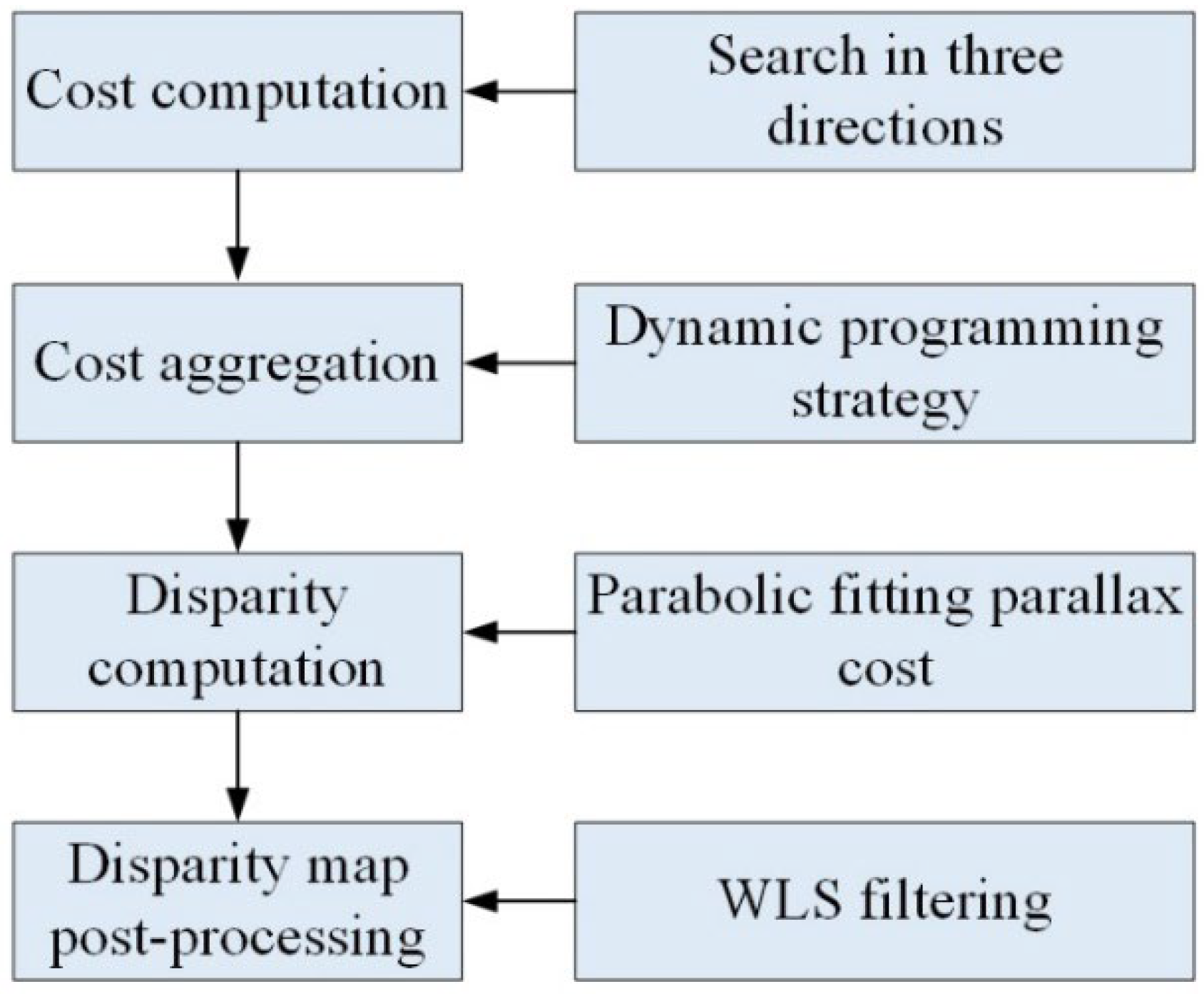
Stereo matching is the most critical and challenging step in binocular vision. An effective stereo-matching algorithm can make key points easier to extract, thereby improving reconstruction accuracy. Semi-global matching (SGM) is a stereo-matching algorithm between local and global matching introduced by Hirschmuller [37]. The core idea of the algorithm is to decompose the global optimization problem into one-dimensional problems, deriving the optimal disparity solution by minimizing the energy function defined in independent directions. This study improves upon the SGM algorithm by proposing a stereo-matching algorithm that calculates costs from multiple directions and can achieve sub-pixel accuracy for disparity values. We named it the MLC-SGM algorithm, which stands for multi-line scanning semi-global matching. Figure 3 illustrates the MLC-SGM algorithm process.

2.5.1. Cost Computation

Cost computation refers to determining the similarity between pixels in the left and right views based on their attributes. The SGM algorithm uses mutual information to evaluate this similarity, which is particularly suitable when there are differences in brightness or contrast between the left and right views. Since this study utilizes images from two different bands, mutual information is also used to compute the pixel-matching cost. The method of calculation is shown in Equation (4).
M I ( X , Y ) = x X , y Y P ( x , y ) log P ( x , y ) P ( x ) P ( y )
where X and Y are the random variables representing the pixel values of the left and right images; P(x) and P(y) are the marginal probability density functions of pixel values x and y in the left and right images, respectively; and P(x, y) is the joint probability density function of pixel values x and y simultaneously appearing at corresponding positions in the left and right images.
In the SGM algorithm, cost computation proceeds from right to left along the epipolar line. This requires high calibration accuracy, as even slight deviations can lead to pixel mismatches. To further enhance the continuity of the pixel search, we added two diagonal directions for cost computation. As shown in Figure 4, when looking for the homonymous points of a pixel in the left image, starting from the same position of the same row in the right image, the maximum disparity search range (maxdis) is set as the radius, and the cost is calculated along the polar line direction and two diagonal lines, respectively. The minimum cost in three directions is taken as the final cost value in each calculation, and the cost in the disparity range of all pixels in the image is stored in the three-dimensional cost space.

2.5.2. Cost Aggregation

Cost aggregation aims to integrate the matching cost of individual pixels into their neighborhoods. This approach enhances disparity continuity, reduces noise impact, and improves matching accuracy and reliability. Hirschmuller [37] introduced multi-path constrained aggregation, which utilizes a dynamic programming strategy to aggregate matching costs from multiple paths. The calculation method is shown in Equations (5) and (6). This study references the aggregation paths of the SGBM algorithm (a variant of the SGM algorithm) and performs cost aggregation along five paths: horizontal, vertical, and left-bottom to right-top.
L r ( p , d ) = C ( p , d ) + min L r ( p r , d ) L r ( p r , d 1 ) + P 1 L r ( p r , d + 1 ) + P 1 min i L r ( p r , i ) + P 2 min i L r ( p r , k )
S ( p , d ) = r L r ( p , d )
where C(p, d) is the initial cost of pixel p at disparity, d; Lr(p, d) is the aggregated cost of pixel p on path r; S(p, d) is the sum of the aggregated costs in all directions; pr represents the position of the preceding pixel on path r; P1 and P2 are disparity change penalties used to penalize minor and significant disparity differences between adjacent pixels, respectively; and miniLr(pr, i) and miniLr(pr, k) are minimization functions used to find the minimum aggregated costs among all possible disparities i and k for the preceding pixel, pr.

2.5.3. Disparity Computation

To enhance the smoothness of the disparity map and improve the accuracy of depth estimation, this study adopts the winner-take-all (WTA) rule for disparity calculation and obtains the disparity value with sub-pixel accuracy by fitting a parabola. As shown in Figure 5, the optimal disparity value corresponding to a homonymous point in the left and right images is assumed to be d, and the matching values at d − 1, d, and d + 1 are C1, C2, and C3, respectively. The disparity value, d*, with sub-pixel accuracy can be obtained by fitting the parabola and solving the parabolic extreme point.

2.5.4. Disparity Map Post-Processing

Disparity map post-processing involves using image processing techniques to smooth and denoise the generated disparity map, enhancing and improving its quality [38]. This study uses weighted least squares (WLSs) filtering for disparity map post-processing because WLS filters assign weights to high-gradient (edge) areas and low-gradient (non-edge) areas separately, applying different levels of smoothing to each. It smooths the image while preserving important edge information as much as possible [39]. The steps for applying WLS filtering to disparity map post-processing are as follows:
  • Compute the horizontal and vertical gradients of each pixel in the disparity map;
  • Set the weights based on the gradient intensity;
  • Adjust pixel values by iteratively solving the weighted least squares loss function for the image.
To better compare the disparity maps of C. hystrix obtained using the SGM algorithm and the proposed MLC-SGM algorithm, the left view after correction was segmented using the threshold method. The resulting binary image was used as a mask on the disparity maps generated by both algorithms, ultimately producing disparity maps containing only the C. hystrix.

2.6. Depth Estimation

The ultimate goal of binocular reconstruction is to establish the correspondence between the spatial physical points and their projections in the left and right views. After obtaining the disparities of corresponding points in the left and right views, the 3D coordinates (Xw, Yw, and Zw) of image pixels in the world coordinate system can be calculated based on the principles of triangulation should be collinearity, as shown in Equations (7)–(9). The height, canopy width, and ground diameter of the C. hystrix can be determined by calculating the Euclidean distance between two points. To evaluate the accuracy of the MLC-SGM algorithm, we calculated the relative error between the algorithm’s measured values and the actual measured values. To ensure the accuracy of manual measurement, a 0.01 cm scale was used to measure the tree height and crown width, and a 0.01 mm vernier caliper was used to measure the ground diameter. Each C. hystrix was measured five times, and after removing the maximum and minimum values, the average of the remaining values was taken as the final measurement result.
X w = b × ( p x c x ) d
Y w = b × ( p y c y ) d
Z w = b × f d
where b is the distance between the optical centers of the left and right cameras, f is the focal length of the left camera after stereo rectification, d is the disparity, px and py are the x and y axis coordinates of the pixel in the left view, and cx and cy are the x and y axis coordinates of the optical center of the left camera.

3. Results

3.1. Comparison of Image Denoising Effect

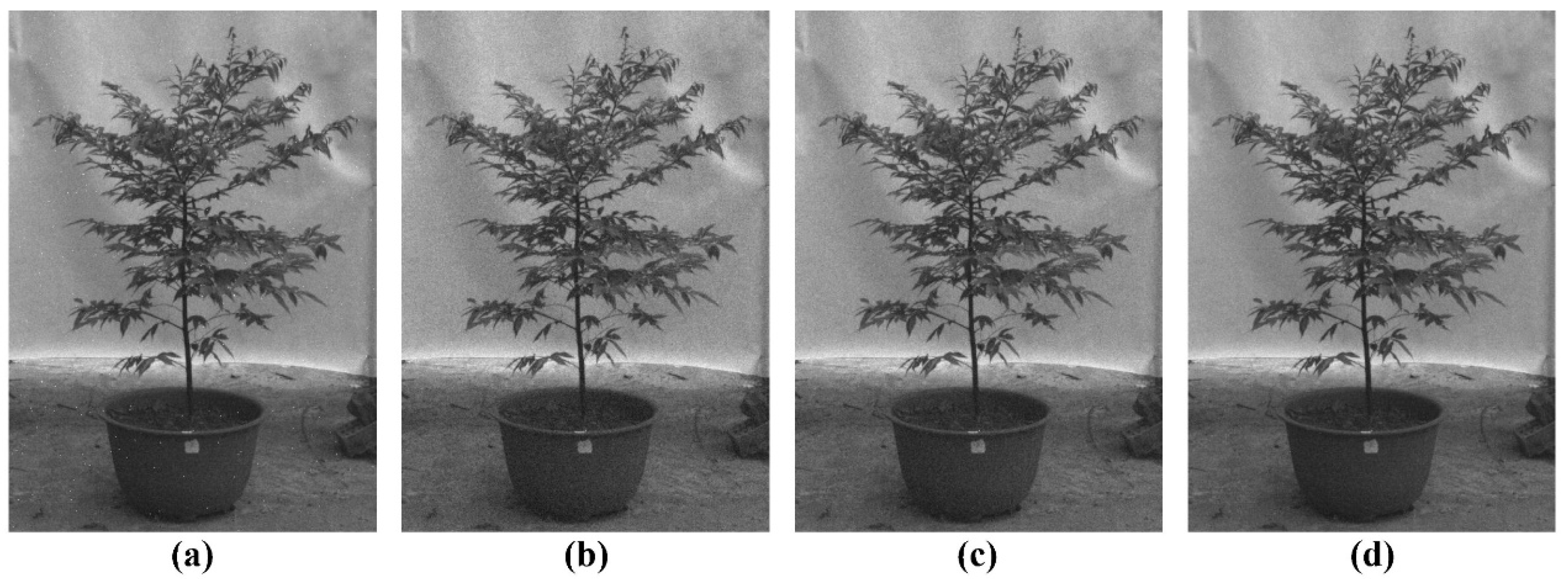
Since noise generation is a random process, to make the analysis results more objective, in addition to the subjective visual effect to determine the denoising effect, we also use the peak signal-to-noise ratio (PSNR) as an objective evaluation index. The higher the PSNR, the less noise remains in the processed image, indicating a better denoising effect. Using a boisterous G-band image as the original image, we applied hard-, soft-, and exponential-decay-thresholding for denoising. Since there is randomly distributed white noise in the image, this study uses the ‘db4’ wavelet that can process high-frequency information components to decompose the image into two layers. It uses the adaptive threshold method to calculate the threshold. The calculated first-layer threshold is 1.37, and the second-layer threshold is 1.02. Figure 6a–d show the noisy image and the denoised results of the three methods, respectively.
Through subjective observation, it can be seen that all three methods remove random noise in the image. However, the image denoised by the wavelet exponential decay threshold method is clearer. To further compare the denoising effects of the three methods and verify the applicability of the ‘db4’ wavelet, the PSNR of the image obtained by using the ‘db4’, ‘db8’, and ‘coif2’ wavelet suitable for processing various signals as the wavelet base is calculated, as shown in Table 1. When the ‘db4’ wavelet is used as the wavelet basis, the exponential decay threshold method improves the PSNR by 5.34% and 2.93% compared with the hard-threshold and soft-threshold methods, respectively. When the ‘db8’ wavelet is used as the wavelet basis, the exponential decay threshold method improves the PSNR by 10.72% and 6.91% compared with the hard-threshold and soft-threshold methods, respectively. When ‘coif2’ is used as the wavelet basis, the image PSNR obtained by the exponential decay threshold method is still higher than that of the hard-threshold and soft-threshold methods, with an increase of 8.60% and 4.76%, respectively. At the same time, the PSNRs when using the ‘db4’ wavelet as the wavelet basis under the three methods are all higher than those of the ‘db8’ and ‘coif2’ wavelets, and the PSNR obtained under the wavelet threshold method is the highest. This shows that the exponential decay threshold denoising method we proposed is superior to the traditional soft-threshold and hard-threshold denoising methods. In practical applications, it can be combined with the appropriate wavelet basis according to the noise characteristics to achieve the best denoising effect.

3.2. Camera Parameters

The 20 pre-captured calibration board images were simultaneously imported using the ‘Load Stereo Images’ feature in the Stereo Camera Calibrator. Then, the ‘Compute Intrinsics’, ‘Radial Distortion’, and ‘Tangential Distortion’ options were selected, and the ‘Calibrate’ function was used for preliminary calibration. Finally, five pairs of images with large reprojection errors were removed to complete the camera calibration. As shown in Table 2, we obtained the principal point coordinates, focal length, radial distortion coefficient, tangential distortion coefficient of the left and right cameras, and rotation and translation matrices of the right camera relative to the left camera. At the same time, to evaluate the accuracy of the camera parameters, we calculated the standard errors of each parameter. The standard error range of the principal point coordinates of the left and right cameras is 1.0~1.3 pixels, and the errors are very close, indicating that the optical center positions of the two cameras are more accurately determined during the calibration process. The standard errors of the focal lengths of the two cameras are also relatively small, ranging from 1.0 to 1.4 pixels. The estimation of the radial distortion and tangential distortion coefficients of the two cameras is more accurate, and the standard errors are less than 0.1. The standard errors of the components of the rotation matrix and the translation matrix are extremely small. The standard errors of the three components of the rotation matrix are 0.0005, 0.0012, and 3.45 × 10⁻⁵ radians, respectively, and the standard errors of the three components of the rotation matrix are 0.0250, 0.0235, and 0.0207 mm, respectively, showing that the estimation results of the rotation angle and translation distance in the three dimensions are very accurate.
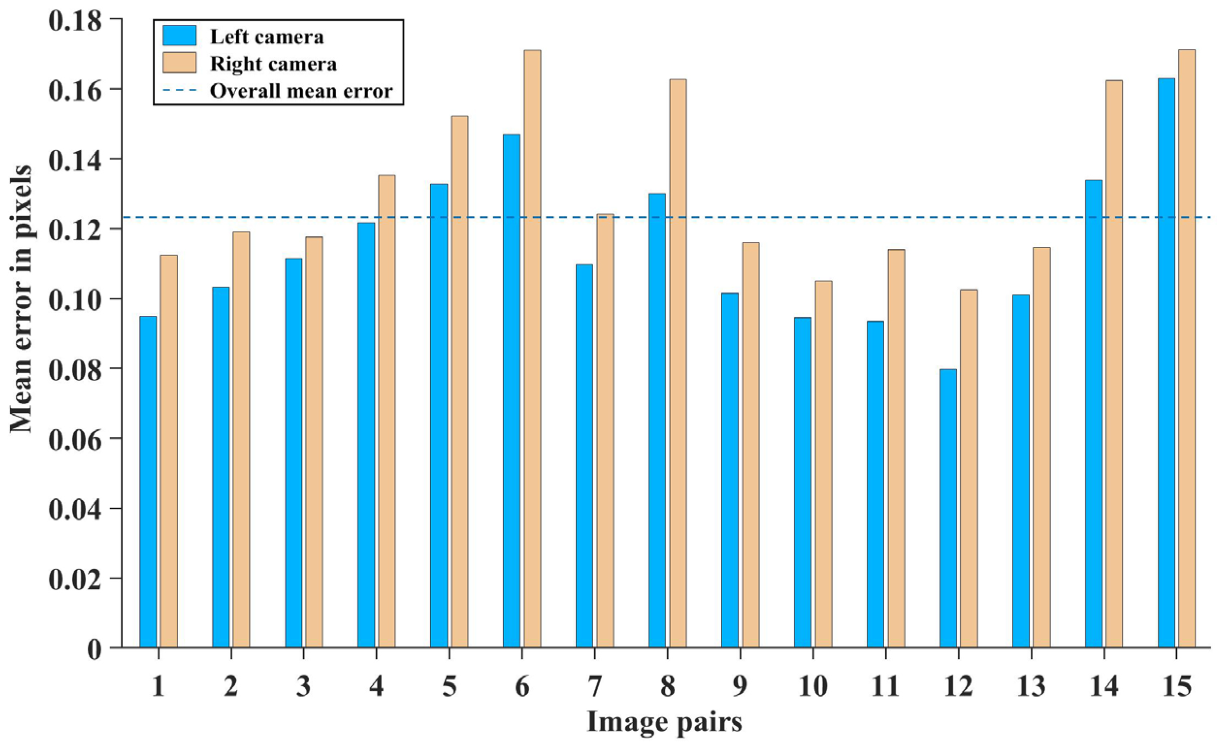
To further verify the effect of camera calibration, we calculated the reprojection errors of 15 pairs of calibration images. In camera calibration, the reprojection error represents the average deviation when a 3D point is reprojected back to the 2D plane. The smaller the value, the more accurate the calibration results. To achieve high-quality reconstruction, the reprojection error should be controlled below 0.5 pixels [40,41]. Figure 7 shows the reprojection error of each checkerboard image. As shown in Figure 7, the reprojection error of the right view (G band) is higher than that of the left view (B band). This is because the noise level of the right view is higher than that of the left view, which is more prone to errors when detecting feature points. However, the difference in the average reprojection error between the left and right views is small, only 0.096 pixels. At the same time, the error of all images is less than 0.18 pixels, and the total average reprojection error is 0.1233 pixels. Combined with the analysis in Table 2, it can be seen that the camera calibration result has a small error and high accuracy.

3.3. Correction Effect

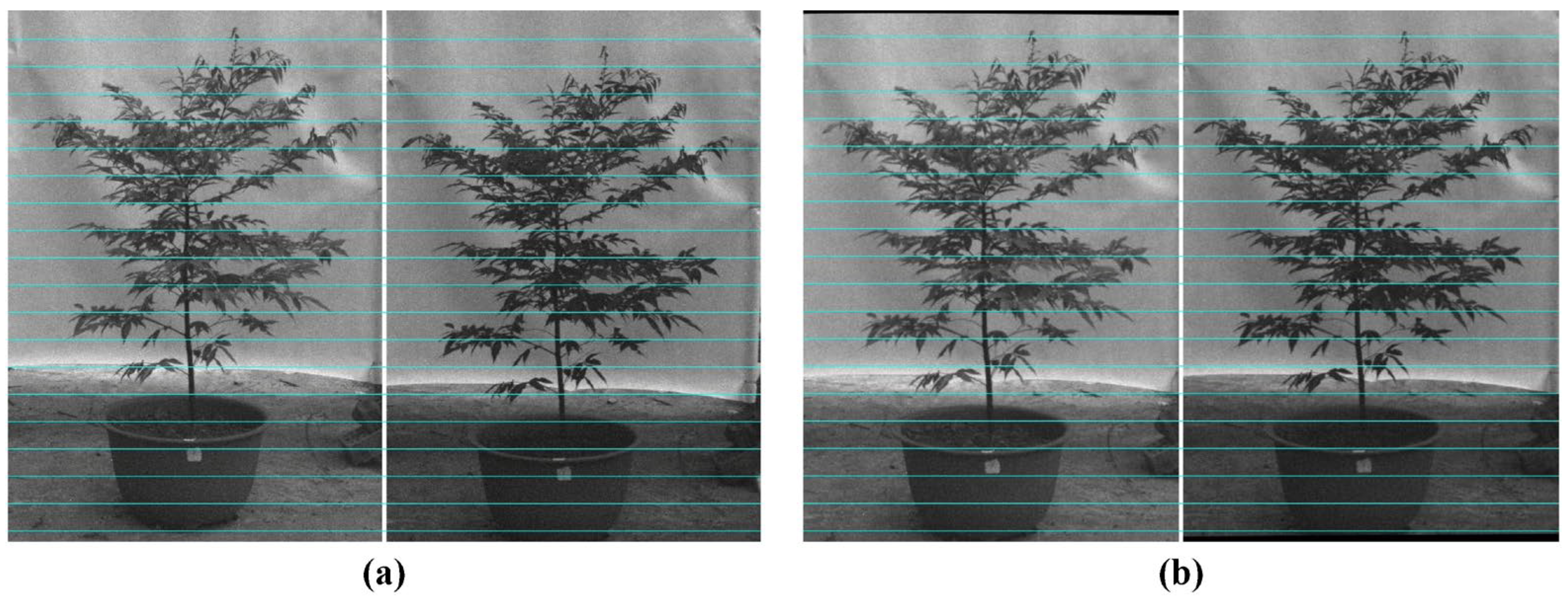
In this study, we first used OpenCV’s stereoRectify function to obtain the stereo rectification parameters, including the rectification rotation matrix and the camera projection matrix for distortion correction. Then, we used the initUndistortRectifyMap function to obtain the mapping matrix. Finally, we applied the mapping matrix to the left and right views using the remap function while interpolating the coordinates, completing the rectification process. To verify the effectiveness of the stereo rectification, horizontal lines were drawn across the image. Figure 8a,b show the left and right image pairs before and after stereo rectification. As shown in Figure 8, stereo rectification eliminated distortion in the left and right images, achieving coplanarity and parallelism and significantly enhancing visual consistency and depth perception.

3.4. Performance of the MLC-SGM Algorithm

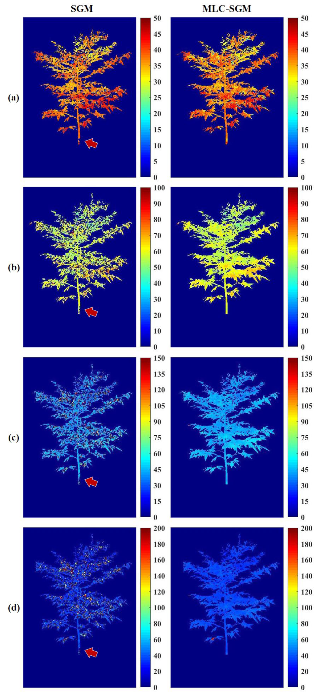
Figure 9a–d are the disparity maps generated by the SGM algorithm and the MLC-SGM algorithm when the maximum disparity value is 50, 100, 150, and 200, respectively. When the maximum disparity value is 50, the disparity maps generated by the SGM algorithm and the MLC-SGM algorithm have no obvious noise, and the PSNR of the disparity maps are 20.56 db and 21.44 db, respectively, showing that the disparity map generated by the MLC-SGM algorithm has less noise and is smoother. When the maximum disparity value is 100, the noise points in the disparity map generated by the SGM algorithm begin to increase, and the PSNR is 19.04 db, while the disparity map generated by the MLC-SGM algorithm has no obvious noise, and the PSNR is 22.59 db, and the image quality is improved. When the maximum disparity value is 150, the noise in the disparity map generated by the SGM algorithm increases significantly, and the PSNR drops to 17.65 db, while the smoothness and continuity of the disparity map generated by the MLC-SGM algorithm remain unchanged, and the PSNR only drops to 21.82 db. When the maximum disparity value is 200, the tree structure of the disparity map generated by the SGM algorithm is clearer, but the noise level also reaches the highest. At this time, the PSNR of the image drops to 14.38 db. Some local noise points also appear in the disparity map generated by the MLC-SGM algorithm, but the PSNR is 20.79 db, which is still above 20 db, indicating that more disparity information is retained. In all settings of the maximum disparity value, the MLC-SGM algorithm shows better disparity continuity and noise suppression than the SGM algorithm. The resulting disparity images are denser and do not exhibit a disparity loss similar to the region indicated by the red arrow. This is because the MLC-SGM algorithm was designed with additional search directions for disparity calculation and included WLS filtering, which helps reduce mismatches and enhance the overall quality of the disparity map.
When the maximum disparity value is set to 50, the disparity maps generated by the MLC-SGM and SGM algorithms both have a certain degree of edge missing. This is because the search range is too small, resulting in the inability to correctly match the edge points with the same name in the left and right views. When the maximum disparity value is set to 150 and 200, the left edge of the disparity images generated by the MLC-SGM and SGM algorithms gradually disappears. This happens because the set maximum disparity exceeds the actual disparity range of the image pair, leading to specific areas in the left image lacking corresponding matching parts in the right image. However, compared to the SGM algorithm, the MLC-SGM algorithm handles this issue better because the WLS filter smooths the disparity map while preserving the image edge, enhancing the disparity map’s continuity. The above analysis indicates that the MLC-SGM algorithm performs better than the SGM algorithm when dealing with complex structures and textures in scenes like trees. Under the conditions of this study, the matching effect is best when the maximum disparity value is set to 100.
Table 3 shows the relative errors of tree height, canopy width, and ground diameter measurements for 64 C. hystrix trees obtained using the SGM and MLC-SGM algorithms compared to the actual values. The SGM algorithm’s relative error range for tree height was from 2.51% to 4.84%; for canopy width, it was from 3.65% to 6.98%; and for ground diameter, it was from 2.89% to 5.79%. The MLC-SGM algorithm’s relative error range for tree height was from 1.85% to 3.91%; for canopy width, it was from 1.89% to 4.64%; and for ground diameter, it was from 2.21% to 4.53%. Compared to the SGM algorithm, the MLC-SGM algorithm produced smaller error ranges for tree height, canopy width, and ground diameter. In terms of average error, the MLC-SGM algorithm reduced errors in tree height, canopy width, and ground diameter by 29.22%, 27.93%, and 32.49%, respectively, compared to the SGM algorithm. Across all measurement indicators, the MLC-SGM algorithm demonstrated better accuracy and stability than the SGM algorithm. This indicates that the MLC-SGM algorithm is more efficient in handling texture and occlusion in C. hystrix images. Overall, the MLC-SGM algorithm offers greater measurement accuracy compared to the SGM algorithm.

3.5. Growth Differences of C. hystrix at Different Nitrogen Levels

As shown in Figure 10a, compared to the CK group, the height growth of the T2 and T3 groups significantly increased by 17.25% and 19.07% (p < 0.001), respectively. Compared to the T1 group, the height growth of the T2 and T3 groups significantly increased by 12.56% and 14.31% (p < 0.01), respectively. However, there were no significant differences in height growth between the CK and T1 groups or between the T2 and T3 groups. This shows that, compared with no fertilization and low nitrogen fertilization, medium nitrogen fertilization and high nitrogen fertilization can significantly promote the height growth of C. hystrix, and there is no significant difference in the promotion effect.
As shown in Figure 10b, compared to the CK group, the canopy width growth of the T2 group significantly increased by 18.82% (p < 0.001), while the T3 group increased by 14.83% (p < 0.01). Compared to the T1 group, the T2 group significantly increased by 9.16% (p < 0.05). However, there were no significant differences in canopy width growth between the CK and T1 groups, the T1 and T3 groups, or the T2 and T3 groups. This shows that, compared with no fertilization and low nitrogen fertilization, both medium and high nitrogen fertilization can promote the growth of crown width of C. hystrix, but the promoting effect of high nitrogen fertilization on crown width growth is weaker than that of medium nitrogen fertilization.
As shown in Figure 10c, compared to the CK group, the ground diameter growth of the T1, T2, and T3 groups significantly increased by 23.58%, 34.21%, and 24.45% (p < 0.001), respectively. However, there were no significant differences among the T1, T2, and T3 groups. This shows that, compared to no fertilization, low, medium, and high nitrogen fertilization can all promote the ground diameter growth of C. hystrix. However, over-fertilization can slow down the ground diameter’s growth rate.

4. Discussion

4.1. Precise Matching of Plant Images

Subtle differences between image pairs will significantly reduce the accuracy of stereo matching. Plants are non-rigid objects, and their environment constantly changes, thus further increasing the complexity of matching [25,42]. An accurate stereo-matching algorithm can ensure a high-quality disparity map, making the depth-estimation results more precise. This is of great significance for measurement work in agriculture and forestry. Lati et al. [43] used the DP algorithm for stereo matching in their binocular vision system, achieving reconstruction of sunflower and corn plants, with measurement errors in plant height ranging from 4.1% to 5.1% and from 3.9% to 5.6%, respectively. Malekabadi et al. [4] used the AGBM algorithm for disparity computation to analyze tree geometry, achieving measurement errors ranging from −8% to 5% for tree height and from −1% to 3% for trunk width. Yuan et al. [26] applied the BM algorithm for matching seedling image pairs, with an average measurement error of 4.94% for the height of 247 seedlings.
Our approach is more accurate than these methods, with average measurement errors of less than 3.1% for tree height, canopy width, and ground diameter. This is because the MLC-SGM algorithm we proposed adds the direction of cost search, which effectively reduces the mismatch rate and improves the quality of the disparity map. Although the MLC-SGM algorithm increased computational load somewhat, its accuracy gain is desirable for many applications, especially in agriculture and forestry, where measurement accuracy is critical. In theory, more search directions result in more accurate cost computation but consume more computational resources. Considering the matching efficiency, this study only added two search directions, so the improvement in measurement accuracy is relatively small. At the same time, this study did not consider the impact of camera angle transformation on measurement accuracy. In future studies, images will be acquired from multiple angles, and the balance between algorithm calculation efficiency and matching accuracy will be explored in depth to provide a better solution for high-precision stereo matching of real trees.

4.2. Optimization of Tree Fertilization Strategy

Compared to traditional manual measurements, using binocular vision methods to reconstruct tree growth factors can minimize disturbance to natural growth conditions and allow for the measurement of many samples quickly, providing data with greater repeatability and comparability. These data are precious in statistical analysis because they can more accurately reveal differences in tree growth factors under different fertilization levels and determine which fertilization method is most conducive to tree growth, thereby guiding the development of fertilization plans more precisely [44]. Reconstructing tree growth factors through binocular vision technology provides a non-invasive, efficient, and reliable measurement method for forestry production and helps determine the optimal fertilization amount. This enhances forestry production’s efficiency and sustainability while reducing resource overuse and negative environmental impacts.
In this study, we used binocular reconstruction technology to measure the differences in height, canopy width, and ground diameter growth of C. hystrix under different nitrogen application levels and analyzed the specific effects of nitrogen application on C. hystrix growth. This provides a reference for nitrogen fertilization of valuable tree species like C. hystrix. Besides nitrogen, phosphorus, potassium, magnesium, and iron play key roles in tree nutrition and health. Properly supplying these elements is crucial for ensuring tree growth, physiological functions, and yield [45,46]. In future research, we will further investigate the effects of different elements on the growth of C. hystrix based on the current findings and explore the interactions and synergistic effects between these elements, providing more scientific and precise fertilization guidance for the production and cultivation of C. hystrix.

5. Conclusions

This study used two single-band cameras from the MicaSense RedEdge multispectral imager to form a binocular vision system for measuring the height, canopy width, and ground diameter growth of C. hystrix while also analyzing the effects of different fertilization levels on its development. In this research, we designed a new threshold function (exponential decay threshold function) to denoise the images of the C. hystrix. We also improved the SGM algorithm and proposed the MLC-SGM stereo-matching algorithm. By analyzing the disparity images and the measurement errors of the algorithm, we evaluated the performance of the MLC-SGM algorithm. The results indicate the following:
  • The exponential decay threshold function effectively removes random noise from the images of Castanopsis hystrix, and its denoising effect is superior to hard- and soft-threshold functions.
  • The MLC-SGM algorithm produces higher-quality disparity maps than the SGM algorithm and results in lower measurement errors for the growth factors of C. hystrix. The average relative errors in height, canopy width, and ground diameter for 64 trees were 2.35%, 3.07%, and 2.93%, respectively.
  • Medium nitrogen fertilization significantly promotes the height, canopy width, and ground diameter growth of C. hystrix, but this promoting effect diminishes when over-fertilization occurs, with more significant impacts on canopy width and ground diameter growth.

Author Contributions

P.W. performed the experiments, analyzed the data, and wrote the manuscript; X.W. designed the research and conducted the field measurements and collected the samples; X.C. and M.S. analyzed the data. All authors have read and agreed to the published version of the manuscript.

Funding

This research was funded by the National Natural Science Foundation of China’s “Machine Understanding Method of Forest Nutrient and Moisture Requirement”, grant number 32071761.

Data Availability Statement

The data presented in this study are available upon request from the corresponding author. The data are not publicly available due to the confidentiality of the project.

Acknowledgments

We acknowledge the support from the IFRIT of CAF.

Conflicts of Interest

The authors declare no conflict of interest.

References

  1. Fan, G.; Feng, W.; Chen, F.; Chen, D.; Dong, Y.; Wang, Z. Measurement of volume and accuracy analysis of standing trees using Forest Survey Intelligent Dendrometer. Comput. Electron. Agric. 2020, 169, 105211. [Google Scholar] [CrossRef]
  2. Jurjević, L.; Liang, X.; Gašparović, M.; Balenović, I. Is field-measured tree height as reliable as believed–Part II, A comparison study of tree height estimates from conventional field measurement and low-cost close-range remote sensing in a deciduous forest. ISPRS-J. Photogramm. Remote Sens. 2020, 169, 227–241. [Google Scholar] [CrossRef]
  3. Méndez, V.; Rosell-Polo, J.R.; Pascual, M.; Escola, A. Multi-tree woody structure reconstruction from mobile terrestrial laser scanner point clouds based on a dual neighbourhood connectivity graph algorithm. Biosyst. Eng. 2016, 148, 34–47. [Google Scholar] [CrossRef]
  4. Malekabadi, A.J.; Khojastehpour, M.; Emadi, B. Disparity map computation of tree using stereo vision system and effects of canopy shapes and foliage density. Comput. Electron. Agric. 2019, 156, 627–644. [Google Scholar] [CrossRef]
  5. Wilkes, P.; Lau, A.; Disney, M.; Calders, K.; Burt, A.; de Tanago, J.G.; Herold, M. Data acquisition considerations for terrestrial laser scanning of forest plots. Remote Sens. Environ. 2017, 196, 140–153. [Google Scholar] [CrossRef]
  6. Burgess, A.J.; Retkute, R.; Herman, T.; Murchie, E.H. Exploring relationships between canopy architecture, light distribution, and photosynthesis in contrasting rice genotypes using 3D canopy reconstruction. Front. Plant Sci. 2017, 8, 734. [Google Scholar] [CrossRef]
  7. Cuevas-Velasquez, H.; Gallego, A.J.; Fisher, R.B. Segmentation and 3D reconstruction of rose plants from stereoscopic images. Comput. Electron. Agric. 2020, 171, 105296. [Google Scholar] [CrossRef]
  8. Yang, T.; Ye, J.; Zhou, S.; Xu, A.; Yin, J. 3D reconstruction method for tree seedlings based on point cloud self-registration. Comput. Electron. Agric. 2022, 200, 107210. [Google Scholar] [CrossRef]
  9. Xiang, L.; Gai, J.; Bao, Y.; Yu, J.; Schnable, P.S.; Tang, L. Field-based robotic leaf angle detection and characterization of maize plants using stereo vision and deep convolutional neural networks. J. Field Robot. 2023, 40, 1034–1053. [Google Scholar] [CrossRef]
  10. Dassot, M.; Constant, T.; Fournier, M. The use of terrestrial LiDAR technology in forest science: Application fields, benefits and challenges. Ann. For. Sci. 2011, 68, 959–974. [Google Scholar] [CrossRef]
  11. Chau, W.Y.; Loong, C.N.; Wang, Y.H.; Chiu, S.W.; Tan, T.J.; Wu, J.; Mei, L.L.; Tan, P.S.; Ooi, G.L. Understanding the dynamic properties of trees using the motions constructed from multi-beam flash light detection and ranging measurements. J. R. Soc. Interface 2022, 19, 20220319. [Google Scholar] [CrossRef]
  12. Raumonen, P.; Kaasalainen, M.; Åkerblom, M.; Kaasalainen, S.; Kaartinen, H.; Vastaranta, M.; Lewis, P. Fast automatic precision tree models from terrestrial laser scanner data. Remote Sens. 2013, 5, 491–520. [Google Scholar] [CrossRef]
  13. Lau, A.; Bentley, L.P.; Martius, C.; Shenkin, A.; Bartholomeus, H.; Raumonen, P.; Malhi, Y.; Jackson, T.; Herold, M. Quantifying branch architecture of tropical trees using terrestrial LiDAR and 3D modelling. Trees 2018, 32, 1219–1231. [Google Scholar] [CrossRef]
  14. Gamarra-Diezma, J.L.; Miranda-Fuentes, A.; Llorens, J.; Cuenca, A.; Blanco-Roldán, G.L.; Rodríguez-Lizana, A. Testing accuracy of long-range ultrasonic sensors for olive tree canopy measurements. Sensors 2015, 15, 2902–2919. [Google Scholar] [CrossRef] [PubMed]
  15. Yu, Z.; Zhang, B. A camera/ultrasonic sensors based trunk localization system of semi-structured orchards. In Proceedings of the 2021 IEEE/ASME International Conference on Advanced Intelligent Mechatronics (AIM), Delft, The Netherlands, 12–16 July 2021. [Google Scholar]
  16. Colaço, A.F.; Molin, J.P.; Rosell-Polo, J.R.; Escolà, A. Application of light detection and ranging and ultrasonic sensors to high-throughput phenotyping and precision horticulture: Current status and challenges. Hortic. Res. 2018, 5, 35. [Google Scholar] [CrossRef]
  17. Bongers, F. Methods to assess tropical rain forest canopy structure: An overview. In Tropical Forest Canopies: Ecology and Management, Proceedings of the ESF Conference, Oxford University, Oxford, UK, 12–16 December 1998; Springer: Berlin/Heidelberg, Germany, 1998. [Google Scholar]
  18. Duan, T.; Chapman, S.C.; Holland, E.; Rebetzke, G.; Guo, Y.; Zheng, B. Dynamic quantification of canopy structure to characterize early plant vigour in wheat genotypes. J. Exp. Bot. 2016, 67, 4523–4534. [Google Scholar] [CrossRef]
  19. Golbach, F.; Kootstra, G.; Damjanovic, S.; Otten, G.; van de Zedde, R. Validation of plant part measurements using a 3D reconstruction method suitable for high-throughput seedling phenotyping. Mach. Vis. Appl. 2016, 27, 663–680. [Google Scholar] [CrossRef]
  20. Li, Y.; Zhang, Z.; Wang, X.; Fu, W.; Li, J. Automatic reconstruction and modeling of dormant jujube trees using three-view image constraints for intelligent pruning applications. Comput. Electron. Agric. 2023, 212, 108149. [Google Scholar] [CrossRef]
  21. Lu, X.; Ono, E.; Lu, S.; Zhang, Y.; Teng, P.; Aono, M.; Omasa, K. Reconstruction method and optimum range of camera-shooting angle for 3D plant modeling using a multi-camera photography system. Plant Methods 2020, 16, 118. [Google Scholar] [CrossRef]
  22. Liu, L.; Liu, Y.; Lv, Y.; Li, X. A Novel Approach for Simultaneous Localization and Dense Mapping Based on Binocular Vision in Forest Ecological Environment. Forests 2024, 15, 147. [Google Scholar] [CrossRef]
  23. Yi, H.; Song, K.; Song, X. Watermelon Detection and Localization Technology based on GTR-Net and Binocular Vision. IEEE Sens. J. 2024, 24, 19873–19881. [Google Scholar] [CrossRef]
  24. Li, D.; Xu, L.; Tang, X.; Sun, S.; Cai, X.; Zhang, P. 3D imaging of greenhouse plants with an inexpensive binocular stereo vision system. Remote Sens. 2017, 9, 508. [Google Scholar] [CrossRef]
  25. Peng, Y.; Yang, M.; Zhao, G.; Cao, G. Binocular-vision-based structure from motion for 3-D reconstruction of plants. IEEE Geosci. Remote Sens. Lett. 2021, 19, 8019505. [Google Scholar] [CrossRef]
  26. Yuan, X.; Li, D.; Sun, P.; Wang, G.; Ma, Y. Real-Time Counting and Height Measurement of Nursery Seedlings Based on Ghostnet–YoloV4 Network and Binocular Vision Technology. Forests 2022, 13, 1459. [Google Scholar] [CrossRef]
  27. Fu, K.; Yue, S.; Yin, B. DBH Extraction of Standing Trees Based on a Binocular Vision Method. In Proceedings of the 2023 IEEE International Instrumentation and Measurement Technology Conference (I2MTC), Kuala Lumpur, Malaysia, 22–25 May 2023. [Google Scholar]
  28. Ni, Z.; Burks, T.F.; Lee, W.S. 3D reconstruction of plant/tree canopy using monocular and binocular vision. J. Imaging 2016, 2, 28. [Google Scholar] [CrossRef]
  29. Zhang, R.; Lian, S.; Li, L.; Zhang, L.; Zhang, C.; Chen, L. Design and experiment of a binocular vision-based canopy volume extraction system for precision pesticide application by UAVs. Comput. Electron. Agric. 2023, 213, 108197. [Google Scholar] [CrossRef]
  30. Saarsalmi, A.; Mälkönen, E. Forest fertilization research in Finland: A literature review. Scand. J. For. Res. 2001, 16, 514–535. [Google Scholar] [CrossRef]
  31. Gaige, E.; Dail, D.B.; Hollinger, D.Y.; Davidson, E.A.; Fernandez, I.J.; Sievering, H.; Halteman, W. Changes in canopy processes following whole-forest canopy nitrogen fertilization of a mature spruce-hemlock forest. Ecosystems 2007, 10, 1133–1147. [Google Scholar] [CrossRef]
  32. Zheng, B.; Xiang, Z.; Qaseem, M.F.; Zhao, S.; Li, H.; Feng, J.X.; Stolarski, M.J. Characterization of hemicellulose during xylogenesis in rare tree species Castanopsis hystrix. Int. J. Biol. Macromol. 2022, 212, 348–357. [Google Scholar]
  33. Rizkinia, M.; Baba, T.; Shirai, K.; Okuda, M. Local spectral component decomposition for multi-channel image denoising. IEEE Trans. Image Process. 2016, 25, 3208–3218. [Google Scholar] [CrossRef]
  34. Tian, C.; Zheng, M.; Zuo, W.; Zhang, B.; Zhang, Y.; Zhang, D. Multi-stage image denoising with the wavelet transform. Pattern Recognit. 2023, 134, 109050. [Google Scholar] [CrossRef]
  35. Zhang, Z. Flexible camera calibration by viewing a plane from unknown orientations. In Proceedings of the Seventh IEEE International Conference on Computer Vision, Kerkyra, Greece, 20–27 September 1999. [Google Scholar]
  36. Zhang, Z. Determining the epipolar geometry and its uncertainty: A review. Int. J. Comput. Vis. 1998, 27, 161–195. [Google Scholar] [CrossRef]
  37. Hirschmuller, H. Stereo processing by semiglobal matching and mutual information. IEEE Trans. Pattern Anal. Mach. Intell. 2007, 30, 328–341. [Google Scholar] [CrossRef]
  38. Ma, Y.; Fang, X.; Guan, X.; Li, K.; Chen, L.; An, F. Five-Direction Occlusion Filling with Five Layer Parallel Two-Stage Pipeline for Stereo Matching with Sub-Pixel Disparity Map Estimation. Sensors 2022, 22, 8605. [Google Scholar] [CrossRef] [PubMed]
  39. Huang, Z.; Zhu, Z.; An, Q.; Wang, Z.; Fang, H. Global–local image enhancement with contrast improvement based on weighted least squares. Optik 2021, 243, 167433. [Google Scholar] [CrossRef]
  40. Bradley, D.; Heidrich, W. Binocular camera calibration using rectification error. In Proceedings of the 2010 Canadian Conference on Computer and Robot Vision, Ottawa, ON, Canada, 31 May–2 June 2010. [Google Scholar]
  41. Tabb, A.; Yousef, K.M.A. Parameterizations for reducing camera reprojection error for robot-world hand-eye calibration. In Proceedings of the 2015 IEEE/RSJ International Conference on Intelligent Robots and Systems (IROS), Hamburg, Germany, 28 September–2 October 2015. [Google Scholar]
  42. Zhang, Y.; Gu, J.; Rao, T.; Lai, H.; Zhang, B.; Zhang, J.; Yin, Y. A shape reconstruction and measurement method for spherical hedges using binocular vision. Front. Plant Sci. 2022, 13, 849821. [Google Scholar] [CrossRef]
  43. Lati, R.N.; Filin, S.; Eizenberg, H. Estimating plant growth parameters using an energy minimization-based stereovision model. Comput. Electron. Agric. 2013, 98, 260–271. [Google Scholar] [CrossRef]
  44. Guo, J.; Wu, Y.; Wang, B.; Lu, Y.; Cao, F.; Wang, G. The effects of fertilization on the growth and physiological characteristics of Ginkgo biloba L. Forests 2016, 7, 293. [Google Scholar] [CrossRef]
  45. Santiago, L.S.; Wright, S.J.; Harms, K.E.; Yavitt, J.B.; Korine, C.; Garcia, M.N.; Turner, B.L. Tropical tree seedling growth responses to nitrogen, phosphorus and potassium addition. J. Ecol. 2012, 100, 309–316. [Google Scholar] [CrossRef]
  46. Kwakye, S.; Kadyampakeni, D.M.; Morgan, K.; Vashisth, T.; Wright, A. Effects of iron rates on growth and development of young huanglongbing-affected citrus trees in Florida. HortScience 2022, 57, 1092–1098. [Google Scholar] [CrossRef]
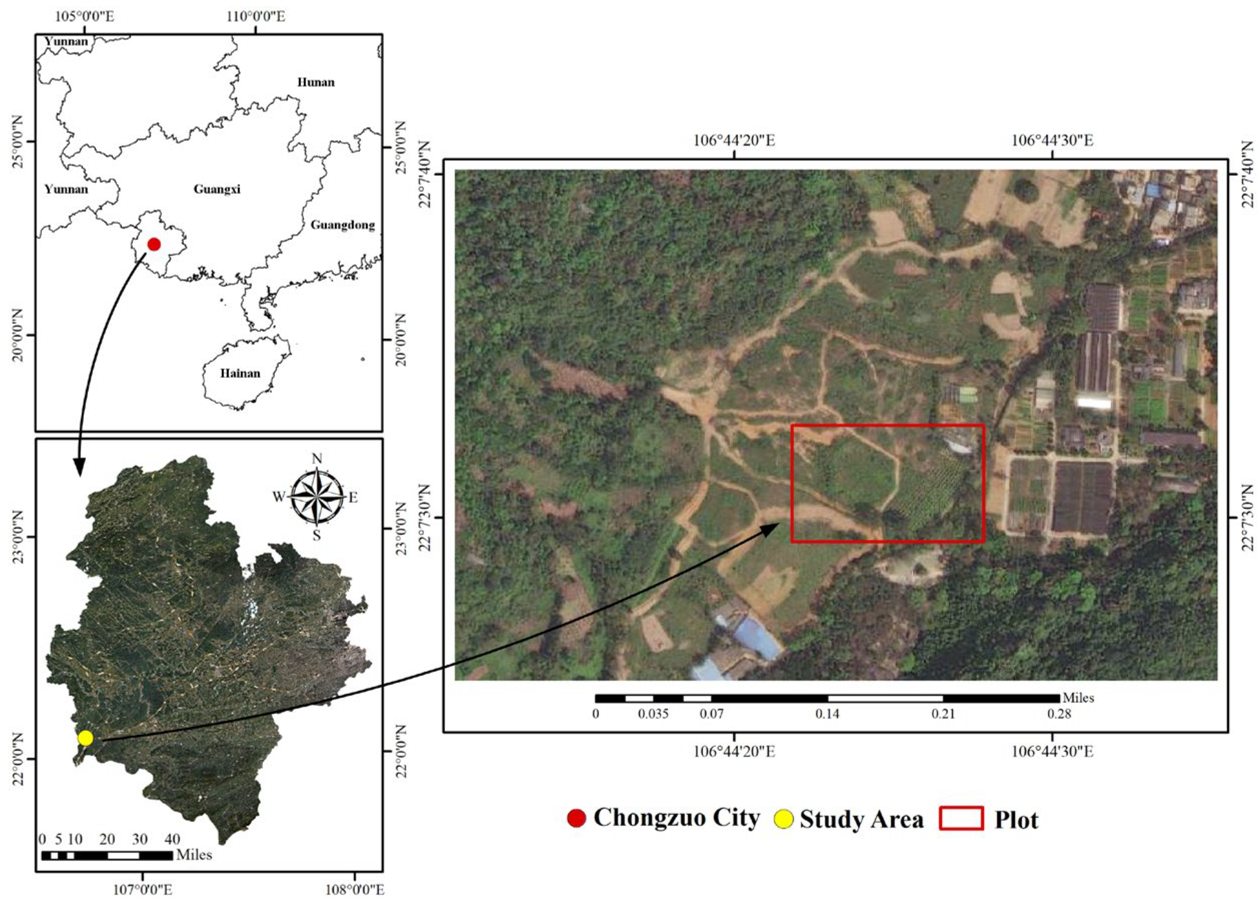
Figure 1. Study-area location map.
Forests 15 01558 g001
Figure 2. Schematic diagram of epipolar geometry.
Forests 15 01558 g002
Figure 3. MLC-SGM algorithm process.
Forests 15 01558 g003
Figure 4. Schematic diagram of cost calculation: (a) left image and (b) right image.
Forests 15 01558 g004
Figure 5. Parabolic fit with sub-pixel accuracy parallax.
Forests 15 01558 g005
Figure 6. Image-denoising results: (a) noisy image, (b) hard-thresholding denoised image, (c) soft-thresholding denoised image, and (d) exponential decay-thresholding denoised image.
Forests 15 01558 g006
Figure 7. Image reprojection error.
Forests 15 01558 g007
Figure 8. Comparison before and after image correction: (a) uncorrected binocular images and (b) corrected binocular images.
Forests 15 01558 g008
Figure 9. Parallax image realized by SGM and MLC-SGM algorithm: (a) maximum parallax = 50; (b) maximum parallax = 100; (c) maximum parallax = 150; and (d) maximum parallax = 200.
Forests 15 01558 g009
Figure 10. Difference significance of C. hystrix growth in four groups: (a) tree height, (b) crowth, and (c) ground diameter. * stands for 95% confidence level, ** stands for 99% confidence level, and *** stands for 99.9% confidence level.
Forests 15 01558 g010
Table 1. PSNR of 3 denoising methods.
MethodPSNR (db)
db4db8coif2
Hard threshold29.0126.9625.93
Soft threshold29.6927.9226.88
Exponential decay threshold30.5629.8528.16
Table 2. Camera calibration parameters and standard errors.
Camera
Parameters
Left CameraStandard ErrorRight CameraStandard Error
Principal point
coordinates
1440.6182 1442.9894 1.1484 1.2330 1444.6925 1447.3360 1.0475 1.2175
Focal length 645.8878 454.8982 1.0706 1.3619 645.5077 147.3360 1.1269 1.2934
Radial distortion
coefficient
0.0621 0.0868 0.6276 0.0105 0.0082 0.0981 0.0702 0.0633 0.0758 0.0102 0.0167 0.0411
Tangential distortion
coefficient
0.0031 0.0003 0.0002 0.0001 0.0031 0.0003 0.0001 0.0001
Rotation matrix 1 0.0019 0.0005 0.0019 1 0.0097 0.0005 0.0097 1 0.0005 0.0012 3.45 × 10 5
Translation matrix 30.0460 0.0156 0.5539 0.0250 0.0235 0.0207
Table 3. Comparison of measurement accuracy between SGM and MLC-SGM algorithms.
Growth FactorSGMMLC-SGM
Relative Error
(%)
Average Error (%)Relative Error (%)Average Error (%)
Tree height2.51~4.843.321.85~3.912.35
Canopy width3.65~6.984.261.89~4.643.07
Ground diameter2.89~5.794.342.21~4.532.93
Disclaimer/Publisher’s Note: The statements, opinions and data contained in all publications are solely those of the individual author(s) and contributor(s) and not of MDPI and/or the editor(s). MDPI and/or the editor(s) disclaim responsibility for any injury to people or property resulting from any ideas, methods, instructions or products referred to in the content.