
Modeling the Spatial Distribution of Acacia decurrens Plantation Forests Using PlanetScope Images and Environmental Variables in the Northwestern Highlands of Ethiopia

Abstract
:1. Introduction
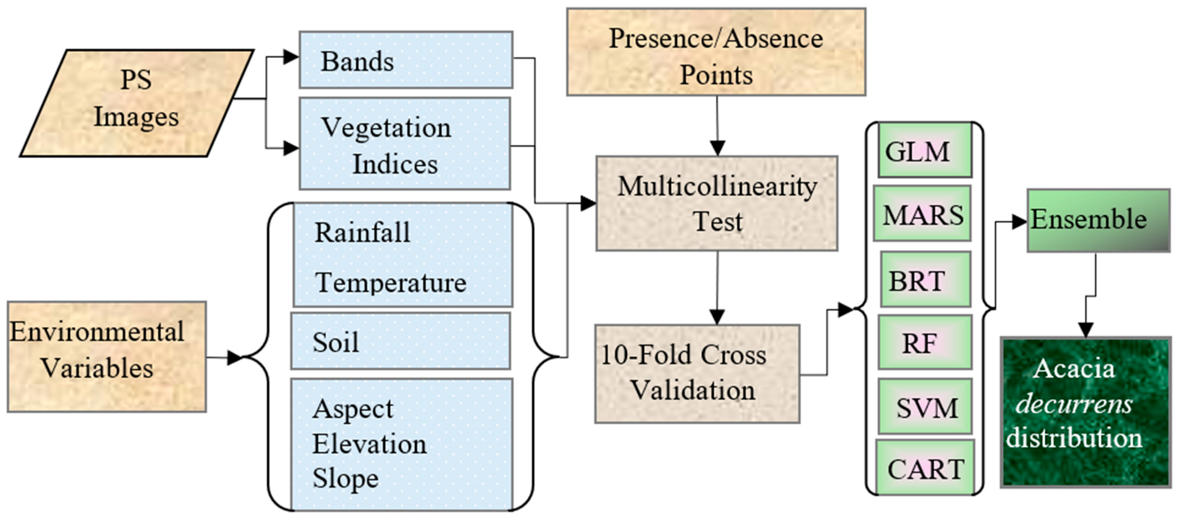
2. Data and Methods
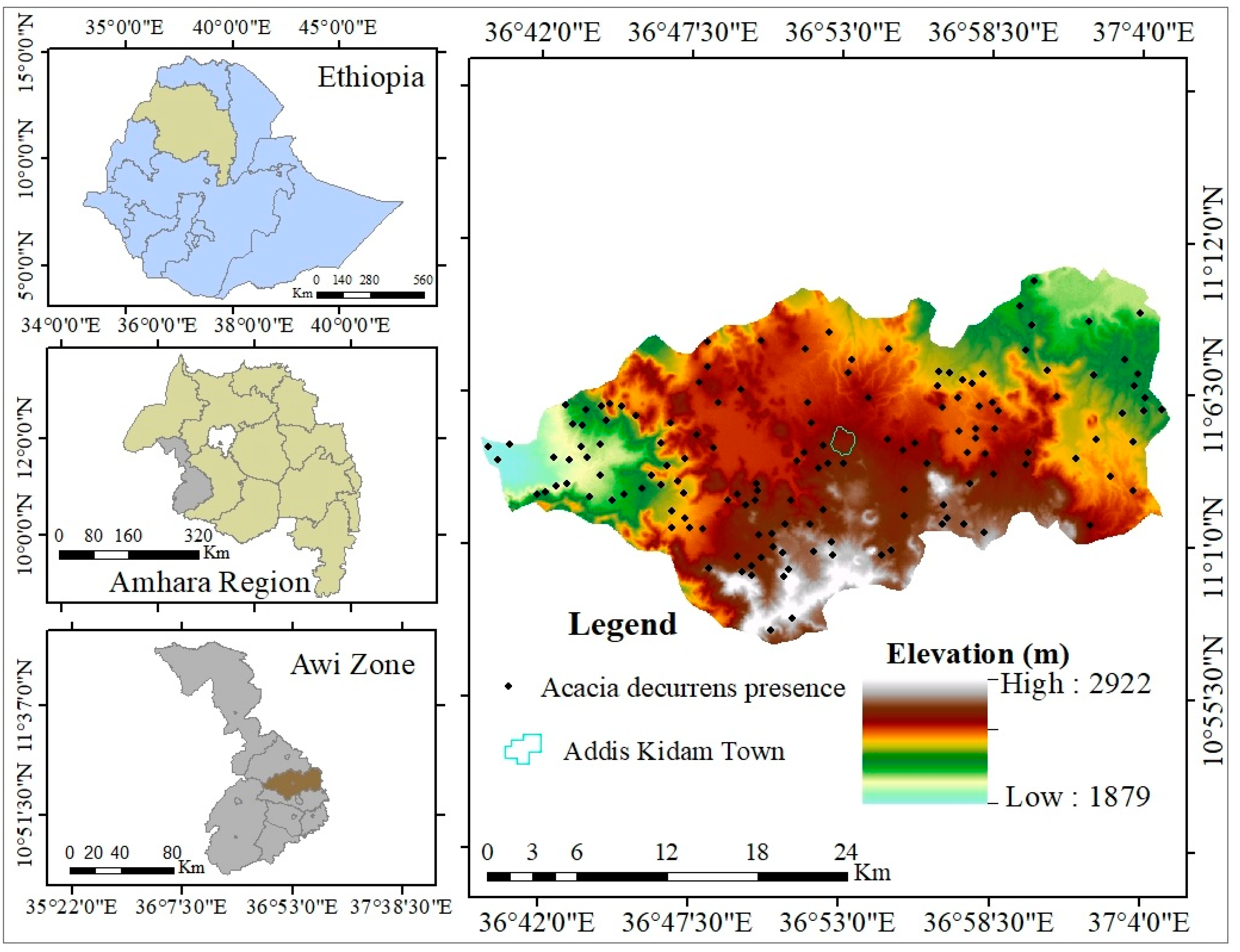
2.1. Study Area
2.2. Data
2.2.1. Remote Sensing Data
2.2.2. Environmental Variable Data
2.2.3. Presence/Absence Data
2.3. Variable Selection
2.4. Modelling Algorithms
2.5. Model Evaluation
3. Results
3.1. Multicollinearity Test
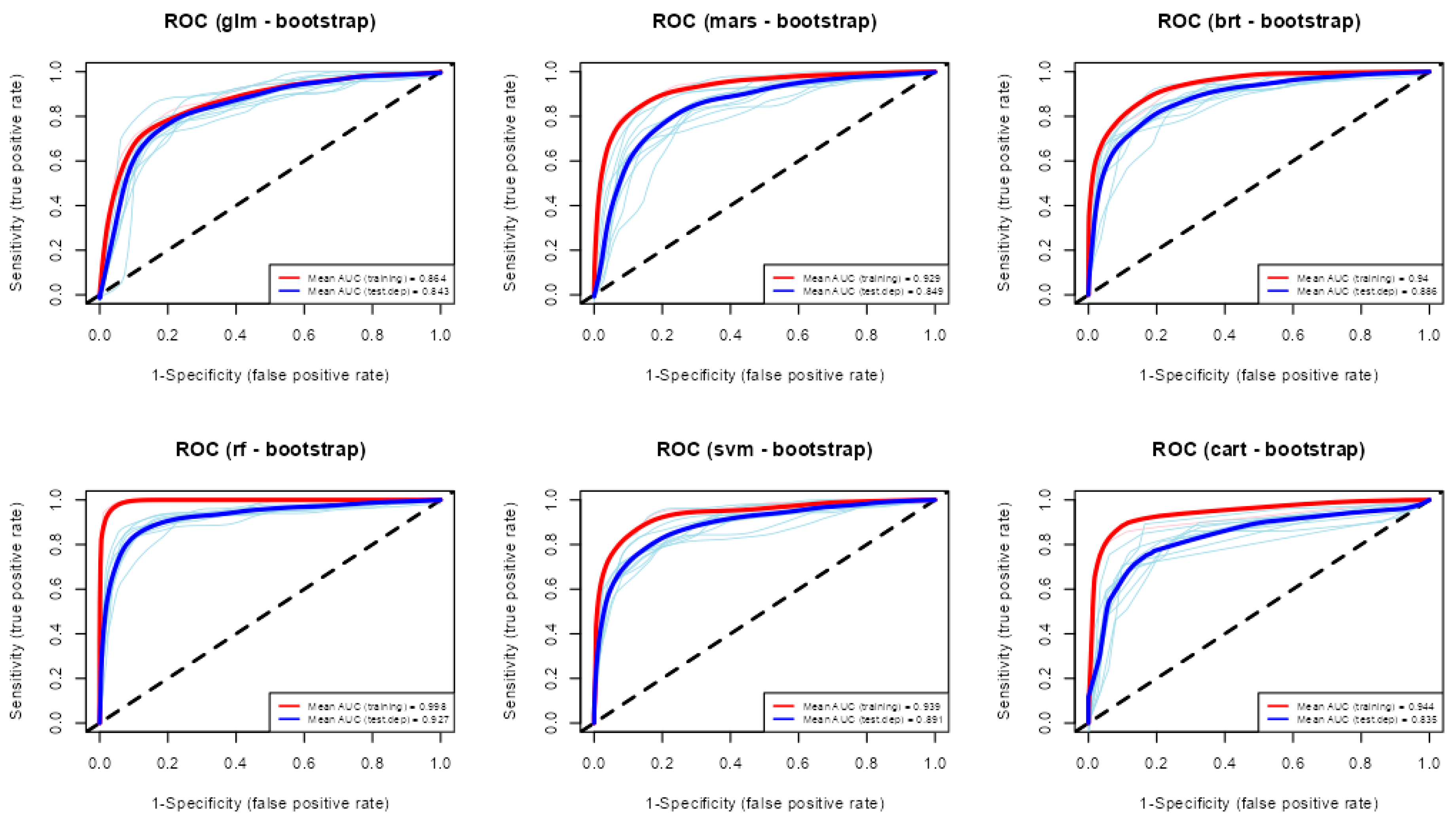
3.2. Performance of Modelling Algorithms
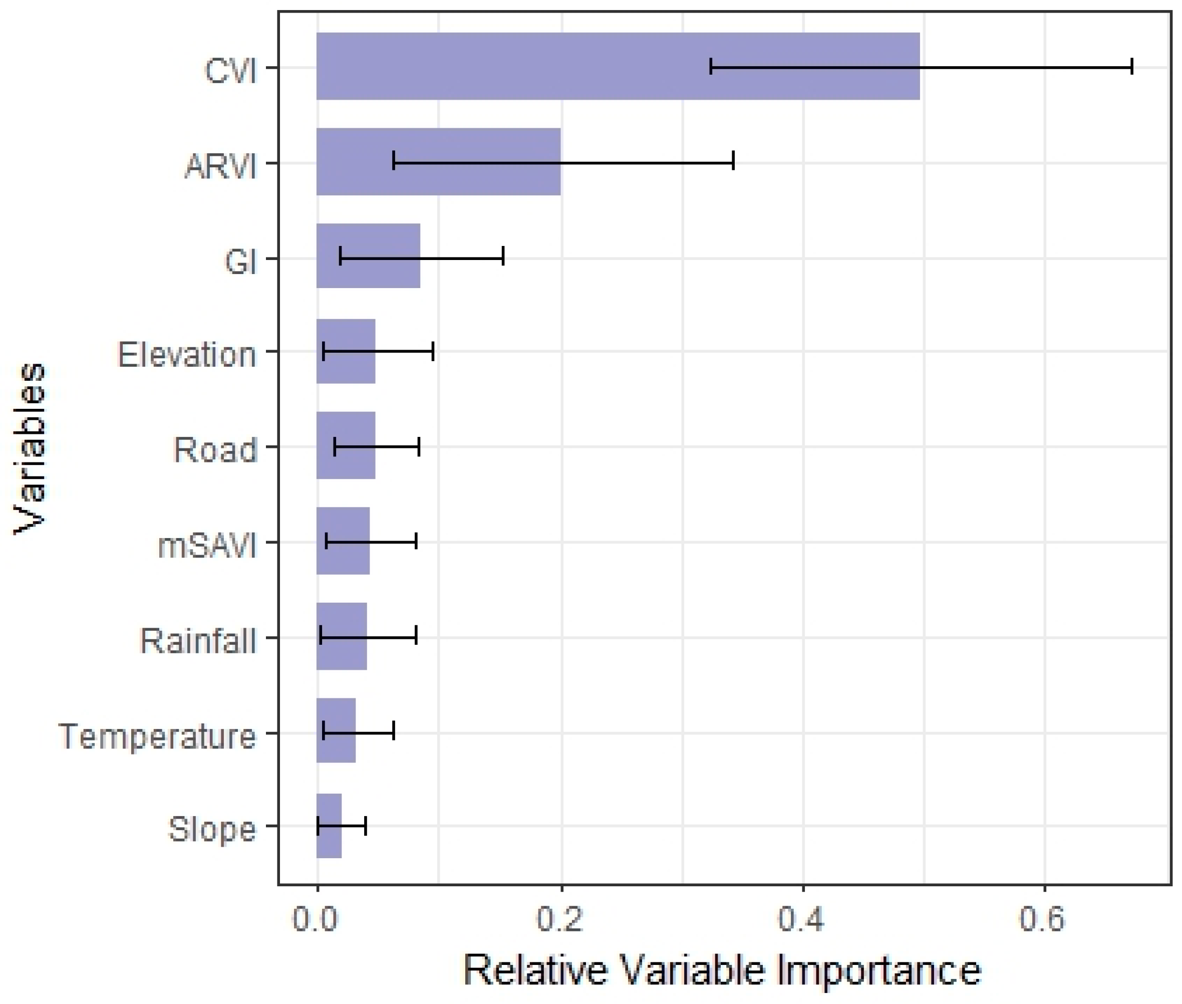
3.3. Variable Importance
4. Discussion
5. Conclusions
Author Contributions
Funding
Data Availability Statement
Acknowledgments
Conflicts of Interest
Appendix A
| No. | Name | Abbreviation | Formula |
| 1 | Atmospherically Resistant Vegetation Index | ARVI | |
| 2 | Blue Green Pigment Index | BGI | |
| 3 | Blue Normalized Difference Vegetation Index | BNDVI | |
| 4 | Chlorophyll Vegetation Index | CVI | |
| 5 | Difference Vegetation Index | DVI | |
| 6 | Differenced Vegetation Index MSS | DVIMSS | |
| 7 | Enhanced Vegetation Index | EVI | |
| 8 | Enhanced Vegetation Index 2 | EVI2 | |
| 9 | Green Atmospherically Resistant Vegetation Index | GARI | |
| 10 | Green-Blue NDVI | GBNDVI | |
| 11 | Greenness Index | GI | |
| 12 | Green Leaf Index | GLI | |
| 13 | Green NDVI | GNDVI | |
| 14 | Green Optimized SAVI | GOSAVI | |
| 15 | Green-Red NDVI | GRNDVI | |
| 16 | Green Ratio Vegetation Index | GRVI | |
| 17 | Infrared Percentage Vegetation Index | IPVI | |
| 18 | Leaf Area Index | LAI | |
| 19 | Modified NDVI | mNDVI | |
| 20 | Modified Simple Ratio | mSR | |
| 21 | Modified SAVI | mSAVI | |
| 22 | Normalized Difference Plant Pigment Ratio | PPR | |
| 23 | Normalized Difference Photosynthetic Vigor Ratio | PVR | |
| 24 | Normalized Difference 682/553 | ND682/553 | |
| 25 | Normalized Difference Vegetation Index | NDVI | |
| 26 | Red-Blue NDVI | RBNDVI | |
| 27 | Renormalized Difference Vegetation Index | RDVI | |
| 28 | Soil Adjusted Vegetation Index | SAVI | |
| 29 | Simple Ratio | SR | |
| 30 | Transformed NDVI | TNDVI | |
| 31 | Weighted Difference Vegetation Index | WDVI | |
| 32 | Wide Dynamic Range Vegetation Index | WDRVI | |
| where B is blue band, G is green band, R is red band, IR is infrared band, is 0.2, and is 0.5. | |||
References
- Stephens, S.S.; Wagner, M.R. Forest Plantations and Biodiversity: A Fresh Perspective. J. For. 2007, 105, 307–313. [Google Scholar]
- FAO. FAO Global Forest Resources Assessment 2020 Main Report; FAO: Rome, Germany, 2020; ISBN 9789251329740. [Google Scholar]
- Carnus, J.M.; Parrotta, J.; Brockerhoff, E.; Arbez, M.; Jactel, H.; Kremer, A.; Lamb, D.; O’Hara, K.; Walters, B. Planted Forests and Biodiversity. J. For. 2006, 104, 65–77. [Google Scholar]
- Pawson, S.M.; Brin, A.; Brockerhoff, E.G.; Lamb, D.; Payn, T.W.; Paquette, A.; Parrotta, J.A. Plantation Forests, Climate Change and Biodiversity. Biodivers. Conserv. 2013, 22, 1203–1227. [Google Scholar] [CrossRef]
- Paquette, A.; Hawryshyn, J.; Senikas, A.V.; Potvin, C. Enrichment Planting in Secondary Forests: A Promising Clean Development Mechanism to Increase Terrestrial Carbon Sinks. Ecol. Soc. 2009, 14, 31. [Google Scholar] [CrossRef]
- Van Der Meer, P.J.; Kanninen, M. Ecosystem Goods and Services from Plantation Forests. In Ecosystem Goods and Services from Plantation Forests; Routledge: Oxfordshire, UK, 2016. [Google Scholar]
- More, S.; Karpatne, A.; Wynne, R.H.; Thomas, V.A. Deep Learning for Forest Plantation Mapping in Godavari Districts of Andhra Pradesh, India. Earth Day KDD 2019, 1–5. Available online: https://vtechworks.lib.vt.edu/server/api/core/bitstreams/5da5a7e7-01e3-4546-a062-35f011047556/content (accessed on 8 June 2023).
- Brockerhoff, E.G.; Berndt, L.A.; Jactel, H. Role of Exotic Pine Forests in the Conservation of the Critically Endangered New Zealand Ground Beetle Holcaspis Brevicula (Coleoptera: Carabidae). N. Z. J. Ecol. 2005, 29, 37–43. [Google Scholar]
- Lemenih, M.; Kassa, H. Re-Greening Ethiopia: History, Challenges and Lessons. Forests 2014, 5, 1896–1909. [Google Scholar] [CrossRef]
- Bayle, G.K. Ecological and Social Impacts of Eucalyptus Tree Plantation on the Environment. J. Biodivers. Conserv. Bioresour. Manag. 2019, 5, 93–104. [Google Scholar] [CrossRef]
- Mekuria, W.; Wondie, M.; Amare, T.; Wubet, A.; Feyisa, T.; Yitaferu, B. Restoration of Degraded Landscapes for Ecosystem Services in North-Western Ethiopia. Heliyon 2018, 4, e00764. [Google Scholar] [CrossRef]
- Abiyu, A.; Teketay, D.; Gratzer, G.; Shete, M. Tree Planting by Smallholder Farmers in the Upper Catchment of Lake Tana Watershed, Northwest Ethiopia. Small Scale For. 2016, 15, 199–212. [Google Scholar] [CrossRef]
- Wondie, M.; Mekuria, W. Planting of Acacia Decurrens and Dynamics of Land Cover Change in Fagita Lekoma District in the Northwestern Highlands of Ethiopia. Mt. Res. Dev. 2018, 38, 230–239. [Google Scholar] [CrossRef]
- Tadesse, W.; Gezahgne, A.; Tesema, T.; Shibabaw, B. Plantation Forests in Amhara Region: Challenges and Best Measures for Future Improvements. World J. Agric. Res. 2019, 7, 149–157. [Google Scholar]
- Nambiar, E.S.; Harwood, C.E.; Kien, N.D. Acacia Plantations in Vietnam: Research and Knowledge Application to Secure a Sustainable Future. South. For. 2015, 77, 1–10. [Google Scholar] [CrossRef]
- Alemayehu, B. GIS and Remote Sensing Based Land Use/Land Cover Change Detection and Prediction in Fagita Lekoma Woreda, Awi Zone, Northwestern Ethiopia. Master’s Thesis, Addis Ababa University, Addis Ababa, Ethiopia, 2015; pp. 1–85. [Google Scholar]
- Berihun, M.L.; Tsunekawa, A.; Haregeweyn, N.; Meshesha, D.T.; Adgo, E.; Tsubo, M.; Masunaga, T.; Fenta, A.A.; Sultan, D.; Yibeltal, M. Exploring Land Use/Land Cover Changes, Drivers and Their Implications in Contrasting Agro-Ecological Environments of Ethiopia. Land Use Policy 2019, 87, 104052. [Google Scholar] [CrossRef]
- Baral, H.; Keenan, R.J.; Fox, J.C.; Stork, N.E.; Kasel, S. Spatial Assessment of Ecosystem Goods and Services in Complex Production Landscapes: A Case Study from South-Eastern Australia. Ecol. Complex. 2013, 13, 35–45. [Google Scholar] [CrossRef]
- Chazdon, R.L. Beyond Deforestation: Restoring Forests and Ecosystem Services on Degraded Lands. Science 2008, 320, 1458–1460. [Google Scholar] [CrossRef] [PubMed]
- Parrotta, J.A. The Role of Plantation Forests in Rehabilitating Degraded Tropical Ecosystems. Agric. Ecosyst. Environ. 1992, 41, 115–133. [Google Scholar] [CrossRef]
- Baillie, B.R.; Neary, D.G. Water Quality in New Zealand’s Planted Forests: A Review. N. Z. J. For. Sci. 2015, 45, 7. [Google Scholar] [CrossRef]
- Freer-smith, P. Plantation Forests: Potential and Impacts in Europe New EFI Study. 2019. Available online: https://efi.int/sites/default/files/files/thinkforest/2019/ThinkForest%20-%20Dec%202019_Freer-Smith.pdf (accessed on 12 June 2023).
- Akingbogun, A.; Kosoko, O.; Aborisade, D.K. Remote Sensing and GIS Application for Forest Reserve Degredation Prediction and Monitoring. In Proceedings of the FIG Young Surveyors Conference, Rome, Italy, 4–5 May 2012; pp. 1–27. [Google Scholar]
- Calders, K.; Jonckheere, I.; Nightingale, J.; Vastaranta, M. Remote Sensing Technology Applications in Forestry and REDD+. Forests 2020, 11, 188. [Google Scholar] [CrossRef]
- Lausch, A.; Erasmi, S.; King, D.J.; Magdon, P.; Heurich, M. Understanding Forest Health with Remote Sensing-Part I-A Review of Spectral Traits, Processes and Remote-Sensing Characteristics. Remote Sens. 2016, 8, 1029. [Google Scholar] [CrossRef]
- Liu, Q.; Zhang, S.; Zhang, H.; Bai, Y.; Zhang, J. Monitoring Drought Using Composite Drought Indices Based on Remote Sensing. Sci. Total Environ. 2020, 711, 134585. [Google Scholar] [CrossRef]
- Shahabi, H.; Shirzadi, A.; Ghaderi, K.; Omidvar, E.; Al-Ansari, N.; Clague, J.J.; Geertsema, M.; Khosravi, K.; Amini, A.; Bahrami, S.; et al. Flood Detection and Susceptibility Mapping Using Sentinel-1 Remote Sensing Data and a Machine Learning Approach: Hybrid Intelligence of Bagging Ensemble Based on K-Nearest Neighbor Classifier. Remote Sens. 2020, 12, 266. [Google Scholar] [CrossRef]
- Ahmed, N.; Atzberger, C.; Zewdie, W. Species Distribution Modelling Performance and Its Implication for Sentinel-2-Based Prediction of Invasive Prosopis Juliflora in Lower Awash River Basin, Ethiopia. Ecol. Process 2021, 10, 18. [Google Scholar] [CrossRef]
- de Simone, W.; Di Musciano, M.; Di Cecco, V.; Ferella, G.; Frattaroli, A.R. The Potentiality of Sentinel-2 to Assess the Effect of Fire Events on Mediterranean Mountain Vegetation. Plant Sociol. 2020, 57, 11–22. [Google Scholar] [CrossRef]
- Meng, Y.; Wei, C.; Guo, Y.; Tang, Z. A Planted Forest Mapping Method Based on Long-Term Change Trend Features Derived from Dense Landsat Time Series in an Ecological Restoration Region. Remote Sens. 2022, 14, 961. [Google Scholar] [CrossRef]
- Torbick, N.; Ledoux, L.; Salas, W.; Zhao, M. Regional Mapping of Plantation Extent Using Multisensor Imagery. Remote Sens. 2016, 8, 236. [Google Scholar] [CrossRef]
- Chi, H.; Sun, G.; Huang, J.; Guo, Z.; Ni, W.; Fu, A. National Forest Aboveground Biomass Mapping from ICESat/GLAS Data and MODIS Imagery in China. Remote Sens. 2015, 7, 5534–5564. [Google Scholar] [CrossRef]
- Fagan, M.E.; DeFries, R.S.; Sesnie, S.E.; Arroyo-Mora, J.P.; Soto, C.; Singh, A.; Townsend, P.A.; Chazdon, R.L. Mapping Species Composition of Forests and Tree Plantations in Northeastern Costa Rica with an Integration of Hyperspectral and Multitemporal Landsat Imagery. Remote Sens. 2015, 7, 5660–5696. [Google Scholar] [CrossRef]
- Frans, V.F.; Augé, A.A.; Fyfe, J.; Zhang, Y.; McNally, N.; Edelhoff, H.; Balkenhol, N.; Engler, J.O. Integrated SDM Database: Enhancing the Relevance and Utility of Species Distribution Models in Conservation Management. Methods Ecol. Evol. 2022, 13, 243–261. [Google Scholar] [CrossRef]
- Adem Esmail, B.; Geneletti, D. Multi-Criteria Decision Analysis for Nature Conservation: A Review of 20 Years of Applications. Methods Ecol. Evol. 2018, 9, 42–53. [Google Scholar] [CrossRef]
- Smeraldo, S.; Di Febbraro, M.; Ćirović, D.; Bosso, L.; Trbojević, I.; Russo, D. Species Distribution Models as a Tool to Predict Range Expansion after Reintroduction: A Case Study on Eurasian Beavers (Castor Fiber). J. Nat. Conserv. 2017, 37, 12–20. [Google Scholar] [CrossRef]
- Lorena, A.C.; Jacintho, L.F.O.; Siqueira, M.F.; Giovanni, R.D.; Lohmann, L.G.; De Carvalho, A.C.P.L.F.; Yamamoto, M. Comparing Machine Learning Classifiers in Potential Distribution Modelling. Expert. Syst. Appl. 2011, 38, 5268–5275. [Google Scholar] [CrossRef]
- Ortega-Huerta, M.A.; Peterson, A.T. Modelling Spatial Patterns of Biodiversity for Conservation Prioritization in North-Eastern Mexico. Divers. Distrib. 2004, 10, 39–54. [Google Scholar] [CrossRef]
- Angelieri, C.C.S.; Adams-Hosking, C.; Paschoaletto, K.M.; De Barros Ferraz, M.; De Souza, M.P.; McAlpine, C.A. Using Species Distribution Models to Predict Potential Landscape Restoration Effects on Puma Conservation. PLoS ONE 2016, 11, e0145232. [Google Scholar] [CrossRef]
- Schwartz, M.W. Using Niche Models with Climate Projections to Inform Conservation Management Decisions. Biol. Conserv. 2012, 155, 149–156. [Google Scholar] [CrossRef]
- Peterson, A.T.; Ortega-Huerta, M.A.; Bartley, J.; Sánchez-Cordero, V.; Soberón, J.; Buddemeler, R.H.; Stockwell, D.R.B. Future Projections for Mexican Faunas under Global Climate Change Scenarios. Nature 2002, 416, 626–629. [Google Scholar] [CrossRef]
- Rodríguez-Merino, A.; Fernández-Zamudio, R.; García-Murillo, P. An Invasion Risk Map for Non-Native Aquatic Macrophytes of the Iberian Peninsula. An. Del Jard. Bot. De Madr. 2017, 74, e055. [Google Scholar] [CrossRef]
- Cheung, W.W.L.; Rondinini, C.; Avtar, R.; van den Belt, M.; Hickler, T.; Metzger, J.P.; Scharlemann, J.P.W.; Velez-Liendo, X.; Yue, T.X. The Methodological Assessment Report on Scenarios and Models of Biodiversity and Ecosystem Services: Summary for Policymakers; IPBES: Bonn, Germany, 2016; ISBN 9789280735697. [Google Scholar]
- Elith, J.; Leathwick, J.R. Species Distribution Models: Ecological Explanation and Prediction across Space and Time. Annu. Rev. Ecol. Evol. Syst. 2009, 40, 677–697. [Google Scholar] [CrossRef]
- Guisan, A.; Thuiller, W.; Zimmermann, N.E. Habitat Suitability and Distribution Models; Cambridge University Press: Cambridge, UK, 2017. [Google Scholar]
- Václavík, T.; Meentemeyer, R.K. Invasive Species Distribution Modeling (ISDM): Are Absence Data and Dispersal Constraints Needed to Predict Actual Distributions? Ecol. Modell. 2009, 220, 3248–3258. [Google Scholar] [CrossRef]
- Marmion, M.; Parviainen, M.; Luoto, M.; Heikkinen, R.K.; Thuiller, W. Evaluation of Consensus Methods in Predictive Species Distribution Modelling. Divers. Distrib. 2009, 15, 59–69. [Google Scholar] [CrossRef]
- Amiri, M.; Tarkesh, M.; Shafiezadeh, M. Modelling the Biological Invasion of Prosopis Juliflora Using Geostatistical-Based Bioclimatic Variables under Climate Change in Arid Zones of Southwestern Iran. J. Arid. Land. 2022, 14, 203–224. [Google Scholar] [CrossRef]
- Arogoundade, A.M.; Odindi, J.; Mutanga, O. Modelling Parthenium Hysterophorus Invasion in KwaZulu-Natal Province Using Remotely Sensed Data and Environmental Variables. Geocarto Int. 2020, 35, 1450–1465. [Google Scholar] [CrossRef]
- Lesiv, M.; Laso Bayas, J.C.; See, L.; Duerauer, M.; Dahlia, D.; Durando, N.; Hazarika, R.; Kumar Sahariah, P.; Vakolyuk, M.; Blyshchyk, V.; et al. Estimating the Global Distribution of Field Size Using Crowdsourcing. Glob. Chang. Biol. 2019, 25, 174–186. [Google Scholar] [CrossRef]
- Rufin, P.; Bey, A.; Picoli, M.; Meyfroidt, P. Large-Area Mapping of Active Cropland and Short-Term Fallows in Smallholder Landscapes Using PlanetScope Data. Int. J. Appl. Earth Obs. Geoinf. 2022, 112, 102937. [Google Scholar] [CrossRef]
- Roy, D.P.; Huang, H.; Houborg, R.; Martins, V.S. A Global Analysis of the Temporal Availability of PlanetScope High Spatial Resolution Multi-Spectral Imagery. Remote Sens. Environ. 2021, 264, 112586. [Google Scholar] [CrossRef]
- Cui, B.; Huang, W.; Ye, H.; Chen, Q. The Suitability of PlanetScope Imagery for Mapping Rubber Plantations. Remote Sens. 2022, 14, 1061. [Google Scholar] [CrossRef]
- Csillik, O.; Kumar, P.; Asner, G.P. Challenges in Estimating Tropical Forest Canopy Height from Planet Dove Imagery. Remote Sens. 2020, 12, 1160. [Google Scholar] [CrossRef]
- Gargiulo, J.; Clark, C.; Lyons, N.; de Veyrac, G.; Beale, P.; Garcia, S. Spatial and Temporal Pasture Biomass Estimation Integrating Electronic Plate Meter, Planet Cubesats and Sentinel-2 Satellite Data. Remote Sens. 2020, 12, 3222. [Google Scholar] [CrossRef]
- Kimm, H.; Guan, K.; Jiang, C.; Peng, B.; Gentry, L.F.; Wilkin, S.C.; Wang, S.; Cai, Y.; Bernacchi, C.J.; Peng, J.; et al. Deriving High-Spatiotemporal-Resolution Leaf Area Index for Agroecosystems in the U.S. Corn Belt Using Planet Labs CubeSat and STAIR Fusion Data. Remote Sens. Environ. 2020, 239, 111615. [Google Scholar] [CrossRef]
- Skakun, S.; Kalecinski, N.I.; Brown, M.G.L.; Johnson, D.M.; Vermote, E.F.; Roger, J.C.; Franch, B. Assessing Within-Field Corn and Soybean Yield Variability from Worldview-3, Planet, Sentinel-2, and Landsat 8 Satellite Imagery. Remote Sens. 2021, 13, 872. [Google Scholar] [CrossRef]
- Jin, Y.; Guo, J.; Ye, H.; Zhao, J.; Huang, W.; Cui, B. Extraction of Arecanut Planting Distribution Based on the Feature Space Optimization of Planetscope Imagery. Agriculture 2021, 11, 371. [Google Scholar] [CrossRef]
- Kaky, E.; Nolan, V.; Alatawi, A.; Gilbert, F. A Comparison between Ensemble and MaxEnt Species Distribution Modelling Approaches for Conservation: A Case Study with Egyptian Medicinal Plants. Ecol. Inform. 2020, 60, 101150. [Google Scholar] [CrossRef]
- Parrotta, J.A.; Turnbull, J.W.; Jones, N. Introduction Catalyzing Native Forest Regeneration on Degraded Tropical Lands. For. Ecol. Manag. 1997, 99, 1–7. [Google Scholar] [CrossRef]
- Barrio-Anta, M.; Castedo-Dorado, F.; Cámara-Obregón, A.; López-Sánchez, C.A. Integrating Species Distribution Models at Forest Planning Level to Develop Indicators for Fast-Growing Plantations. A Case Study of Eucalyptus Globulus Labill. in Galicia (NW Spain). For. Ecol. Manage 2021, 491, 119200. [Google Scholar] [CrossRef]
- Teshome, T.; Wondimu, A. Best Practices on Development and Utilatation of Acacia Decurrens in Fagta Lekoma District, Awi Zone, Amhara Region. 2019, 37. Available online: https://www.epa.gov.et/images/PDF/ForestManuals/BEST%20PRACTICES%20ON%20DEVELOPMENT%20AND%20UTILIZATION%20OF%20ACACIA%20DECURRENS.pdf (accessed on 7 January 2022).
- Worku, T.; Mekonnen, M.; Yitaferu, B.; Cerdà, A. Conversion of Crop Land Use to Plantation Land Use, Northwest Ethiopia. Trees For. People 2021, 3, 100044. [Google Scholar] [CrossRef]
- Keneni, Y.G.; Senbeta, A.F.; Sime, G. Role of small-scale trees plantation and farmers’ attitude and skill toward propagation of indigenous and exotic trees: The case of Sidama, Ethiopia. Afr. J. Food Agric. Nutr. Dev. 2021, 21, 18804–18823. [Google Scholar] [CrossRef]
- Yibeltal, M.; Tsunekawa, A.; Haregeweyn, N.; Adgo, E.; Meshesha, D.T.; Aklog, D.; Masunaga, T.; Tsubo, M.; Billi, P.; Vanmaercke, M.; et al. Analysis of Long-Term Gully Dynamics in Different Agro-Ecology Settings. Catena 2019, 179, 160–174. [Google Scholar] [CrossRef]
- Bazie, Z.; Feyssa, S.; Amare, T. Effects of Acacia Decurrens Willd. Tree-Based Farming System on Soil Quality in Guder Watershed, North Western Highlands of Ethiopia. Cogent Food Agric. 2020, 6, 1743622. [Google Scholar] [CrossRef]
- Chanie, Y.; Abewa, A. Expansion of Acacia Decurrens Plantation on the Acidic Highlands of Awi Zone, Ethiopia, and Its Socio-Economic Benefits. Cogent Food Agric. 2021, 7, 1917150. [Google Scholar] [CrossRef]
- Alemayehu, B.; Suarez-Minguez, J.; Rosette, J.; Khan, S.A. Vegetation Trend Detection Using Time Series Satellite Data as Ecosystem Condition Indicators for Analysis in the Northwestern Highlands of Ethiopia. Remote Sens. 2023, 15, 5032. [Google Scholar] [CrossRef]
- Harrison, T.N. Introduction to Planet’s New 8-Band Data and Access via NASA’s Commercial SmallSat Data Acquisition (CSDA) Program. 2022. Available online: https://www.earthdata.nasa.gov/s3fs-public/2022-06/PlanetCSDA8-Band_Data_0.pdf (accessed on 23 August 2023).
- Lottering, R.; Mutanga, O.; Peerbhay, K. Detecting and Mapping Levels of Gonipterus Scutellatus-Induced Vegetation Defoliation and Leaf Area Index Using Spatially Optimized Vegetation Indices. Geocarto Int. 2018, 33, 277–292. [Google Scholar] [CrossRef]
- Dong, J.; Zhou, C.; Liang, W.; Lu, X. Determination Factors for the Spatial Distribution of Forest Cover: A Case Study of China’s Fujian Province. Forests 2022, 13, 2070. [Google Scholar] [CrossRef]
- Shunlin Liang, J.W. Forest Cover Changes. In Advanced Remote Sensing; Elsevier: Amsterdam, The Netherlands, 2020; pp. 915–952. ISBN 9780128158265. [Google Scholar]
- Singh, S. Understanding the Role of Slope Aspect in Shaping the Vegetation Attributes and Soil Properties in Montane Ecosystems. Trop. Ecol. 2018, 59, 417–430. [Google Scholar]
- Xie, C.; Li, M.; Jim, C.Y.; Liu, D. Environmental Factors Driving the Spatial Distribution Pattern of Venerable Trees in Sichuan Province, China. Plants 2022, 11, 3581. [Google Scholar] [CrossRef]
- Agujetas Perez, M.; Tegebu, F.N.; Steenbergen, F. van Roadside Planting in Ethiopia: Turning a Problem into an Opportunity. Sustain. Environ. 2016, 1, 98. [Google Scholar] [CrossRef]
- Stage, A.R.; Salas, C. Interactions of Elevation, Aspect, and Slope in Models of Forest Species Composition and Productivity. For. Sci. 2007, 53, 486–492. [Google Scholar]
- Zhang, X.N.; Yang, X.D.; Li, Y.; He, X.M.; Lv, G.H.; Yang, J.J. Influence of Edaphic Factors on Plant Distribution and Diversity in the Arid Area of Xinjiang, Northwest China. Arid Land Res. Manag. 2018, 32, 38–56. [Google Scholar] [CrossRef]
- Naimi, B.; Hamm, N.A.S.; Groen, T.A.; Skidmore, A.K.; Toxopeus, A.G. Where Is Positional Uncertainty a Problem for Species Distribution Modelling? Ecography 2014, 37, 191–203. [Google Scholar] [CrossRef]
- Adeyemo, S.M.; Granger, J.J. Habitat Suitability Model and Range Shift Analysis for American Chestnut (Castanea Dentata) in the United States. Trees For. People 2023, 11, 100360. [Google Scholar] [CrossRef]
- Naimi, B.; Araújo, M.B. Sdm: A Reproducible and Extensible R Platform for Species Distribution Modelling. Ecography 2016, 39, 368–375. [Google Scholar] [CrossRef]
- Cheek, P.J.; McCullagh, P.; Nelder, J.A. Generalized Linear Models, 2nd ed.; Applied Statistics; Routledge: Oxfordshire, UK, 1990; Volume 39, p. 385. [Google Scholar]
- Friedman, J.H. Multivariate Adaptive Regression Splines. Ann. Stat. 2007, 19, 1–67. [Google Scholar] [CrossRef]
- Friedman, J.H. Greedy Function Approximation: A Gradient Boosting Machine. Ann. Stat. 2001, 29, 1189–1232. [Google Scholar] [CrossRef]
- Breiman, L. Random Forests; University of California: Oakland, CA, USA, 2001; Volume 7, pp. 1–33. [Google Scholar] [CrossRef]
- Vapnik, V.N. The Nature of Statistical Learning Theory; Springer: New York, NY, USA, 2000; ISBN 978-1-4419-3160-3. [Google Scholar]
- Breiman, L.; Friedman, J.H.; Olshen, R.A.; Stone, C.J. Classification and Regression Trees; 1984; ISBN 9780412048418. Available online: https://rafalab.dfci.harvard.edu/pages/649/section-11.pdf (accessed on 19 May 2023).
- Araújo, M.B.; New, M. Ensemble Forecasting of Species Distributions. Trends Ecol. Evol. 2007, 22, 42–47. [Google Scholar] [CrossRef]
- Pecchi, M.; Marchi, M.; Burton, V.; Giannetti, F.; Moriondo, M.; Bernetti, I.; Bindi, M.; Chirici, G. Species Distribution Modelling to Support Forest Management. A Literature Review. Ecol. Modell. 2019, 411, 108817. [Google Scholar] [CrossRef]
- Thuiller, W.; Lafourcade, B.; Engler, R.; Araújo, M.B. BIOMOD—A Platform for Ensemble Forecasting of Species Distributions. Ecography 2009, 32, 369–373. [Google Scholar] [CrossRef]
- Araújo, M.B.; Pearson, R.G.; Thuiller, W.; Erhard, M. Validation of Species-Climate Impact Models under Climate Change. Glob. Chang. Biol. 2005, 11, 1504–1513. [Google Scholar] [CrossRef]
- Fielding, A.H.; Bell, J.F. A Review of Methods for the Assessment of Prediction Errors in Conservation Presence/Absence Models. Environ. Conserv. 1997, 24, 38–49. [Google Scholar] [CrossRef]
- Allouche, O.; Tsoar, A.; Kadmon, R. Assessing the Accuracy of Species Distribution Models: Prevalence, Kappa and the True Skill Statistic (TSS). J. Appl. Ecol. 2006, 43, 1223–1232. [Google Scholar] [CrossRef]
- Jiménez-Valverde, A. Insights into the Area under the Receiver Operating Characteristic Curve (AUC) as a Discrimination Measure in Species Distribution Modelling. Glob. Ecol. Biogeogr. 2012, 21, 498–507. [Google Scholar] [CrossRef]
- Zhang, L.; Liu, S.; Sun, P.; Wang, T.; Wang, G.; Zhang, X.; Wang, L. Consensus Forecasting of Species Distributions: The Effects of Niche Model Performance and Niche Properties. PLoS ONE 2015, 10, e0120056. [Google Scholar] [CrossRef]
- Duque-Lazo, J.; van Gils, H.; Groen, T.A.; Navarro-Cerrillo, R.M. Transferability of Species Distribution Models: The Case of Phytophthora Cinnamomi in Southwest Spain and Southwest Australia. Ecol. Modell. 2016, 320, 62–70. [Google Scholar] [CrossRef]
- De Marco, P.; Nóbrega, C.C. Evaluating Collinearity Effects on Species Distribution Models: An Approach Based on Virtual Species Simulation. PLoS ONE 2018, 13, e0202403. [Google Scholar] [CrossRef]
- Chatterjee, S.; Hadi, A.S. Regression-Analysis-by-Example; Wiley: Hoboken, NJ, USA, 2012; pp. 1–421. [Google Scholar]
- Dormann, C.F.; Elith, J.; Bacher, S.; Buchmann, C.; Carl, G.; Carré, G.; Marquéz, J.R.G.; Gruber, B.; Lafourcade, B.; Leitão, P.J.; et al. Collinearity: A Review of Methods to Deal with It and a Simulation Study Evaluating Their Performance. Ecography 2013, 36, 27–46. [Google Scholar] [CrossRef]
- Engler, R.; Waser, L.T.; Zimmermann, N.E.; Schaub, M.; Berdos, S.; Ginzler, C.; Psomas, A. Combining Ensemble Modeling and Remote Sensing for Mapping Individual Tree Species at High Spatial Resolution. For. Ecol. Manage 2013, 310, 64–73. [Google Scholar] [CrossRef]
- Li, J. Assessing the Accuracy of Predictive Models for Numerical Data: Not r nor R2, Why Not? Then What? PLoS ONE 2017, 12, e0183250. [Google Scholar] [CrossRef]
- Maxwell, A.E.; Sharma, M.; Donaldson, K.A. Explainable Boosting Machines for Slope Failure Spatial Predictive Modeling. Remote Sens. 2021, 13, 4991. [Google Scholar] [CrossRef]
- González-Irusta, J.M.; González-Porto, M.; Sarralde, R.; Arrese, B.; Almón, B.; Martín-Sosa, P. Comparing Species Distribution Models: A Case Study of Four Deep Sea Urchin Species. Hydrobiologia 2015, 745, 43–57. [Google Scholar] [CrossRef]
- Qiao, H.; Soberón, J.; Peterson, A.T. No Silver Bullets in Correlative Ecological Niche Modelling: Insights from Testing among Many Potential Algorithms for Niche Estimation. Methods Ecol. Evol. 2015, 6, 1126–1136. [Google Scholar] [CrossRef]
- Mugo, R.; Saitoh, S.-I. Ensemble Modelling of Skipjack Tuna (Katsuwonus pelamis) Habitats in the Western North Pacific Using Satellite Remotely Sensed Data; a Comparative Analysis Using Machine-Learning Models. Remote Sens. 2020, 12, 2591. [Google Scholar] [CrossRef]
- Montoya-Jiménez, J.C.; Valdez-Lazalde, J.R.; Ángeles-Perez, G.; de los SantosPosadas, H.M.; Cruz-Cárdenas, G. Predictive Capacity of Nine Algorithms and an Ensemble Model to Determine the Geographic Distribution of Tree Species. IForest 2022, 15, 363–371. [Google Scholar] [CrossRef]
- Talukdar, S.; Singha, P.; Mahato, S.; Shahfahad; Pal, S.; Liou, Y.A.; Rahman, A. Land-Use Land-Cover Classification by Machine Learning Classifiers for Satellite Observations-A Review. Remote Sens. 2020, 12, 1135. [Google Scholar] [CrossRef]
- Rodriguez-Galiano, V.F.; Ghimire, B.; Rogan, J.; Chica-Olmo, M.; Rigol-Sanchez, J.P. An Assessment of the Effectiveness of a Random Forest Classifier for Land-Cover Classification. ISPRS J. Photogramm. Remote Sens. 2012, 67, 93–104. [Google Scholar] [CrossRef]
- Hassan, C.A.; Khan, M.S.; Shah, M.A. Comparison of Machine Learning Algorithms in Data Classification. In Proceedings of the ICAC 2018—2018 24th IEEE International Conference on Automation and Computing: Improving Productivity through Automation and Computing, Newcastle Upon Tyne, UK, 6–7 September 2018; Institute of Electrical and Electronics Engineers Inc.: Piscataway, NJ, USA, 2018. [Google Scholar]
- Elith, J.; Leathwick, J.R.; Hastie, T. A Working Guide to Boosted Regression Trees. J. Anim. Ecol. 2008, 77, 802–813. [Google Scholar] [CrossRef]
- Cheng, L.; Lek, S.; Lek-Ang, S.; Li, Z. Predicting Fish Assemblages and Diversity in Shallow Lakes in the Yangtze River Basin. Limnologica 2012, 42, 127–136. [Google Scholar] [CrossRef]
- He, Y.; Wang, J.; Lek-Ang, S.; Lek, S. Predicting Assemblages and Species Richness of Endemic Fish in the Upper Yangtze River. Sci. Total Environ. 2010, 408, 4211–4220. [Google Scholar] [CrossRef]
- Grenouillet, G.; Buisson, L.; Casajus, N.; Lek, S. Ensemble Modelling of Species Distribution: The Effects of Geographical and Environmental Ranges. Ecography 2011, 34, 9–17. [Google Scholar] [CrossRef]
- Makhkamov, T.K.; Brundu, G.; Jabborov, A.M.; Gaziev, A.D. Predicting the Potential Distribution of Ranunculus Sardous (Ranunculaceae), a New Alien Species in the Flora of Uzbekistan and Central Asia. Bioinvasions Rec. 2023, 12, 63–77. [Google Scholar] [CrossRef]
- Aguirre-Gutiérrez, J.; Carvalheiro, L.G.; Polce, C.; van Loon, E.E.; Raes, N.; Reemer, M.; Biesmeijer, J.C. Fit-for-Purpose: Species Distribution Model Performance Depends on Evaluation Criteria—Dutch Hoverflies as a Case Study. PLoS ONE 2013, 8, e63708. [Google Scholar] [CrossRef]
- Yuan, J.; Wu, Z.; Li, S.; Kang, P.; Zhu, S. Multi-Feature-Based Identification of Subtropical Evergreen Tree Species Using Gaofen-2 Imagery and Algorithm Comparison. Forests 2023, 14, 292. [Google Scholar] [CrossRef]
- Anna, C. Potential of Multi-Temporal Remote Sensing Data for Modeling Tree Species Distributions and Species Richness in Mexico; Institute for Geography and Geology, Julius Maximilian University of Würzburg: Wuerzburg, Germany, 2012. [Google Scholar]
- Wen, L.; Saintilan, N.; Yang, X.; Hunter, S.; Mawer, D. MODIS NDVI Based Metrics Improve Habitat Suitability Modelling in Fragmented Patchy Floodplains. Remote Sens. Appl. 2015, 1, 85–97. [Google Scholar] [CrossRef]
- Nogués-Bravo, D.; Araújo, M.B.; Romdal, T.; Rahbek, C. Scale Effects and Human Impact on the Elevational Species Richness Gradients. Nature 2008, 453, 216–219. [Google Scholar] [CrossRef]
- Muche, M.; Molla, E.; Rewald, B.; Tsegay, B.A. Diversity and Composition of Farm Plantation Tree/Shrub Species along Altitudinal Gradients in North-Eastern Ethiopia: Implication for Conservation. Heliyon 2022, 8, e09048. [Google Scholar] [CrossRef] [PubMed]
- Thaiutsa, B.C. Commercial Plantation in Thailand: A Case Study of the Forest Industry Organization. In Proceedings of the FORTROP II: Tropical Forestry Change in a Changing World, Bangkok, Thailand, 17–20 November 2008. [Google Scholar]
- Altamirano, A.; Lara, A. Deforestación En Ecosistemas Templados de La Precordillera Andina Del Centro-Sur de Chile. Bosque 2010, 31, 53–64. [Google Scholar] [CrossRef]
- Kaczan, D.J. Can Roads Contribute to Forest Transitions? Duke University: Durham, NC, USA, 2017. [Google Scholar]


| No. | Variables | VIF |
|---|---|---|
| 1 | ARVI | 7.414995 |
| 2 | Aspect | 1.190828 |
| 3 | CVI | 6.169403 |
| 4 | Elevation | 3.323751 |
| 5 | GI | 3.797256 |
| 6 | mSAVI | 3.771155 |
| 7 | Rainfall | 3.080133 |
| 8 | Road | 1.192230 |
| 9 | Slope | 1.220056 |
| 10 | Soil type | 1.724052 |
| 11 | Temperature | 5.638469 |
| Algorithm | AUC | Sensitivity | Specificity | TSS |
|---|---|---|---|---|
| GLM | 0.84 | 0.81 | 0.83 | 0.64 |
| MARS | 0.85 | 0.82 | 0.83 | 0.65 |
| BRT | 0.89 | 0.83 | 0.87 | 0.7 |
| RF | 0.93 | 0.9 | 0.92 | 0.82 |
| SVM | 0.89 | 0.82 | 0.89 | 0.71 |
| CART | 0.84 | 0.8 | 0.85 | 0.65 |
Disclaimer/Publisher’s Note: The statements, opinions and data contained in all publications are solely those of the individual author(s) and contributor(s) and not of MDPI and/or the editor(s). MDPI and/or the editor(s) disclaim responsibility for any injury to people or property resulting from any ideas, methods, instructions or products referred to in the content. |
© 2024 by the authors. Licensee MDPI, Basel, Switzerland. This article is an open access article distributed under the terms and conditions of the Creative Commons Attribution (CC BY) license (https://creativecommons.org/licenses/by/4.0/).
Share and Cite
Alemayehu, B.; Suarez-Minguez, J.; Rosette, J. Modeling the Spatial Distribution of Acacia decurrens Plantation Forests Using PlanetScope Images and Environmental Variables in the Northwestern Highlands of Ethiopia. Forests 2024, 15, 277. https://doi.org/10.3390/f15020277
Alemayehu B, Suarez-Minguez J, Rosette J. Modeling the Spatial Distribution of Acacia decurrens Plantation Forests Using PlanetScope Images and Environmental Variables in the Northwestern Highlands of Ethiopia. Forests. 2024; 15(2):277. https://doi.org/10.3390/f15020277
Chicago/Turabian StyleAlemayehu, Bireda, Juan Suarez-Minguez, and Jacqueline Rosette. 2024. "Modeling the Spatial Distribution of Acacia decurrens Plantation Forests Using PlanetScope Images and Environmental Variables in the Northwestern Highlands of Ethiopia" Forests 15, no. 2: 277. https://doi.org/10.3390/f15020277