Quantifying Forest Cover Loss as a Response to Drought and Dieback of Norway Spruce and Evaluating Sensitivity of Various Vegetation Indices Using Remote Sensing

Abstract

The Norway spruce is one of the most important tree species in Europe. This tree species has been put under considerable pressure due to the ongoing impacts of climate change. Meanwhile, frequent droughts and pest outbreaks are reported as the main reason for its dieback, resulting in severe forest cover loss. Such was the case with Norway spruce forests within the Kopaonik National Park (NP) in Serbia. This study aims to quantify, spatially and temporally, forest cover loss and to evaluate the sensitivity of various vegetation indices (VIs) in detecting drought-induced response and predicting the dieback of Norway spruce due to long-lasting drought effects in the Kopaonik NP. For this purpose, we downloaded and processed a large number of Landsat 7 (ETM+), Landsat 8 (OLI), and Sentinel 2 (MSI) satellite imagery acquired from 2009 to 2022. Our results revealed that forest cover loss was mainly driven by severe drought in 2011 and 2012, which was later significantly influenced by bark beetle outbreaks. Furthermore, various VIs proved to be very useful in monitoring and predicting forest health status. In summary, the drought-induced response detected using various VIs provides valuable insights into the dynamics of forest cover change, with implications for monitoring and conservation efforts of Norway spruce forests in the Kopaonik NP.

1. Introduction

In Europe (excluding Russia), from 1990 to 2020, according to GFRA 2020 (Global Forest Resources Assessment), the area under forest increased by about 17 million ha, while in certain areas of Europe, the process of deforestation has been more evident in recent years [1]. In this context, due to various disturbances, such as adverse climate events, insect pests, epiphytocia, etc., one of the most endangered species in Europe is Norway spruce (Picea abies (L.) Karst.) [2,3,4,5,6,7,8]. This is very important as Norway spruce, from an ecological and economic point of view, is one of Europe’s most important conifer species. It can be found in various areas, occurring from the boreal forests in Northern Europe to subalpine areas of the Alps and the Carpathian Mountains [9]. In the Balkans, unlike the rest of Europe, Norway spruce rarely occurs at lower altitudes, and it is usually found in high mountains and mountain ranges where the climate is cold and humid [10]. In general, the share of conifers in Serbia is relatively small, consisting of 12% of the total forest stand volume, whereas Norway spruce is the most dominant species with a share of 5.2% [11]. Naturally, Norway spruce is dominantly distributed in southwestern Serbia, found in the Tara, Zlatar, Golija, Kopaonik, Mokra Gora, Murtenica (Zlatibor), Radočelo, Prokletije, and Šar Planina mountains, and several other smaller mountain massifs near the Montenegro border, most commonly in suitable climatic, orographic and edaphic conditions [12]. The exception is its presence in the Stara Planina mountain, near the Bulgaria border in southeastern Serbia.

Numerous European studies have pointed out that Norway spruce is a species that is particularly sensitive to drought, especially dry and hot summers [13,14,15,16,17,18,19,20,21,22,23,24,25,26,27]. It is important to note that in the Balkans, few studies on this topic have been carried out, and in Norway, spruce stands [28,29,30,31]. However, in recent years, as a result of extreme climatic events, such as drought, the dieback of Norway spruce has been reported locally in Serbia [30,31,32,33] and regionally in Croatia [7], Bosnia and Herzegovina [34,35,36], and Montenegro [32]. Considering that the research projections of Miletić et al. [37] suggest that the climate in vast areas of Serbia, by the middle and, especially, the end of the 21st century, may be unfavorable for Norway spruce, we can only expect that devitalization and dieback of trees may occur more often and with greater intensity.

Devitalization and dieback of Norway spruce trees, the most important species at the Kopaonik National Park (NP), is a process that, sporadically, lasts for many years. However, significant dieback of Norway spruce trees was noted as a result of severe drought in 2011, especially in 2012, and bark beetle outbreaks in 2015 and 2016, until today. In the first years of this period, dieback occurred in individual trees and small groups; however, since that time, dieback has been reported in large groups and entire stands of Norway spruce [38].

In the last decade, such events have often been studied with the use of remote sensing-produced vegetation indices (VIs) to provide precise explanations of spatial–temporal trends of drought effects [4,38,39,40,41], pest outbreaks [42,43,44,45,46,47,48], and other forest disturbances [42,43,44,45]. By utilizing the spectral reflectance characteristics of plants, gathered via various imaging techniques, and combining reflectance from specific spectral wavelengths (bands) [49], VIs make the large-scale analysis of forest vegetation inexpensive and reliable. As proven by many studies [43,45,50,51,52,53], VIs have also been found to be very sensitive in forecasting conifer health status, as they can signal drought stress and pest outbreaks, facilitating timely interventions in forest management and thus reducing the adverse effects of such disturbances. Therefore, the non-invasive approach and efficiency of VIs in forest health monitoring, which is made possible using high temporal frequency and spatially explicit satellite data, can provide insights into current and future forest health status over large-scale forested areas. For example, various VIs have been applied in forest health monitoring, and the most common ones are the Normalized Difference Vegetation Index (NDVI), the Soil-Adjusted Vegetation Index (SAVI), the Transformed Vegetation Index (TVI), the Normalized Difference Moisture Index (NDMI), the Disease Water Stress Index (DSWI), Tasseled Cap Wetness (TCW), and Tasseled Cap Greenness (TCG) [38,39,45,46,47,48,50,53,54,55,56]. Despite their high accuracy, other conventional methods require constant, time-consuming, and cost-ineffective monitoring service, thus indicating the utter importance and innovativeness of remote sensing-produced VIs in monitoring forest health status over large-scale forested areas. Regardless, the application of VIs has not demonstrated any significant use in forest-themed studies in Serbia. Past studies in Serbia have mainly focused on spatial and temporal forest cover mapping [57,58,59,60,61,62,63], mapping of illegal logging effects [64,65], and mapping of wildfire effects [66,67]. An exception is the research of Jovanović and Milanović [68], in which the health status of beech forests was evaluated using VIs, more precisely the NDVI. As past studies in Serbia did not provide precise answers for drought-induced causes or other causes of deforestation, in this research, we aim to fill those gaps by quantifying, spatially and temporally, forest cover loss and evaluating the sensitivity of several VIs in detecting responses to drought and predicting the dieback of Norway spruce due to long-lasting drought effects in the Kopaonik NP. Based on our research goals, we formulated two hypotheses:

Hypothesis 1 (H1). 

There is a significant relationship between drought-induced dieback of Norway spruce and forest cover loss.

Hypothesis 2 (H2). 

Different VIs showed varying levels of sensitivity in the prediction of drought-induced dieback of Norway spruce, with some VIs providing more accurate prediction of forest cover loss than others.

2. Materials and Methods

2.1. Study Area

The study area (Figure 1) is situated within the Kopaonik National Park (NP) in southern Serbia, which gained its current status in the year 1981 due to its biodiversity, rich flora and fauna, and great cultural and historical importance [69,70]. The park stretches across 11,969.04 ha of land in low-populated areas of municipalities Brus and Raška, mainly on mountain Kopaonik (2017 m.a.s.l) [71,72], of which 7427.24 ha is covered by forests [73]. Higher parts of the mountain are mainly covered with pure or mixed conifer stands of Norway spruce (Picea abies (L.) Karst.) and Silver fir (Abies alba (L.) Mill.), with or without European beech (Fagus sylvatica L.), which in addition to Austrian pine (Pinus nigra Arn.) and oak species (Quercus spp.), dominates the lower parts of the mountain [73]. Such species distribution is mainly driven by the wide altitudinal range, namely by site-specific ecological conditions of different altitude levels. Generally, the climate in the Kopaonik NP is characterized as subalpine [70], with an average annual temperature of 4.1 °C and an average annual precipitation of 1040.1 mm (climatic sequence 1991–2020) [74]. By comparing the last two climatic sequences (1961–1990 and 1991–2020), it can be found that the average annual temperature in the Kopaonik NP increased by 1.4 °C, and the average annual precipitation increased by 119.3 mm [75]. As significant devitalization and dieback of trees are reported more frequently in pure stands and less in mixed stands of Norway spruce, we narrowed the research area down to 2385.72 ha of such forests, using forestry stand maps provided by the Kopaonik NP. A major component of the research area is located in the area under the protection regime of the second degree, where, according to Đorđević et al. [73], limited and strictly controlled use of natural resources and activities is established to the extent that it does not endanger natural habitats.

2.2. Data Collection

To evaluate the impact of drought on the forest cover loss at Mt. Kopaonik (Appendix A), we downloaded Landsat 7 (ETM+), Landsat 8 (OLI) Level 1, and Sentinel-2A/2B (MSI) Level 1C satellite imagery (from 2009 to 2022) using the U.S. Geological Survey Earth Explorer website (https://earthexplorer.usgs.gov, accessed 11 January 2024) and the Semi-Automatic Classification v.7.10.11-Matera (SCP) plugin [76] from the QGIS v.3.22.6 Białowieża (OSGeo, Chicago, IL, US) software (

Table 1. The imagery used for the evaluation of drought effects on the forest cover loss.

Sensor	Date Acquired	Path/Row
Landsat 7	22 August 2009	186/030
Landsat 7	21 July 2009	186/030
Landsat 7	19 June 2009	186/030
Landsat 7	21 August 2011	185/030
Landsat 7	27 July 2011	186/030
Landsat 7	12 August 2011	186/030
Landsat 7	28 August 2011	186/030
Landsat 7	23 August 2012	185/030
Landsat 7	29 July 2012	186/030
Landsat 7	14 August 2012	186/030
Landsat 7	30 August 2012	186/030
Landsat 8	01 July 2013	185/030
Landsat 8	25 August 2013	186/030
Landsat 8	28 August 2014	186/030
Landsat 8	09 August 2013	186/030
Landsat 8	12 August 2014	186/030

and

Table 2. The imagery used for mapping forest cover loss.

Sensor	Date Acquired	Path/Row
Landsat 8	09 August 2013	186/030
Landsat 8	12 August 2014	186/030
Sentinel 2	31 August 2015	136 *
Sentinel 2	15 August 2016	136 *
Sentinel 2	11 July 2017	136 *
Sentinel 2	21 July 2018	136 *
Sentinel 2	01 July 2019	136 *
Sentinel 2	29 August 2020	136 *
Sentinel 2	25 July 2021	136 *
Sentinel 2	20 July 2022	136 *

* Relative orbit number (Sentinel 2).

). The 2009 to 2022 time period was selected to ensure that the state of vegetation in pre-drought (2009), drought (2011 and 2012), and post-drought (2013–2022) periods when severe pest outbreaks occurred was analyzed in order to obtain a complete picture of how Norway spruce is responding to the adverse effects of climate change. We selected only the cloud-free imagery acquired during the growing season, which, in our case, included imagery acquired only in July and August (except for one image from June). The 2010 imagery was not downloaded because, in all available Landsat 7 (ETM+) data, the images covering most of our research area were covered with clouds.

2.3. Data Processing

The downloaded Landsat 7 (ETM+) and Landsat 8 (OLI) MS bands, R, G, B, NIR, SWIR1, and SWIR2, including Sentinel-2 (MSI) Level-1C MS bands, B, G, R, VRE, VRE2, VRE3, NIR, NIR2, SWIR2, and SWIR3, were automatically processed using the SCP plugin by converting them from DN [Landsat] and scaled top of atmosphere (TOA) reflectance [Sentinel] into the TOA reflectance to reduce the inter-scene variability through a normalization for solar irradiance. Atmospheric correction of all images was carried out using an image-based technique called Dark Object Subtraction (DOS1) [77], as cited in [76]. Ordinary least squares regression (OLS) equations from Roy et al. [78] were used to normalize the reflectance of one Landsat sensor to the other (ETM+ to OLI). Before applying the pan-sharpening Brovey Transform technique [79] using the SCP plugin, as recommended by Rahaman et al. [80], we calculated individual relationships of Landsat 7 (ETM+) and Landsat 8 (OLI) R, G, B, and NIR bands with the PAN band using regression analysis with R Studio v.4.3.2 (Posit, PBC, Vienna, Austria) [81] and a raster [82] package. The results showed weak relationships between those variables for several Landsat 7 (ETM+) MS bands, R: r²-0.44, G: 0.62, and B: 0.41, except for NIR: r²-0.90. Because of the possible distortion of spectral data that might occur after pan-sharpening these MS bands, which may produce misleading conclusions in time series analysis of vegetation indices (VIs), we only used original MS Landsat 7 (ETM+) bands. On the contrary, Landsat 8 (OLI) bands showed a strong relationship with the PAN bands R: r²-0.99, G: 0.99, and B: 0.99, except for NIR: r²-0.54. As such, we used pan-sharpened Landsat 8 (OLI) MS bands (R, G, and B) in forest cover loss analysis for the years 2013 and 2014.

2.4. Forest Cover Loss Analysis

The land cover classification was carried out using the Supervised (semi-automatic) classification, which involves identifying materials in the image according to their spectral signatures by drawing the Regions of Interest (ROIs—Training Areas) over the homogeneous area of an image. For the sake of precise drawing, we used high-resolution imagery of the year 2022, provided in Google Earth Pro v.7.3.6.9345-r0 (Google, Mountain View, CA, USA), overlaid with different MS band composites of downloaded imagery. Of all tested MS band composites, the so-called “agricultural composite” (SWIR1-NIR-B) and the “short-wave infrared composite” (SWIR2-SWIR-R) performed best in underling the difference between stands dominated by conifer or deciduous trees. In this way, we excluded stands dominated by deciduous trees from our analysis. Finally, we drew eleven reliable and constant ROIs for all years analyzed, six for forest cover (average area 6.17 ha) and five for non-forest cover (average area 7.24 ha), which were evenly distributed all over the area. Forest cover included all canopy undisturbed stands, while non-forest cover included forest glades, meadows, bare lands, and small artificial objects. After drawing all the ROIs, they were dissolved to form two land cover macro classes. Using the Land Cover Signature (LCS) classification in the SCP plugin [76], we defined spectral thresholds for each ROI signature (a minimum value and a maximum value of each MS band), defying the spectral region of each land cover macro class. Spectral thresholds were calculated for all years separately to avoid misclassification of land cover due to inter-year variability in the vegetation spectral characteristics. Pixels that were not classified in either of the two macro classes, that is, pixels found inside overlapping regions or outside any spectral region, were classified using the Minimum Distance algorithm [76,83]. In this way, Euclidean distance was calculated between the spectral signatures of every pixel in the image and ROI spectral signatures, thus assigning each pixel to the class of the spectral signature that was closest. After the land cover classification, the final raster processing was conducted using the Postprocessing group of tools in the SCP plugin, which included, to a certain extent, the correction of incorrectly classified pixels and the merging of rasterized polylines and polygons of roads and other artificial objects into classification rasters, whose incorrect classification may contribute to the misinterpretation of the results. Using the Accuracy function in the SCP plugin, the accuracy assessment of the produced maps (classification rasters) was performed with the calculation of an error (confusion) matrix by comparing produced map information with reference data [84], which was, in our case, high-resolution imagery provided in Google Earth Pro v.7.3.6.9345-r0 (Google, Mountain View, CA, USA) (CNES/Airbus, Maxar Technologies, etc.). Given that each produced map contained more than 100,000 pixels checking the classification accuracy of all of them would be impractical from several points of view. Therefore, a stratified random sampling method was used for this research. The total sample number was calculated for each analyzed year separately (from 2013 to 2022) by applying Equation (1) [85,86]:

$$n={\left(\frac{\Sigma W_i{S}_i}{S\left(\mathrm{Ô}\right)}\right)}^2$$

(1)

where n is the number of samples (ROIs), S(Ô) is the standard error of the estimated Overall Accuracy that we would like to achieve (here used as 0.01), W_i is the mapped proportion of the area of map class, and S_i is the standard deviation of stratum (values proposed by Olofsson et al. [86]).

Sample size allocation to strata (map classes) of each analyzed year was calculated as an average number of proportional and equal sample size allocations previously calculated for each stratum. The random distribution of samples for each map class was conducted using the SCP tool Multiple ROI creation (to create stratified random points). The process of labeling (assigning) the sample units to each macro class was carried out using Google Earth Pro v.7.3.6.9345-r0 (Google, Mountain View, CA, USA) and upon its completion, the data were exported into KMZ format, which was finally converted into the shapefile (.shp) format to match SCP Accuracy tool requirements for the calculation of accuracy quantitative measures, such as Error Matrix, Overall Accuracy (OA), Producer’s Accuracy (PA), and User’s Accuracy (UA) [86]. Forest cover loss was calculated as the absolute and relative difference between the surface area of forest cover (ha) in the reference year (2013) and all other years consecutively. The cumulative forest cover loss dynamics were calculated on a fragment level, as an average area change of all of them, excluding non-forest areas existent in 2013. Land cover classification results visualization was conducted using R Studio v.4.3.2 (Posit, PBC, Vienna, Austria) [81] and a raster [82] package, and the sf [87], RColorBrewer [88], ggplot2 [89], ggpmisc [90], patchwork [91], and gt [92] packages.

2.5. Evaluation of VI Sensitivity in Detecting and Predicting Drought Effects in Norway Spruce Forests

To examine the state of forest health and vitality pre-drought and during the drought period (2009–2014) that preceded forest cover loss, we selected multiple VIs from different groups, such as Typical VIs, Water VIs, and wetness and greenness components of the Tasseled Cap (TC) transformation (Table 3).

The selection of VIs was based on their sensitivity in detecting various vegetation properties. For example, Typical VIs are well known for assessing photosynthetic activity, forest health status, and detecting forest stressors such as pest outbreaks [43,51,55,93,94,95,96]. On the other hand, Water VIs primarily provide a quantitative measure of water content in various tree species, early detection of water stress, and assessment of drought impacts on forested areas [48,51,52,57,96,97,98,99]. Tasseled Cap (TC) transformation components are selected as they compress multispectral data into a few bands associated with physical scene characteristics with minimal information loss [100], thus sharing or having greater sensitivity in detecting various vegetation properties of both Typical VIs and Water VIs [42,101,102].

Before the VI calculation, we averaged each MS band (TOA reflectance) on an annual basis, using R Studio v.4.3.2 (Posit, PBC, Vienna, Austria) [81], a raster [82] package, and sf [87] packages. Calculation of the VIs and their mean values, including VIs time series plot visualization, was conducted by using the R Studio v.4.3.2 (Posit, PBC, Vienna, Austria) [81], readxl [103], raster [82], sf [87], and RColorBrewer [88] packages.

Table 3. The VIs used for the evaluation of drought effects on forest cover loss.

Category	Vegetation Indices	Abrev.	Formula	Reference
Water VIs	Moisture Stress index	MSI	$\frac{\mathrm{S}\mathrm{W}\mathrm{I}\mathrm{R}1}{\mathrm{N}\mathrm{I}\mathrm{R}}$	[104]
	Normalized Difference Moisture Index	NDMI	$\frac{\mathrm{N}\mathrm{I}\mathrm{R}-\mathrm{S}\mathrm{W}\mathrm{I}\mathrm{R}1}{\mathrm{N}\mathrm{I}\mathrm{R}+\mathrm{S}\mathrm{W}\mathrm{I}\mathrm{R}1}$	[39]
	Disease Water Stress Index	DSWI	$\frac{\mathrm{N}\mathrm{I}\mathrm{R}-\mathrm{G}\mathrm{R}\mathrm{E}\mathrm{E}\mathrm{N}}{\mathrm{S}\mathrm{W}\mathrm{I}\mathrm{R}1+\mathrm{R}\mathrm{E}\mathrm{D}}$	[54]
	Normalised Multi-band Drought Index	NMDI	$\frac{\mathrm{N}\mathrm{I}\mathrm{R}-(\mathrm{S}\mathrm{W}\mathrm{I}\mathrm{R}1-\mathrm{S}\mathrm{W}\mathrm{I}\mathrm{R}2)}{\mathrm{N}\mathrm{I}\mathrm{R}+(\mathrm{S}\mathrm{W}\mathrm{I}\mathrm{R}1-\mathrm{S}\mathrm{W}\mathrm{I}\mathrm{R}2)}$	[51]
Typical VIs	Normalized Difference Vegetation Index	NDVI	$\frac{\mathrm{N}\mathrm{I}\mathrm{R}-\mathrm{R}\mathrm{E}\mathrm{D}}{\mathrm{N}\mathrm{I}\mathrm{R}+\mathrm{R}\mathrm{E}\mathrm{D}}$	[105]
	Enhanced Vegetation Index	EVI	$\frac{2.5\mathrm{*}(\mathrm{N}\mathrm{I}\mathrm{R}-\mathrm{R}\mathrm{E}\mathrm{D})}{\mathrm{N}\mathrm{I}\mathrm{R}+6\mathrm{*}\mathrm{R}\mathrm{E}\mathrm{D}-7.5\mathrm{*}\mathrm{B}\mathrm{L}\mathrm{U}\mathrm{E}+1}$	[106]
	Soil-Adjusted Vegetation Index	SAVI	$\frac{\mathrm{N}\mathrm{I}\mathrm{R}-\mathrm{R}\mathrm{E}\mathrm{D}}{(\mathrm{N}\mathrm{I}\mathrm{R}+\mathrm{R}\mathrm{E}\mathrm{D}+1)\mathrm{*}1.5}$	[107]
	Transformed Vegetation Index	TVI	$\sqrt[2]{\left(\frac{\mathrm{N}\mathrm{I}\mathrm{R}-\mathrm{R}\mathrm{E}\mathrm{D}}{\left(\mathrm{N}\mathrm{I}\mathrm{R}+\mathrm{R}\mathrm{E}\mathrm{D}\right)+0.5}\right)}$	[46]
TC components	Tasseled Cap Greeness (Landsat 8)	TCG	BLUE ∗ (−0.2941) + GREEN ∗ (−0.243) + RED ∗ (–0.5424) + NIR ∗ 0.7276 + SWIR1 ∗ 0.0713 + SWIR2 ∗ (−0.1608) +	[100]
	Tasseled Cap Wetness (Landsat 8)	TCW	BLUE ∗ 0.1511 + GREEN ∗ 0.1973 + RED ∗ 0.3283 + NIR ∗ 0.3407 + SWIR1 ∗ (−0.7117) + SWIR2 ∗ (−0.4559)	[100]

Table 3. The VIs used for the evaluation of drought effects on forest cover loss.

Category	Vegetation Indices	Abrev.	Formula	Reference
Water VIs	Moisture Stress index	MSI	$\frac{\mathrm{S}\mathrm{W}\mathrm{I}\mathrm{R}1}{\mathrm{N}\mathrm{I}\mathrm{R}}$	[104]
	Normalized Difference Moisture Index	NDMI	$\frac{\mathrm{N}\mathrm{I}\mathrm{R}-\mathrm{S}\mathrm{W}\mathrm{I}\mathrm{R}1}{\mathrm{N}\mathrm{I}\mathrm{R}+\mathrm{S}\mathrm{W}\mathrm{I}\mathrm{R}1}$	[39]
	Disease Water Stress Index	DSWI	$\frac{\mathrm{N}\mathrm{I}\mathrm{R}-\mathrm{G}\mathrm{R}\mathrm{E}\mathrm{E}\mathrm{N}}{\mathrm{S}\mathrm{W}\mathrm{I}\mathrm{R}1+\mathrm{R}\mathrm{E}\mathrm{D}}$	[54]
	Normalised Multi-band Drought Index	NMDI	$\frac{\mathrm{N}\mathrm{I}\mathrm{R}-(\mathrm{S}\mathrm{W}\mathrm{I}\mathrm{R}1-\mathrm{S}\mathrm{W}\mathrm{I}\mathrm{R}2)}{\mathrm{N}\mathrm{I}\mathrm{R}+(\mathrm{S}\mathrm{W}\mathrm{I}\mathrm{R}1-\mathrm{S}\mathrm{W}\mathrm{I}\mathrm{R}2)}$	[51]
Typical VIs	Normalized Difference Vegetation Index	NDVI	$\frac{\mathrm{N}\mathrm{I}\mathrm{R}-\mathrm{R}\mathrm{E}\mathrm{D}}{\mathrm{N}\mathrm{I}\mathrm{R}+\mathrm{R}\mathrm{E}\mathrm{D}}$	[105]
	Enhanced Vegetation Index	EVI	$\frac{2.5\mathrm{*}(\mathrm{N}\mathrm{I}\mathrm{R}-\mathrm{R}\mathrm{E}\mathrm{D})}{\mathrm{N}\mathrm{I}\mathrm{R}+6\mathrm{*}\mathrm{R}\mathrm{E}\mathrm{D}-7.5\mathrm{*}\mathrm{B}\mathrm{L}\mathrm{U}\mathrm{E}+1}$	[106]
	Soil-Adjusted Vegetation Index	SAVI	$\frac{\mathrm{N}\mathrm{I}\mathrm{R}-\mathrm{R}\mathrm{E}\mathrm{D}}{(\mathrm{N}\mathrm{I}\mathrm{R}+\mathrm{R}\mathrm{E}\mathrm{D}+1)\mathrm{*}1.5}$	[107]
	Transformed Vegetation Index	TVI	$\sqrt[2]{\left(\frac{\mathrm{N}\mathrm{I}\mathrm{R}-\mathrm{R}\mathrm{E}\mathrm{D}}{\left(\mathrm{N}\mathrm{I}\mathrm{R}+\mathrm{R}\mathrm{E}\mathrm{D}\right)+0.5}\right)}$	[46]
TC components	Tasseled Cap Greeness (Landsat 8)	TCG	BLUE ∗ (−0.2941) + GREEN ∗ (−0.243) + RED ∗ (–0.5424) + NIR ∗ 0.7276 + SWIR1 ∗ 0.0713 + SWIR2 ∗ (−0.1608) +	[100]
	Tasseled Cap Wetness (Landsat 8)	TCW	BLUE ∗ 0.1511 + GREEN ∗ 0.1973 + RED ∗ 0.3283 + NIR ∗ 0.3407 + SWIR1 ∗ (−0.7117) + SWIR2 ∗ (−0.4559)	[100]

A calculation of mean values was segregated on the spatial level to areas where forest cover loss occurred and to areas where it did not. The spatial distribution of those areas was taken from the land cover classification (LCC) rasters. For this purpose, we selected the years 2015 (when the bark beetle outbreak started) and 2017 (when the bark beetle outbreak reached its peak), excluding non-forest areas that were present in the LCC raster from the year 2014. By this means, data preparation was made for an analysis whose only purpose was to determine if there was an association between the spatial distribution of forest and forest cover loss and variation in VI values. Therefore, we used Cohen’s d [108] to measure the effectiveness of the VIs in forest cover loss detection by determining whether or not there is a statistically significant difference between VI values in the areas of forest and non-forest cover (forest cover loss), and how large that difference is Equation (2). Calculation of Cohen’s d was carried out using the R Studio v.4.3.2 (Posit, PBC, Vienna, Austria) [81] and lsr [109] packages. The effect size was classified using the Sawilowsky scale [110], where 0.1 represents a very small effect size, 0.2 a small effect size, 0.5 a medium effect size, 0.8 a large effect size, 1.2 a very large, and 2.0 a huge effect size. For this research, we only considered a medium, large, very large, and huge effect size sufficient to predict forest cover loss. As such, according to Cohen’s U3 [108], 69.1%, 79.8%, 88.5%, and 97.7%, respectively, of the lower-meaned land cover class areas are exceeded by the average VI value in the higher-meaned land cover class area:

$$d=\frac{{\overline{X}}_1-{\overline{X}}_2}{\sqrt{\frac{{SD}_1^2+{SD}_2^2}{2}}}$$

(2)

where ${\overline{X}}_1$ is the mean of the first group, ${\overline{X}}_2$ is the mean of the second group, ${SD}_1^2$ is the standard deviation of the first group, and ${SD}_2^2$ is the standard deviation of the second group.

3. Results

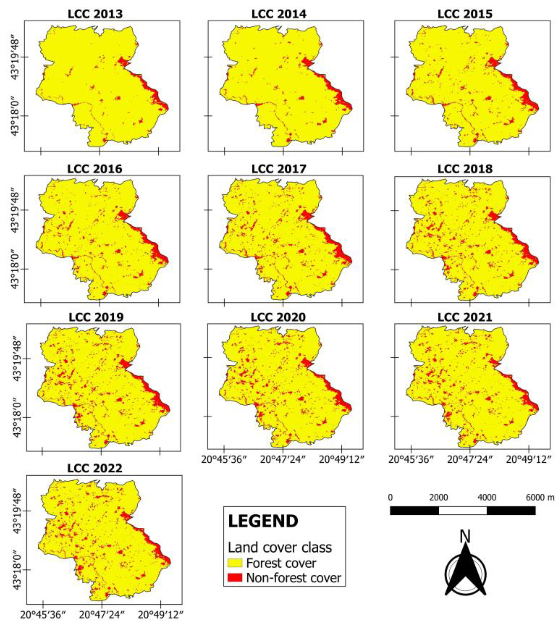
3.1. Forest Cover Loss

Concerning land cover change, the analysis showed (Figure 2) that forest cover loss in the Kopaonik NP rose continuously until the end of the observed period. Until 2017, forest cover loss nearly doubled each year (Figure 3). From 2017 to 2019, forest cover loss increased roughly by 0.5%, and from 2019 to 2020 by 0.14%. The 2021 forest cover loss was identical to that of 2020, while in 2022, forest cover loss increased by 0.28%. In total, 5.75% of forest area was lost on behalf of the non-forest cover (without Norway spruce trees, and not counting the saplings).

In 2014 and 2015, forest cover loss occurred in relatively small areas throughout the analyzed area (

Table 4. Dynamics of cumulative forest cover loss at forest glade (fragment) level.

Year	MEAN (ha)	MIN (ha)	MAX (ha)	SD (ha)
2013	/	/	/	/
2014	0.05	0.02	0.74	0.07
2015	0.07	0.01	0.73	0.10
2016	0.07	0.01	1.60	0.15
2017	0.08	0.01	1.90	0.16
2018	0.12	0.01	3.87	0.28
2019	0.11	0.01	4.60	0.29
2020	0.12	0.01	4.74	0.32
2021	0.14	0.01	5.49	0.35
2022	0.13	0.01	5.72	0.37

and Figure 3). In those years, the maximum area of forest cover loss in terms of fragment level—later referred to as forest glades—did not exceed 1 ha, and this area was quite uniform, as indicated by a low standard deviation. Later, in 2016 and 2017, forest glades emerged in new areas, while existent areas spread out, mainly in the west and northwest, which was particularly evident in 2017 (Figure 3). The mean area of forest glades was almost identical to those from 2014 and 2015, although the maximum area nearly doubled (Table 4). Moreover, the spread of existing forest glades continued in the western and northwestern parts of the research area (

Table 5. Accuracy quantitative measures of LCC.

Year	OA	PA/F	PA/N	UA/F	UA/N
2013	97.9	99.84	69.28	97.97	96.61
2014	97.79	99.56	73.47	98.1	92.41
2015	95.97	99.37	66.14	96.27	92.28
2016	96.78	99.61	72.22	96.9	95.47
2017	92.49	99.17	56.04	92.49	92.49
2018	94.1	99.01	68	95.29	91.27
2019	95.61	99.12	72.28	95.96	92.52
2020	91.83	99.61	55.63	91.26	96.88
2021	92.7	99.41	56.82	92.49	94.76
2022	96.63	99.43	76.3	96.82	94.88

/F—forest cover; /N—non-forest cover.

), which was confirmed by the increased standard deviation. The 2018 results are particularly interesting, as the maximum area of forest glades and standard deviation nearly doubled compared to the previous year (Table 4). The spread of existing forest glades continued in the mentioned areas (Figure 3), while its area increase, as indicated by mean, maximum, and standard deviation values, was the largest in the observed period (Table 4). Interestingly, the results of 2019, 2020, 2021, and 2022 do not significantly differ from 2018 (Table 4), as only a small number of forest glades emerged across the analyzed area, including a small-scale continuous spread of existing glades in the west, northwest, and northeast, which gradually increased until the end of the observed period (Figure 3, Table 4).

Quantitative accuracy assessments showed that the OA was quite high for all years, indicating that the produced maps have the required accuracy (Table 5). However, this should be taken with caution, as the dominance of forest cover pixels (

Table 6. The error matrix populated by estimated proportions of area.

Year	LCC	Forest	Non-Forest	Total (Wi)	Am,i [pixel]	Am,i [ha]
2013	Forest	0.935	0.019	0.954	101,142	2276
	Non-forest	0.002	0.044	0.046	4804	108
	Total	0.937	0.063	1	105,946	2384
2014	Forest	0.928	0.018	0.946	100,211	2255
	Non-forest	0.004	0.050	0.054	5710	128
	Total	0.932	0.068	1	105,921	2383
2015	Forest	0.892	0.034	0.926	220,937	2209
	Non-forest	0.006	0.068	0.074	17,466	175
	Total	0.898	0.102	1	238,403	2384
2016	Forest	0.893	0.029	0.922	219,819	2198
	Non-forest	0.004	0.074	0.078	18,584	186
	Total	0.897	0.103	1	238,403	2384
2017	Forest	0.838	0.068	0.906	216,032	2160
	Non-forest	0.007	0.087	0.094	22,371	224
	Total	0.845	0.155	1	238,403	2384
2018	Forest	0.859	0.042	0.901	214,862	2149
	Non-forest	0.009	0.09	0.099	23,541	235
	Total	0.868	0.132	1	238,403	2384
2019	Forest	0.862	0.035	0.897	214,007	2140
	Non-forest	0.008	0.095	0.103	24,366	244
	Total	0.87	0.130	1	238,373	2384
2020	Forest	0.82	0.079	0.899	214,178	2142
	Non-forest	0.003	0.098	0.101	24,225	242
	Total	0.823	0.177	1	238,403	2384
2021	Forest	0.838	0.068	0.906	215,885	2159
	Non-forest	0.005	0.090	0.095	22,518	225
	Total	0.843	0.157	1	238,403	2384
2022	Forest	0.874	0.029	0.903	215,167	2152
	Non-forest	0.005	0.093	0.098	23,236	232
	Total	0.879	0.122	1	238,403	2384

W_i—mapped area proportions (%), A_m,i—mapped area.

) influences the calculation of the OA. Qualitative accuracy assessment revealed some classification errors in those years, such as misclassification of non-forest cover as forest cover and, rarely, vice-versa. Such errors occurred in areas where individual trees were scattered all across non-forest patches and where the area of the non-forest cover was inconsiderably small (less than 100 m²). It is worth noticing that the PA for non-forest cover was significantly lower than for forest cover (Table 5). Such results indicate that numerous non-forest areas were misclassified as forest cover, especially in the years 2017, 2020, and 2021 (Table 6), which was also pointed out by the qualitative assessment of LCC in those years.

3.2. Evaluation of VI Sensitivity in Detecting Responses to Drought and Predicting the Dieback of Norway Spruce

The results of the VI time series analysis (Figure 4) showed that a large number of VIs used to reflect the Norway spruce response to the severe drought that occurred in 2012, such as the DSWI, NDVI, TCG, TCW, EVI, TVI, and SAVI.

Regardless of drought, the values of other VIs, such as the MSI, NDMI, and NMDI, remained almost constant across all years analyzed. On the other hand, for all VIs used, responses to drought occurring during 2011 were non-existent. As for the post-drought period (2013–2014), the values of VIs regained the pre-drought state.

The analysis showed that the DSWI, NDVI, and TVI in the pre-drought period (2009) did not predict the spatial distribution of forest and non-forest cover (forest cover loss) in 2015 (d < 0.50) (Figure 5). On the other hand, the MSI, NDMI, and NMDI showed a medium effect in predicting the spatial distribution of forest and non-forest cover (forest cover loss) in 2015. As for the EVI, SAVI, TCG, and TCW methods showed a large effect (d≈0.80) in predicting the spatial distribution of forest and non-forest cover (forest cover loss) in 2015.

For the drought period (2011–2012), we also found a large effect for the MSI, NDMI, NMDI, and TCW in predicting forest and non-forest cover (forest cover loss) in 2015, where the strength of such effect slightly increased in 2012 (Figure 5). Moreover, a medium effect in predicting the spatial distribution of forest and non-forest cover (forest cover loss) in 2015 was shown using the DSWI, EVI, SAVI, and TCG in 2011, while, in 2012, only the SAVI and TCG maintained their predicting ability.

The analysis results of the post-drought period (2013–2014) are quite interesting, as contrary to the drought period, the MSI and NDMI now have a medium effect, while the EVI, SAVI, TCG, and TCW have a large effect in predicting the spatial distribution of forest and non-forest cover (forest cover loss) in 2015. The strength of such an effect for the above-mentioned VIs increased to a very large effect (d > 1.20) and reached its peak in 2014. Again, in the same year, the MSI and NDMI showed a large effect in predicting the spatial distribution of forest and non-forest cover (forest cover loss) in 2015.

It is important to note that the NDVI and TVI, through all years analyzed (2009–2014), did not predict the spatial distribution of forest and non-forest cover (forest cover loss) in 2015. Still, the DSWI in 2014 showed a medium effect in predicting the spatial distribution of forest and non-forest cover (forest cover loss) in 2015.

Further analysis showed, in contrast to the previous one, that the NDVI, EVI, SAVI, TVI, and TCG in the pre-drought (2009) and drought (2011–2012) periods did not predict the spatial distribution of forest and non-forest cover (forest cover loss) in 2017 (d < 0.50) (Figure 6). Exceptions were the MSI, NDMI, DSWI, NMDI, and TCW in 2009 and 2011, which showed a medium effect in predicting the spatial distribution of forest and non-forest cover (forest cover loss) in 2017. Starting from 2012 (the year of severe drought), we found a large effect of the MSI, NDMI, NMDI, and TCW (except for DSWI) in predicting the spatial distribution of forest and non-forest cover (forest cover loss) in 2017 (Figure 6). The strength of such a relationship remained constant in 2013, a post-drought year, except for the NMDI, where it slightly increased. In the same year, the NDVI, EVI, SAVI, and TVI, which previously showed no effect in the pre-drought (2009) and drought (2011–2012) periods (d < 0.50), reached a medium effect in predicting the spatial distribution of forest and non-forest cover (forest cover loss) in 2017.

Interestingly, in 2014, another post-drought year, the EVI, SAVI, and TCG showed no effect, while the NDVI and TVI retained a medium effect in predicting the spatial distribution of forest and non-forest cover (forest cover loss) in 2017. It is important to note that the DSWI had a large effect, and the MSI, NMDI, and TCW had a very large effect in predicting the spatial distribution of forest and non-forest cover (forest cover loss) in 2017.

4. Discussion

4.1. Forest Cover Loss

In the example of the Kopaonik NP, it can be seen from the results of this study that Landsat 8 (OLI) and Sentinel 2A/2B (MSI) satellite imagery can be used, with satisfactory accuracy, in the mapping of small forest cover losses. Moreover, the high UA for non-forest cover (Table 5) also indicates satisfactory accuracy, as most pixels classified as non-forest cover represent the real state in the field. Nevertheless, both quantitative and qualitative accuracy assessments showed some minor drawbacks. For example, the lower PA for non-forest cover (Table 5) may indicate the impossibility of correctly classifying areas smaller than 10 × 10 or 15 × 15 m due to spatial resolution limitations of both sensors used (Sentinel 2 MSI up to 10 m and Landsat 8 OLI up to 15 m). Such was the case with KC et al.’s [111] land cover classification of Rupandehi District, Nepal, where barren land was classified as neighboring water bodies due to its small size. Sometimes, in an area of one pixel, we can find many different types of land cover, which significantly alter pixel spectral signature; thus, in the classification process, pixels can be assigned to the wrong land cover class. Inter-seasonal variation in vegetation photosynthetic activity and the current health status of forest cover may also alter its spectral signature, for example, to be similar to the neighboring non-forest cover (grassland or underbrush). This was observed by Forsythe et al. [56] to be the main reason for lower PA values in some classification results. The combination of both events surely contributed to the classification errors. Nevertheless, such errors can be ignored, as the undetected loss of several trees does not represent a significant error from the forestry management point of view.

Considering that 5.75% of the pure Norway spruce forest in the Kopaonik NP ceased to exist in the post-drought period (Figure 2), it is hard to attribute such a state exclusively to the drought effects. Kesić et al. [28] came to the same conclusion, claiming that soil acidification and monodominance of Norway spruce at Mt. Kopaonik were other possible reasons for its dieback. However, the nearly double increase in forest cover loss during 2015 and 2016 (Figure 2) can be easily attributed to the effects of pest outbreaks. As reported by Matović et al. [31] and Stojanović et al. [33], in those years, there was a huge outbreak of I. typographus and P. chalcographus, which, at that moment, acted like a primary pest. However, it should be taken into account that bark beetle outbreaks in Norway spruce forests are a consequence of adverse climatic effects, such as drought, as their defensive mechanisms are weakened when affected by summer drought [112,113,114,115]. Spatial–temporal expansion of forest glades in 2015, 2016, and 2017, which previously emerged over small areas in 2014 (Figure 3 and Table 4), clearly indicate bark beetle activity. Such a trend continued in later years with less intensity, following a decline in bark beetle outbreaks. However, a few questions arise. Is the forest cover loss a result of a single factor or the interaction of several factors? Are particular stands more susceptible to drought than others? The answers to these questions should be sought through the implementation of various long-term multidisciplinary research projects in these forests.

4.2. Evaluation of VI Sensitivity in Detecting Responses to Drought and Predicting the Dieback of Norway Spruce

Although the NDVI, EVI, TVI, SAVI, TCG, DSWI, and TCW revealed a large-scale drop in vegetation vigor and canopy water content all over the analyzed area, that is, the response of Norway spruce to severe drought occurred in 2012 (Figure 4), not all VIs predicted forest cover loss in 2015 (Figure 5). Besides TCW, Cohen’s d showed that other VIs, which did not show any response of Norway spruce to severe drought in 2012 (MSI, NDMI, and NMDI), had large and very large effects in predicting forest cover loss in 2015. A similar result was found for 2011, which was a year with less severe drought occurrence. Although the MSI [46] and NDMI [49] are considered to be highly effective in assessments of moisture stress in plants, this was not the case in our study. Based on such results, we can assume that NIR-SWIR1 ratio-based Water Vis, such as the MSI and NDMI, indicated only different soil water retaining capacities in areas where forest cover loss occurred and where it did not. We found the base for this assumption in a conclusion in Welikhe et al.’s research [104], where it was reported that MSI is strongly correlated to soil moisture at 20 cm depth. On the other hand, in a review study, Le et al. [49] summarized findings from other studies [98,116,117], concluding that the NDWI method (in our research named NDMI) yielded unsatisfactory results when applied to forest objects for water stress monitoring. Worth noticing is the large effect of the pre-drought (2009) results of the EVI, SAVI, TCG, and TCW in predicting the forest cover loss in 2015, as such a state points to pre-drought differences, and possibly the susceptibility of different Norway spruce populations, or their respective habitats, to drought events in the Kopaonik NP. The cause of this may be found in the research of Rehschuh et al. [118], in which they reported that Norway spruce trees growing on shallow, well-drained soil expressed a relatively higher drought sensitivity compared to trees from a site with deep, silty soil. The practically non-existent ability to predict the forest cover loss in 2015, with the post-drought data (2013 and 2014) using the NDVI and its modified version TVI, should not be considered unusual. Although these VIs showed strong sensitivity in the detection of Norway spruce response to severe drought, they cannot be used in predicting forest cover loss, as they do not exhibit any statistically significant difference between VI values in the area of forest and non-forest cover (forest cover loss). As such, we agree with Le et al.’s [49] conclusion stating that the NDVI cannot be effectively used in the early detection of drought effects. On the contrary, other “drought-sensitive” VIs, such as the EVI, SAVI, TCG, and TCW, showed a large (2013) to very large effect (2014) in predicting forest cover loss in 2015, indicating that the post-drought period is crucial in predicting drought effects, as it can strongly suggest where forest cover loss might occur. In contrast, these VIs, except for the TCW, did not perform well in predicting forest cover loss in 2017 (Figure 6), indicating that the primary cause of Norway spruce dieback after 2015 was mainly driven by pest outbreaks. As seen in Figure 2, forest cover loss doubled from 2015 to 2017. Such a finding goes in line with an earlier report from Matović et al. [31], where it was stated that, in those years, bark beetle began to act as a primary pest. What challenges this conclusion is a post-drought medium (2013) to a large effect (2014) of the DSWI and a large (2013) to a very large effect (2014) of the TCW in predicting forest cover loss in 2017 (Figure 6), which may indicate a direct influence of drought on the loss of forest cover in 2017. Nevertheless, so-called Water VIs (MSI, NDMI, and NMDI) performed almost the same as for 2015 forest cover loss prediction—having a large (2012) to very large effect (2013 and 2014) in predicting forest cover loss. Considering these results together with previous conclusions, where we stated that such results only indicated different soil water retaining capacities in areas where forest cover loss occurred and where it did not, we can only confirm such assumptions.

4.3. Implication for Conservation of Norway Spruce Stands in the Kopaonik NP

As indicated by the results, severe drought greatly impacts forest cover loss in Norway spruce stands in the Kopaonik NP. Although severe drought has not occurred since 2012, according to Miletić et al. [37], such events may occur more often in the future. Accordingly, we can only expect that forest cover loss will continue to rise. However, we did not take into account several other reasons, which surely had or may have a great impact on forest cover loss. In their study in the Kopaonik NP, Matović et al. [31] found that devitalization and dieback of Norway spruce trees were more pronounced in structurally and age-homogeneous stands. As such, within areas of protective regimes, it should be legally enabled to implement adequate forest management measures that will support structural and age differentiation. Furthermore, the introduction of complementary species, such as Silver fir (Abies alba Mill.) and European beech (Fagus sylvatica L.), to improve stability and overall resistance of Norway spruce stands should not be neglected, as the monodominance of one species, such as Norway spruce, leads to instability and reduced tolerance to pests and adverse climatic events, as was proven in our and many other studies [119,120,121]. Regarding the deforested areas, support should be provided through tree planting. As Tanovski et al. [116] proposed, this should involve using reproductive material of known origin with adaptive properties suitable for the environmental conditions of the regeneration site.

4.4. Methodological Limitations of the Used Methodology in Detecting Responses to Drought and Predicting the Dieback of Norway Spruce

The main reason for some previously proven VIs, such as the NDWI, MSI, and NDMI [38,116], exhibiting low performance in monitoring and predicting the health status of Norway spruce forests in the Kopaonik NP may be the lower spatial or spectral resolution of the imagery used. Although, from 2015 until 2022, higher spatial and spectral resolution Sentinel 2 (MSI) imagery was used for land cover mapping, strong sensitivity in predicting forest cover loss using lower spatial and spectral resolution Landsat 7 (ETM+) and Landsat 8 (OLI) imagery was simply impossible due to various factors. For example, one pixel in Landsat 7 (ETM+) and Landsat 8 (OLI) imagery may have mixed spectral values, as it, in a spatial manner, contains up to three pixels from Sentinel 2 (MSI) imagery, which may include distinct land cover types. A similar problem was reported in Abdollahnejad et al.’s [42] study, which points out that lower-resolution satellite imagery has limited use; that is, it could be used only in studies where sample sizes are not less than the spatial resolution of used imagery. Taking into account that Sentinel 2 (MSI) has been in orbit since June 23, 2015, such shortcomings, in the context of this study, could not be overcome. Another problem lies in the low temporal resolution and unavailability of cloud-free Landsat 7 (ETM+) and Landsat 8 (OLI) imagery during the entire growing season in Kopaonik NP. If more were available, coupled with ground-measured meteorological data, it would be easier to determine which drought levels or their cumulative effects, along the growing season, trigger Norway spruce dieback in the future. On the other hand, the usage of very-high spatial and spectral resolution imagery, such as Pléiades 1A/1B, QuickBird, SPOT 6/7, WorldView-2, etc., could provide precise and clear answers even at the single tree level. However, their high cost was a limiting factor in the framework of this study. Considering that other factors, such as stand and terrain characteristics, play a significant role in Norway’s spruce dieback [28,31,118], future analyses should include these factors. This can be achieved by employing machine learning methods to provide more accurate and reliable results.

5. Conclusions

Based on the obtained results, remote sensing proved to be a powerful tool in analyzing the spatial–temporal trends of forest cover loss and the sensitivity of VIs in detecting responses to drought and predicting the dieback of Norway spruce in the Kopaonik NP. Our analysis revealed a consistent increase in forest cover loss in the Kopaonik NP until the end of the observed period (2013–2022), which was driven by severe drought in 2011, especially in 2012. Regarding rates of loss, forest cover loss nearly doubled each year, reaching its peak in 2018. Such a state was significantly influenced by emerging bark beetle outbreaks, which acted as a primary pest from 2015 to 2017. Overall, approximately 5.75% of forest cover was lost on behalf of non-forest cover. It was also found that forest cover loss first started in 2014 and 2015, occurring in small areas, but later expanded, particularly in the western and northwestern parts of our study area.

Further analysis revealed that several VIs, including the DSWI, NDVI, EVI, TVI, SAVI, TCG, and TCW, proved to be sensitive in detecting the response of Norway spruce to severe drought in 2012. However, the values of other VIs remained relatively constant across all years, with no observable indication of the response of Norway spruce to drought. The predictive capabilities of VIs for forest cover loss varied across different periods, with some VIs showing a significant effect during drought and post-drought periods (EVI, SAVI, TCG, and TCW). Notably, the NDVI, TVI, and DSWI were unable to predict forest cover loss or exhibited low performance in predicting forest cover loss in 2015 and 2017, respectively. The significant effect of the pre-drought data of the EVI, SAVI, TCG, and TCW in predicting forest cover loss in 2015 indicates that some parts of Norway’s spruce forests are more susceptible to drought than others, possibly due to their differing capacities to retain soil water. Unfortunately, the unavailability of higher spatial and spectral resolution Sentinel 2 (MSI) imagery before 2015 significantly reduced the performance of the used VIs in monitoring and predicting the health status of Norway spruce forests. Nevertheless, the determined sensitivity of VIs to detect the drought-induced response of Norway spruce forests provides valuable insights into the dynamics of forest cover change, with implications for monitoring and conservation efforts in the Kopaonik NP. Accordingly, stakeholders in forestry should seriously consider implementing remote sensing methods within existing forestry management methods for daily use.

References

1. FAO. Forest Extentand Changes. In Global Forest Resources Assessment 2020: Main Report; FAO: Italy, Rome, 2020; pp. 15–19. Available online: https://www.fao.org/3/ca9825en/ca9825en.pdf (accessed on 12 March 2024). [CrossRef]
2. Dudík, R.; Palátová, P.; Jarský, V. Restoration of Declining Spruce Stands in the Czech Republic: A Bioeconomic View on Use of Silver Birch in Case of Small Forest Owners. Austrian J. For. Sci. 2021, 4, 375–394. [Google Scholar]
3. Klavina, D.; Menkis, A.; Gaitnieks, T.; Velmala, S.; Lazdins, A.; Rajala, T.; Pennanen, T. Analysis of Norway spruce dieback phenomenon in Latvia—A belowground perspective. Scand. J. For. Res. 2015, 31, 156–165. [Google Scholar] [CrossRef]
4. Piedallu, C.; Dallery, D.; Bresson, C.; Legay, M.; Gégout, J.; Pierrat, R. Spatial vulnerability assessment of silver fir and Norway spruce dieback driven by climate warming. Landsc. Ecol. 2023, 38, 341–361. [Google Scholar] [CrossRef]
5. Boczoń, A.; Kowalska, A.; Ksepko, M.; Sokołowski, K. Climate Warming and Drought in the Bialowieza Forest from 1950–2015 and Their Impact on the Dieback of Norway Spruce Stands. Water 2018, 10, 1502. [Google Scholar] [CrossRef]
6. Rosner, S.; Luss, S.; Světlík, J.; Andreassen, K.; Børja, I.; Dalsgaard, L.; Evans, R.; Tveito, O.E.; Solberg, S. Chronology of hydraulic vulnerability in trunk wood of conifer trees with and without symptoms of top dieback. J. Plant Hydraul. 2016, 3, e001. [Google Scholar] [CrossRef]
7. Matić, S. The impact of site changes and management methods on dieback of common spruce (Picea abies Karst.) in Croatia. Croat. J. For. Eng. 2011, 32, 7–16. [Google Scholar]
8. Popa, A.; van der Maaten, E.; Popa, I.; van der Maaten-Theunissen, M. Early warning signals indicate climate change-induced stress in Norway spruce in the Eastern Carpathians. Sci. Total Environ. 2024, 912, 169167. [Google Scholar] [CrossRef]
9. Caudullo, G.; Tinner, W.; de Rigo, D. Picea abies in Europe: Distribution, habitat, usage and threats. In European Atlas of Forest Tree Species; San-Miguel-Ayanz, J., de Rigo, D., Caudullo, G., Houston Durrant, T., Mauri, A., Eds.; European Union: Luxembourg, 2016; pp. 114–116. [Google Scholar]
10. Jovanović, B. Picea abies Karst. In Dendrology, 6th ed.; Uskoković, Đ., Ed.; Univerzitetska Štampa: Belgrade, Serbia, 2000; pp. 84–89. [Google Scholar]
11. Banković, S.; Medarević, M.; Pantić, D.; Petrović, N. Forests by Stand Categories, 1st ed.; National Forest Inventory of the Republic of Serbia, Ministry of Agriculture, Tomter, S., Vasiljević, A., Eds.; Forestry and Water Management of the Republic of Serbia, Forest Directorate: Belgrade, Serbia, 2009; pp. 54–55. [Google Scholar]
12. Matović, B. Optimal Condition in Spruce-Fir Forests—Goals and Management Problems at Mountain Zlatar. Master’s Thesis, University of Belgrade, Faculty of Forestry, Belgrade, Serbia, 2005. (In Serbian). [Google Scholar]
13. Kolesnikov, B.P. Forest Vegetation in the South-Eastern Part of the Vychegda Basin; Nauka Publ.: Leningrad, Soviet Union, 1985. [Google Scholar]
14. Eckstein, D.; Krause, C.; Bauch, J. Dendroecological investigations of spruce trees (Picea abies (L.) Karst.) of different damage and canopy classes. Holzforschung 1989, 43, 411–417. [Google Scholar] [CrossRef]
15. Spiecker, H. Growth variation and environmental stresses: Long-term observations on permanent research plots in South-western Germany. Water Air Soil Pollut. 1991, 54, 247–256. [Google Scholar] [CrossRef]
16. Kahle, H.P.; Spiecker, H. Adaptability of radial growth of Norway spruce to climate variations: Results of a site specific dendroecological study in the high elevations of the Black Forest (Germany). Radiocarbon 1996, 9999, 785–801. [Google Scholar]
17. Mäkinen, H.; Nöjd, P.; Kahle, H.P.; Neumann, U.; Tveite, B.; Mielikäinen, K.; Röhle, H.; Spiecker, H. Radial growth variation of Norway spruce (Picea abies (L.) Karst.) across latitudinal and altitudinal gradients in central and northern Europe. Forest Ecol. Manage. 2002, 171, 243–259. [Google Scholar] [CrossRef]
18. Andreassen, K.; Solberg, S.; Tveito, O.E.; Lystad, S.F. Regional differences in climatic responses of Norway spruce (Picea abies (L.) Karst) growth in Norway. Forest Ecol. Manag. 2006, 222, 211–221. [Google Scholar] [CrossRef]
19. Pichler, P.; Oberhuber, W. Radial growth response of coniferous forest trees in an inner Alpine environment to the heat-wave in 2003. Forest Ecol. Manag. 2007, 242, 688–699. [Google Scholar] [CrossRef]
20. Lebourgeois, L. Climatic signal in annual growth variation of silver fir (Abies alba Mill.) and spruce (Picea abies Karst.) from the French Permanent Plot Network (RENECOFOR). Ann. For. Sci. 2007, 64, 333–343. [Google Scholar] [CrossRef]
21. Reichstein, M.; Ciais, P.; Papale, D.; Valentini, R.; Running, S.; Viovy, N.; Cramer, W.; Granier, A.; Ogée, J.; Allard, V.; et al. Reduction of ecosystem productivity and respiration during the European summer 2003 climate anomaly: A joint flux tower, remote sensing and modelling analysis. Glob. Chang. Biol. 2007, 13, 634–651. [Google Scholar] [CrossRef]
22. Van der Maaten-Theunissen, M.; Kahle, H.P.; van der Maaten, E. Drought sensitivity of Norway spruce is higher than that of silver fir along an altitudinal gradient in southwestern Germany. Annal. For. Sci. 2013, 70, 185–193. [Google Scholar] [CrossRef]
23. Pretzsch, H.; Grams, T.; Häberle, K.H.; Pritsch, K.; Bauerle, T.; Rötzer, T. Growth and mortality of Norway spruce and European beech in monospecific and mixed-species stands under natural episodic and experimentally extended drought. Results of the KROOF throughfall exclusion experiment. Trees 2020, 34, 957–970. [Google Scholar] [CrossRef]
24. Begović, K.; Rydval, M.; Mikac, S.; Čupić, S.; Svobodova, K.; Mikoláš, M.; Kozák, D.; Kameniar, O.; Frankovič, M.; Pavlin, J.; et al. Climate-growth relationships of Norway Spruce and silver fir in primary forests of the Croatian Dinaric mountains. Agric. For. Meteorol. 2020, 288–289, 108000. [Google Scholar] [CrossRef]
25. Stangler, D.F.; Miller, T.W.; Honer, H.; Larysch, E.; Puhlmann, H.; Seifert, T.; Kahle, H.-P. Multivariate drought stress response of Norway spruce, silver fir and Douglas fir along elevational gradients in Southwestern Germany. Front. Ecol. Evol. 2022, 10, 907492. [Google Scholar] [CrossRef]
26. D’Andrea, G.; Šimunek, V.; Pericolo, O.; Vacek, Z.; Vacek, S.; Corleto, R.; Olejár, L.; Ripullone, F. Growth Response of Norway Spruce (Picea abies [L.] Karst.) in Central Bohemia (Czech Republic) to Climate Change. Forests 2023, 14, 1215. [Google Scholar] [CrossRef]
27. Bouriaud, O.; Popa, I. Comparative dendroclimatic study of Scots pine, Norway spruce, and silver fir in the Vrancea Range, Eastern Carpathian. Trees 2009, 23, 95–106. [Google Scholar] [CrossRef]
28. Kesić, L.; Matović, B.; Stojnić, S.; Stjepanović, S.; Stojanović, D. Climate Change as a Factor Reducing the Growth of Trees in the Pure Norway Spruce Stand (Picea abies (L.) H. Karst.) in the National Park “Kopaonik”. Topola/Poplar 2016, 197–198, 25–34. [Google Scholar]
29. Levanič, T.; Gričar, J.; Gagen, M.; Jalkanen, R.; Loader, N.J.; McCarroll, D.; Oven, P.; Robertson, I. The climate sensitivity of Norway spruce [Picea abies (L.) Karst.] in the southeastern European Alps. Trees 2009, 23, 169–180. [Google Scholar] [CrossRef]
30. Karadžić, D.; Milanović, S.; Golubović Ćurguz, V. Climatic conditions that preceded the massive dieback of Norway spruce stands at Mt. Golija. In Causes of Spruce (Picea abies Karst.) Dieback in the Area of the Nature Park “Golija”; University of Belgrade, Faculty of Forestry: Belgrade, Serbia, 2017; pp. 15–17. (In Serbian) [Google Scholar]
31. Matović, B.; Stojanović, D.; Kesić, L.; Stjepanović, S. Impact of Climate on Growth and Vitality of Norway Spruce at Kopaonik Mountain. Topola/Poplar 2018, 201–202, 99–116. (In Serbian) [Google Scholar]
32. Vemić, A.; Milenković, I. Contribution to the Knowledge of Top Dying of Norway Spruce in The Forests of Serbia and Montenegro. Forestry/Šumarstvo 2021, 1–2, 189–199. [Google Scholar]
33. Stojanović, B.D.; Orlović, S.; Zlatković, M.; Kostić, S.; Vasić, V.; Miletić, B.; Kesić, L.; Matović, B.; Božanić, D.; Pavlović, L.; et al. Climate change within Serbian forests: Current state and future perspectives. Topola/Poplar 2021, 208, 39–56. [Google Scholar] [CrossRef]
34. Zahirović, K.; Dautbašić, M.; Mujezinović, O. Dieback of Spruce Stands Caused by Bark Beetles in Central Bosnia. Our Forests/Naše Šume 2014, 36–37, 4–13. [Google Scholar]
35. Dautbašić, M.; Bjelić, M.; Mujezinović, O. Forest Decline in the Area on Zenica—Doboj Canton. Our Forests/Naše šume 2014, 38–39, 5–15. [Google Scholar]
36. Ballian, D.; Božić, G. Biochemical Variability of Spruce (Picea abies Karst) in Bosnia and Herzegovina; UŠIT FBiH: Sarajevo, Bosnia and Herzegovina; Silva Slovenica: Ljubljana, Slovenia, 2018; p. 14. [Google Scholar]
37. Miletić, B.; Orlović, S.; Lalić, B.; Đurđević, V.; Vujadinović Mandić, M.; Vuković, A.; Gutalj, M.; Stjepanović, S.; Matović, B.; Stojanović, D.B. The potential impact of climate change on the distribution of key tree species in Serbia under RCP 4.5 and RCP 8.5 scenarios. Austrian J. For. Sci. 2021, 138, 183–208. [Google Scholar]
38. Assal, T.J.; Anderson, P.J.; Sibold, J. Spatial and temporal trends of drought effects in a heterogeneous semi-arid forest ecosystem. For. Ecol. Manag. 2016, 365, 137–151. [Google Scholar] [CrossRef]
39. Hais, M.; Neudertová Hellebrandová, K.; Šrámek, V. Potential of Landsat spectral indices in regard to the detection of forest health changes due to drought effects. J. For. Sci. 2018, 65, 70–78. [Google Scholar] [CrossRef]
40. Páscoa, P.; Gouveia, C.M.; Russo, A.C.; Bojariu, R.; Vicente-Serrano, S.M.; Trigo, R.M. Drought Impacts on Vegetation in Southeastern Europe. Remote Sens. 2020, 12, 2156. [Google Scholar] [CrossRef]
41. Avetisyan, D.; Borisova, D.; Velizarova, E. Integrated Evaluation of Vegetation Drought Stress through Satellite Remote Sensing. Forests 2021, 12, 974. [Google Scholar] [CrossRef]
42. Abdollahnejad, A.; Panagiotidis, D.; Surový, P.; Modlinger, R. Investigating the Correlation between Multisource Remote Sensing Data for Predicting Potential Spread of Ips typographus L. Spots in Healthy Trees. Remote Sens. 2021, 13, 4953. [Google Scholar] [CrossRef]
43. DeRose, R.J.; Long, J.N.; Ramsey, R.D. Combining dendrochronological data and the disturbance index to assess Engelmann spruce mortality caused by a spruce beetle outbreak in southern Utah, USA. Remote Sens. Environ. 2011, 115, 2342–2349. [Google Scholar] [CrossRef]
44. Lausch, A.; Heurich, M.; Gordalla, D.; Dobner, H.-J.; Gwillym-Margianto, S.; Salbach, C. Forecasting potential bark beetle outbreaks based on spruce forest vitality using hyperspectral remote-sensing techniques at different scales. For. Ecol. Manag. 2013, 308, 76–89. [Google Scholar] [CrossRef]
45. Havašová, M.; Bucha, T.; Ferenčík, J.; Jakuš, R. Applicability of a vegetation indices-based method to map bark beetle outbreaks in the High Tatra Mountains. Ann. For. Res. 2015, 58, 295–310. [Google Scholar] [CrossRef]
46. Stych, P.; Lastovicka, J.; Hladky, R.; Paluba, D. Evaluation of the Influence of Disturbances on Forest Vegetation Using the Time Series of Landsat Data: A Comparison Study of the Low Tatras and Sumava National Parks. ISPRS Int. J. Geo-Inf. 2019, 8, 71. [Google Scholar] [CrossRef]
47. Dalponte, M.; Solano-Correa, Y.T.; Frizzera, L.; Gianelle, D. Mapping a European Spruce Bark Beetle Outbreak Using Sentinel-2 Remote Sensing Data. Remote Sens. 2022, 14, 3135. [Google Scholar] [CrossRef]
48. Mandl, L.; Lang, S. Uncovering Early Traces of Bark Beetle Induced Forest Stress via Semantically Enriched Sentinel-2 Data and Spectral Indices. PFG 2023, 91, 211–231. [Google Scholar] [CrossRef]
49. Le, T.S.; Harper, R.; Dell, B. Application of Remote Sensing in Detecting and Monitoring Water Stress in Forests. Remote Sens. 2023, 15, 3360. [Google Scholar] [CrossRef]
50. Bright, B.C.; Hudak, A.T.; Meddens, A.J.H.; Egan, J.M.; Jorgensen, C.L. Mapping Multiple Insect Outbreaks across Large Regions Annually Using Landsat Time Series Data. Remote Sens. 2020, 12, 1655. [Google Scholar] [CrossRef]
51. Candotti, A.; De Giglio, M.; Dubbini, M.; Tomelleri, E. A Sentinel-2 Based Multi-Temporal Monitoring Framework for Wind and Bark Beetle Detection and Damage Mapping. Remote Sens. 2022, 14, 6105. [Google Scholar] [CrossRef]
52. Fernandez-Carrillo, A.; Patočka, Z.; Dobrovolný, L.; Franco-Nieto, A.; Revilla-Romero, B. Monitoring Bark Beetle Forest Damage in Central Europe. A Remote Sensing Approach Validated with Field Data. Remote Sens. 2020, 12, 3634. [Google Scholar] [CrossRef]
53. Basak, D.; Bose, A.; Roy, S.; Chowdhury, I.R. Chapter 17—Understanding the forest cover dynamics and its health status using GIS-based analytical hierarchy process: A study from Alipurduar district, West Bengal, India. In Water, Land, and Forest Susceptibility and Sustainability; Chatterjee, U., Pradhan, B., Kumar, S., Saha, S., Zakwan, M., Fath, B.D., Fiscus, D., Eds.; Elsevier Inc.: Amsterdam, The Netherlands, 2023; Volume 1, pp. 475–508. [Google Scholar] [CrossRef]
54. Bochenek, Z.; Ziolkowski, D.; Bartold, M.; Orlowska, K.; Ochtyra, A. Monitoring forest biodiversity and the impact of climate on forest environment using high-resolution satellite images. Eur. J. Remote Sens. 2017, 51, 166–181. [Google Scholar] [CrossRef]
55. Meng, J.; Li, S.; Wang, W.; Liu, Q.; Xie, S.; Ma, W. Mapping Forest Health Using Spectral and Textural Information Extracted from SPOT-5 Satellite Images. Remote Sens. 2016, 8, 719. [Google Scholar] [CrossRef]
56. Forsythe, K.; McCartney, G. Investigating Forest Disturbance Using Landsat Data in the Nagagamisis Central Plateau, Ontario, Canada. ISPRS Int. J. Geo-Inf. 2014, 3, 254–273. [Google Scholar] [CrossRef]
57. Jovanović, D.; Govedarica, M.; Đorđević, I.; Pajić, V. Object based image analysis in forestry change detection. In Proceedings of the IEEE 8th International Symposium on Intelligent Systems and Informatics, Subotica, Serbia, 10–11 September 2010; pp. 231–236. [Google Scholar] [CrossRef]
58. Jovanović, D.; Govedarica, M.; Sabo, F.; Bugarinović, Ž.; Novović, O.; Beker, T.; Lauter, M. Land cover change detection by using remote sensing: A case study of Zlatibor (Serbia). Geogr. Pannonica 2015, 19, 162–173. [Google Scholar] [CrossRef]
59. Valjarević, A.; Djekić, T.; Stevanović, V.; Ivanović, R.; Jandziković, B. GIS numerical and remote sensing analyses of forest changes in the Toplica region for the period of 1953–2013. Appl. Geogr. 2018, 92, 131–139. [Google Scholar] [CrossRef]
60. Milanović, M.M.; Micić, T.; Lukić, T.; Nenadović, S.S.; Basarin, B.; Filipović, D.J.; Tomić, M.; Samardžić, I.; Srdić, Z.; Nikolić, G.; et al. Application of Landsat-Derived NDVI in Monitoring and Assessment of Vegetation Cover Changes in Central Serbia. Carpathian J. Earth Environ. Sci. 2018, 14, 119–129. [Google Scholar] [CrossRef]
61. Kovačević, J.; Cvijetinović, Ž.; Lakušić, D.; Kuzmanović, N.; Šinžar-Sekulić, J.; Mitrović, M.; Stančić, N.; Brodić, N.; Mihajlović, D. Spatio-Temporal Classification Framework for Mapping Woody Vegetation from Multi-Temporal Sentinel-2 Imagery. Remote Sens. 2020, 12, 2845. [Google Scholar] [CrossRef]
62. Jovanović, D.; Gavrilović, M.; Borisov, M.; Govedarica, M. Deforestation Monitoring with Sentinel 1 and Sentinel 2 Images—The Case Study of Fruska Gora (Serbia). Šumarski List. 2021, 3–4, 127–135. [Google Scholar] [CrossRef]
63. Potić, I.; Srdić, Z.; Vakanjac, B.; Bakrač, S.; Ðordević, D.; Banković, R.; Jovanović, J.M. Improving Forest Detection Using Machine Learning and Remote Sensing: A Case Study in Southeastern Serbia. Appl. Sci. 2023, 13, 8289. [Google Scholar] [CrossRef]
64. Jovanović, M.M.; Milanović, M.M. Remote Sensing and Forest Conservation: Challenges of Illegal Logging in Kursumlija Municipality (Serbia). In Forest Ecology and Conservation; Chakravarty, S., Shukla, G., Eds.; IntechOpen: Rijeka, Croatia, 2017; pp. 99–118. [Google Scholar] [CrossRef]
65. Jovanović, M.M.; Milanović, M.M.; Vračarević, R.B. Chapter 1—Comparing NDVI and Corine Land Cover as Tools for Improving National Forest Inventory Updates and Preventing Illegal Logging in Serbia. In Vegetation; Sebata, A., Ed.; IntechOpen: London, UK, 2017; pp. 1–22. [Google Scholar] [CrossRef]
66. Potić, I.; Ćurčić, N.; Potić, M.; Radovanović, M.; Tretiakova, T. Remote sensing role in environmental stress analysis: East Serbia wildfires case study (2007–2017). J. Geogr. Inst. “Jovan Cvijić” SASA 2017, 67, 249–264. [Google Scholar] [CrossRef]
67. Brovkina, O.; Stojanović, M.; Milanović, S.; Latypov, I.; Marković, N.; Cienciala, E. Monitoring of post-fire forest scars in Serbia based on satellite Sentinel-2 data. Geomat. Nat. Hazards Risk 2020, 11, 2315–2339. [Google Scholar] [CrossRef]
68. Jovanović, M.M.; Milanović, M.M. Normalized Difference Vegetation Index (NDVI) as the Basis for Local Forest Management. Example of the Municipality of Topola, Serbia. Pol. J. Environ. Stud. 2015, 24, 529–535. [Google Scholar]
69. Nonić, D.; Šumarac, P.; Ranković, N.; Đorđević, I.; Nedeljković, J. Sustainable Management of the National Park Kopaonik—Opportunities and Challenges; Special edition; Bulletin of the Faculty of Forestry, University of Belgrade: Belgrade, Serbia, 2023; pp. 59–80, (In Serbian). [Google Scholar] [CrossRef]
70. Horwath Consulting Zagreb (HCS). Master Plan for the Kopaonik Tourist Destination (Final Report); Ordering Party: Ministry of Economy and Regional Development of the Republic of Serbia: Belgrade, Serbia, 2009; pp. 14–20. (In Serbian) [Google Scholar]
71. Đorđević, N.; Lakićević, N.; Milićević, S. Benchmarking analysis of tourism in national parks Tara and Kopaonik. Ekon. Teor. I Praksa 2018, 3, 52–70. (In Serbian) [Google Scholar] [CrossRef]
72. Ostojić, D.; Krsteski, B.; Dinić, A.; Perković, A. Vegetation Characteristics of Forest Ecosystems on “Kopaonik” National Park with the Reference to the Forests with the Protection Regime Level I. Šumarstvo/Forestry 2018, 3–4, 179–194. (In Serbian) [Google Scholar]
73. MEP (Ministry of Environmental Protection); PE (Public Enterprise) National Park ‘’Kopaonik”. National Park Kopaonik Management Program for 2021, p. 12. 2020. Available online: https://npkopaonik.rs/wp-content/uploads/2021/08/Program-upravljanja-2021..pdf (accessed on 15 January 2024). (In Serbian).
74. Republic Hydrometeorological Service of the Republic of Serbia (RHMS). Climatology: 30 Years Averages (1991–2020). 2024. Available online: https://www.hidmet.gov.rs/latin/meteorologija/klimatologija_srednjaci.php (accessed on 13 March 2024). (In Serbian)
75. Republic Hydrometeorological Service of the Republic of Serbia (RHMS). Climatology: 30 Years Averages (1961–1990). 2024. Available online: http://www.hidmet.gov.rs/eng/meteorologija/klimatologija_srednjaci.php (accessed on 13 March 2024).
76. Congedo, L. Semi-Automatic Classification Plugin: A Python tool for the download and processing of remote sensing images in QGIS. J. Open Source Softw. 2021, 6, 3172. [Google Scholar] [CrossRef]
77. Chavez, P.S. Image-Based Atmospheric Corrections—Revisited and Improved Photogrammetric Engineering and Remote Sensing, [Falls Church, Va.]. Am. Soc. Photogramm. 1996, 62, 1025–1036. [Google Scholar]
78. Roy, D.P.; Kovalskyy, V.; Zhang, H.K.; Vermote, E.F.; Yan, L.; Kumar, S.S.; Egorov, A. Characterization of Landsat-7 to Landsat-8 reflective wavelength and normalized difference vegetation index continuity. Remote Sens. Environ. 2016, 185, 57–70. [Google Scholar] [CrossRef] [PubMed]
79. Johnson, B.; Tateishi, R.; Hoan, N. Satellite Image Pansharpening Using a Hybrid Approach for Object-Based Image Analysis. ISPRS Int. J. Geo-Inf. 2012, 1, 228–241. [Google Scholar] [CrossRef]
80. Rahaman, K.; Hassan, Q.; Ahmed, M. Pan-Sharpening of Landsat-8 Images and Its Application in Calculating Vegetation Greenness and Canopy Water Contents. ISPRS Int. J. Geo-Inf. 2017, 6, 168. [Google Scholar] [CrossRef]
81. R Core Team. R: A Language and Environment for Statistical Computing; R Foundation for Statistical Computing: Vienna, Austria, 2023; Available online: https://www.R-project.org/ (accessed on 2 November 2023).
82. Hijmans, R.; Raster: Geographic Data Analysis and Modeling. R Package Version 3.6-26. 2023. Available online: https://CRAN.R-project.org/package=raster (accessed on 8 January 2024).
83. Richards, A.J.; Jia, X. Remote Sensing Digital Image Analysis, 4th ed.; Springer: Berlin/Heidelberg, Germany, 2006. [Google Scholar] [CrossRef]
84. Nagamani, K.; Jayakumar, K.; Suresh, Y.; Sriganesh, J. Study on Error Matrix Analysis of Classified Remote Sensed Data for Pondicherry Coast. J. Adv. Res. GeoSci. Rem. Sens. 2015, 2, 3–4. [Google Scholar]
85. Cochran, W.G. Sampling Techniques, 3rd ed.; John Wiley & Sons: New York, NY, USA, 1977. [Google Scholar]
86. Olofsson, P.; Foody, G.M.; Stehman, S.V.; Woodcock, C.E. Making better use of accuracy data in land change studies: Estimating accuracy and area and quantifying uncertaintyusing stratified estimation. Remote Sens. Environ. 2013, 129, 122–131. [Google Scholar] [CrossRef]
87. Pebesma, E.; Bivand, R. Introduction to sf and stars. In Spatial Data Science: With Applications in R, 1st ed.; Chapman and Hall/CRC: Boca Raton, FL, USA, 2023. [Google Scholar] [CrossRef]
88. Neuwirth, E.; RColorBrewer: ColorBrewer Palettes. R Package Version 1.1-3. 2022. Available online: https://CRAN.R-project.org/package=RColorBrewer (accessed on 8 January 2024).
89. Wickham, H. ggplot2: Elegant Graphics for Data Analysis; Springer: New York, NY, USA, 2016; Available online: https://ggplot2.tidyverse.org (accessed on 8 January 2024).
90. Aphalo, P.; ggpmisc: Miscellaneous Extensions to ‘ggplot2’. R Package Version 0.5.5. 2023. Available online: https://CRAN.R-project.org/package=ggpmisc (accessed on 8 January 2024).
91. Pedersen, T.; patchwork: The Composer of Plots. R Package Version 1.2.0. 2024. Available online: https://CRAN.R-project.org/package=patchwork (accessed on 8 January 2024).
92. Iannone, R.; Cheng, J.; Schloerke, B.; Hughes, E.; Lauer, A.; Seo, J.; gt: Easily Create Presentation-Ready Display Tables. R Package Version 0.10. 2023. Available online: https://CRAN.R-project.org/package=gt (accessed on 8 January 2024).
93. Pettorelli, N.; Vik, J.O.; Mysterud, A.; Gaillard, J.M.; Tucker, C.J.; Stenseth, N.C. Using the satellite-derived NDVI to assess ecological responses to environmental change. Trends Ecol. Evol. 2005, 20, 503–510. [Google Scholar] [CrossRef] [PubMed]
94. Huete, A.; Didan, K.; Miura, T.; Rodriguez, E.P.; Gao, X.; Ferreira, L.G. Overview of the radiometric and biophysical performance of the MODIS vegetation indices. Remote Sens. Environ. 2002, 83, 195–213. [Google Scholar] [CrossRef]
95. Tuominen, J.; Lipping, T.; Kuosmanen, V.; Haapane, R. Remote Sensing of Forest Health. In Geoscience and Remote Sensing, 1st ed.; Ho, P., Ed.; InTech: London, UK, 2009; pp. 29–52. [Google Scholar] [CrossRef]
96. Lambert, J.; Drenou, C.; Denux, J.-P.; Balent, G.; Cheret, V. Monitoring forest decline through remote sensing time series analysis. GIScience Remote Sens. 2013, 50, 437–457. [Google Scholar] [CrossRef]
97. Wang, L.; Luo, Y.Q.; Huang, H.G.; Shi, J.; Keliövaara, K.; Teng, W.X.; Qi, G.X. Reflectance features of water stressed Larix gmelinii needles. For. Stud. China 2009, 11, 28–33. [Google Scholar] [CrossRef]
98. Wang, L.; Qu, J.J. NMDI: A normalized multi-band drought index for monitoring soil and vegetation moisture with satellite remote sensing. Geophys. Res. Lett. 2007, 34, L20405. [Google Scholar] [CrossRef]
99. Baig, M.H.A.; Zhang, L.; Shuai, T.; Tong, Q. Derivation of a tasselled cap transformation based on Landsat 8 at-satellite reflectance. Remote Sens. Lett. 2014, 5, 423–431. [Google Scholar] [CrossRef]
100. Lastovicka, J.; Svec, P.; Paluba, D.; Kobliuk, N.; Svoboda, J.; Hladky, R.; Stych, P. Sentinel-2 Data in an Evaluation of the Impact of the Disturbances on Forest Vegetation. Remote Sens. 2020, 12, 1914. [Google Scholar] [CrossRef]
101. Healey, S.; Cohen, W.; Zhiqiang, Y.; Krankina, O. Comparison of Tasseled Cap-based Landsat data structures for use in forest disturbance detection. Remote Sens. Environ. 2005, 97, 301–310. [Google Scholar] [CrossRef]
102. Wickham, H.; Bryan, J.; readxl: Read Excel Files. R Package Version 1.4.3. 2023. Available online: https://CRAN.R-project.org/package=readxl (accessed on 8 January 2024).
103. Welikhe, P.; Quansah, J.E.; Fall, S.; McElhenney, W. Estimation of Soil Moisture Percentage Using LANDSAT-based Moisture Stress Index. J. Remote Sens. GIS 2017, 6, 1–5. [Google Scholar] [CrossRef]
104. Jiang, Z.; Huete, A.R.; Chen, J.; Chen, Y.; Li, J.; Yan, G.; Zhang, X. Analysis of NDVI and scaled difference vegetation index retrievals of vegetation fraction. Remote Sens. Environ. 2006, 101, 366–378. [Google Scholar] [CrossRef]
105. Fraga, H.; Amraoui, M.; Malheiro, A.C.; Moutinho-Pereira, J.; Eiras-Dias, J.; Silvestre, J.; Santos, J.A. Examining the relationship between the Enhanced Vegetation Index and grapevine phenology. Eur. J. Remote Sens. 2014, 47, 753–771. [Google Scholar] [CrossRef]
106. Mancino, G.; Ferrara, A.; Padula, A.; Nolè, A. Cross-Comparison between Landsat 8 (OLI) and Landsat 7 (ETM+) Derived Vegetation Indices in a Mediterranean Environment. Remote Sens. 2020, 12, 291. [Google Scholar] [CrossRef]
107. Cohen, J. The t Test for Means. In Statistical Power Analysis for the Behavioral Sciences, 2nd ed.; Lawrence Erlbaum Associates: Hillsdale, NJ, USA, 1988; pp. 19–27. [Google Scholar]
108. Navarro, D.J. Learning Statistics with R: A Tutorial for Psychology Students and Other Beginners; Version 0.6; University of New South Wales: Sydney, Australia, 2015; Available online: https://learningstatisticswithr.com (accessed on 8 January 2024).
109. Sawilowsky, S. New effect size rules of thumb. J. Mod. Appl. Stat. Methods 2009, 8, 467–474. [Google Scholar] [CrossRef]
110. KC, A.; Wagle, N.; Acharya, T.D. Spatiotemporal Analysis of Land Cover and the Effects on Ecosystem Service Values in Rupandehi, Nepal from 2005 to 2020. ISPRS Int. J. Geo-Inf. 2021, 10, 635. [Google Scholar] [CrossRef]
111. Marini, L.; Økland, B.; Jönsson, A.M.; Bentz, B.; Carroll, A.; Forster, B.; Grégoire, J.C.; Hurling, R.; Nageleisen, L.M.; Netherer, S.; et al. Climate drivers of bark beetle outbreak dynamics in Norway spruce forests. Ecography 2017, 40, 1426–1435. [Google Scholar] [CrossRef]
112. Hlásny, T.; Zimová, S.; Merganičová, K.; Štěpánek, P.; Modlinger, R.; Turčáni, M. Devastating outbreak of bark beetles in the Czech Republic: Drivers, impacts, and management implications. For. Ecol. Manag. 2021, 490, 119075. [Google Scholar] [CrossRef]
113. Seidl, R.; Müller, J.; Hothorn, T.; Bässler, C.; Heurich, M.; Kautz, M. Small beetle, large-scale drivers: How regional and landscape factors affect outbreaks of the European spruce bark beetle. J. Appl. Ecol. 2015, 53, 530–540. [Google Scholar] [CrossRef] [PubMed]
114. Netherer, S.; Lehmanski, L.; Bachlehner, A.; Rosner, S.; Savi, T.; Schmidt, A.; Huang, J.; Paiva, M.R.; Mateus, E.; Hartmann, H.; et al. Drought increases Norway spruce susceptibility to the Eurasian spruce bark beetle and its associated fungi. New Phytol. 2024, 1–18. [Google Scholar] [CrossRef] [PubMed]
115. Moreno, A.; Maselli, F.; Chiesi, M.; Genesio, L.; Vaccari, F.; Seufert, G.; Gilabert, M.A. Monitoring water stress in Mediterranean semi-natural vegetation with satellite and meteorological data. Int. J. Appl. Earth Obs. Geoinf. 2014, 26, 246–255. [Google Scholar] [CrossRef]
116. Dotzler, S.; Hill, J.; Buddenbaum, H.; Stoffels, J. The Potential of EnMAP and Sentinel-2 Data for Detecting Drought Stress Phenomena in Deciduous Forest Communities. Remote Sens. 2015, 7, 14227–14258. [Google Scholar] [CrossRef]
117. Rehschuh, R.; Mette, T.; Menzel, A.; Buras, A. Soil properties affect the drought susceptibility of Norway spruce. Dendrochronologia 2017, 45, 81–89. [Google Scholar] [CrossRef]
118. Kiseleva, V.; Korotkov, S.; Stonozhenko, L.; Naidenova, E. Structure and regeneration of spruce forests as affected by forest management practices in the Moscow Region. IOP Conf. Ser. Earth Environ. Sci. 2019, 226, 012042. [Google Scholar] [CrossRef]
119. Chernenkova, T.; Kotlov, I.; Belyaeva, N.; Suslova, E.; Morozova, O.; Pesterova, O.; Arkhipova, M. Role of Silviculture in the Formation of Norway Spruce Forests along the Southern Edge of Their Range in the Central Russian Plain. Forests 2020, 11, 778. [Google Scholar] [CrossRef]
120. Neuner, S.; Albrecht, A.; Cullmann, D.; Engels, F.; Griess, V.C.; Hahn, W.A.; Hanewinkel, M.; Härtl, F.; Kölling, C.; Staupendahl, K.; et al. Survival of Norway spruce remains higher in mixed stands under a dryer and warmer climate. Glob. Change Biol. 2014, 21, 935–946. [Google Scholar] [CrossRef] [PubMed]
121. Tanovski, V.; Matović, B.; Kesić, L.; Stojanović, D.B. A review of the influence of climate change on coniferous forests in the Balkan peninsula. Topola/Poplar 2022, 210, 41–64. [Google Scholar] [CrossRef]
Figure 1. Study area (location of the Kopaonik NP).
Forests 15 00662 g001
Figure 2. Annual forest cover loss after drought in the Kopaonik NP.
Forests 15 00662 g002
Figure 3. Change in forest cover over ten years (2013–2022).
Forests 15 00662 g003
Figure 4. Time series showing differences in mean values of VIs for forest and non-forest cover (forest cover loss) taken from 2015 (left) and 2017 (right) LCC.
Forests 15 00662 g004
Figure 5. Evaluation of VI sensitivity in predicting forest cover loss in 2015 (gray—no effect, green to red gradient color scale–medium to very large effect).
Forests 15 00662 g005
Figure 6. Evaluation of VI sensitivity in predicting forest cover loss in 2017 (gray—no effect, green to red gradient color scale–medium to very large effect).
Forests 15 00662 g006