Article

Driving Factors and Spatial Distribution of Aboveground Biomass in the Managed Forest in the Terai Region of Nepal

1
School of Forestry, Beijing Forestry University, Haidian District, Beijing 100107, China
2
Institute of Forestry, Tribhuvan University, Hetauda 44107, Nepal
3
College of Forestry, Agricultural and Natural Resources, University of Arkanas at Monticello, Monticello, AR 71656, USA
4
Department of Geosciences and Geography, University of Helsinki, P.O. Box 64, FI-00014 Helsinki, Finland
5
Forest Nepal, Amar Marg 88, C3534, Butwal 32907, Nepal
*
Authors to whom correspondence should be addressed.
Forests 2024, 15(4), 663; https://doi.org/10.3390/f15040663
Submission received: 6 March 2024 / Revised: 27 March 2024 / Accepted: 3 April 2024 / Published: 5 April 2024
(This article belongs to the Special Issue Modeling Aboveground Forest Biomass: New Developments)

Abstract

:
Above-ground biomass (AGB) is affected by numerous factors, including topography, climate, land use, or tree/forest attributes. Investigating the distribution and driving factors of AGB within the managed forests in Nepal is crucial for developing effective strategies for climate change mitigation, and sustainable forest management and conservation. A total of 110 field plots (circular 0.02 ha plots with a 9 m radius), and airborne laser scanning (ALS)-light detection and ranging (LiDAR) data were collected in 2021. The random forest (RF) model was employed to predict the AGB at a 30 m × 30 m resolution based on 32 LiDAR metrics derived from ALS returns. The study assessed the relationships between the AGB distribution and nine independent variables using statistical techniques like the random forest model and partial dependence plots. Results showed that the mean value of the estimated AGB was 120 tons/ha, ranging from 0 to 446.42 tons/ha. AGB showed higher values in the northeast and southeast regions, gradually decreasing towards the northwest. Land use land cover, mean annual temperature, and mean annual precipitation were identified as the primary factors influencing the variability in AGB distribution, accounting for 64% of the variability. Elevation, slope, and distance from rivers were positively correlated with AGB, while proximity to roads had a negative correlation. The increase in precipitation and temperature contributed to the initial rise in AGB, but beyond a certain lag, these variables led to a decline in AGB. This study showed the efficiency of the random forest model and partial dependence plots in examining the relationship between the AGB and its driving factors within managed forests. The study highlights the importance of understanding the AGB driving factors and utilizing LiDAR data for informed decisions regarding the region’s sustainable forest management and climate change mitigation efforts.

1. Introduction

Forests play a crucial role in absorbing atmospheric carbon dioxide, acting as a reservoir that helps counterbalance human-caused greenhouse gas emissions to mitigate climate change impacts [1,2,3]. Carbon storage in forests represents the largest portion, accounting for 82.5% of the total carbon stored in terrestrial vegetation. This significant carbon reservoir plays a vital role in acting as the primary component of the vegetation carbon sink [4,5]. Tropical forests store about 55% of the total carbon in forests and contribute to 70% of the global forest carbon sink [3,6]. Deforestation and forest degradation can lead to carbon emissions entering the atmosphere, affecting global climate and environmental change [7,8,9,10]. Despite the critical role of forests in mitigating climate change through carbon sequestration, there is a significant challenge in accurately estimating the forest biomass and understanding the factors influencing its dynamics. The current concerns about global change and the functioning of ecosystems require accurate forest biomass estimates and an examination of its dynamics [11].
In terrestrial forest ecosystems, the above-ground biomass (AGB) of trees serves as the most crucial and prominent carbon reserve [12,13]. Though field measurements offer precise data on AGB estimation, the sampling process can be constrained by challenging terrain or limited resources. In recent years, remote sensing (RS) technology has emerged as the most preferred method, enabling researchers to obtain a broad-scale, real-time overview of vegetation conditions. This advancement has provided a valuable tool for studying and monitoring vegetation on a large scale [14,15]. Integrating remote sensing data with forest inventory data has evolved into a potent technique for accurately estimating AGB in forest stands [16,17]. Based on remote sensors’ information and allometric equations, the predicted AGB has been calibrated and validated with ground truth to develop biomass estimation models [18]. Remote sensing data, such as light detection and ranging (LiDAR) data, proves advantageous in assessing forest characteristics like tree height, which directly correlates with forest biomass [17,19]. Over the past few years, airborne laser scanning (ALS), alternatively referred to as light detection and ranging (LiDAR), has emerged as the prevailing technology for acquiring precise topographic information, and it has been extensively applied in vegetation mapping and forest inventory, respectively [17,20,21]. ALS data captures the horizontal and vertical distribution of the forest canopies and does not saturate the spectral response of dense canopies, in contrast to multispectral imagery or aerial photography [22]. This advancement of RS technology, integrated with intensive site-based inventory methods, has also played a crucial role in monitoring and managing forests, particularly in initiatives like REDD+ (reducing emissions from deforestation and forest degradation) [23].
In tropical and subtropical forests, carbon stocks are declining at a rate of 1–2 billion tons per year [24] and are primarily affected by different drivers, such as the forest management regime and natural disturbance [25,26,27,28], the species composition of forests and forest type [29], and stand age structure [30,31]. The accumulation of AGB and its distribution in forested ecosystems are also significantly influenced by climate [32,33], as well as soil characteristics and topography [34,35]. Climatic data plays a significant role in understanding how temperature and precipitation influence tree growth [36], resulting in variation in AGB accumulation [37]. Moreover, the variation in AGB of forest stands is triggered by changes in land use and land cover because of human-induced activities [38]. Variations in soil properties and nutrient availability to trees also offer valuable insights into AGB dynamics [39]. AGB of trees is also influenced by variations in water availability, tree cover [40], and altitude [41,42,43]. In a broader context, the ALS-generated AGB maps can be combined with various geospatial data, including climate data, soil attributes, vegetation types, and land use patterns, to investigate the relationships between these factors and the AGB distribution. In the present research, we used the random forest (RF) model to analyze and describe the spatial distribution of AGB in managed forests in Nepal. The RF model is a machine learning algorithm capable of handling complex datasets and identifying important predictors of AGB distribution [44].
The forest of Nepal is categorized based on its own protected compasses, “private forest” and “national forest”, with the latter further classified into five types: government-managed forest, community forest, leasehold forest, religious forest, and protection forest. Managed forests, such as community, leasehold, and religious forests, are crucial in promoting sustainable resource utilization and supporting local livelihoods. Protected forests contribute significantly to biodiversity conservation and are crucial ecological habitats [45]. Nepal covers about 23.39% of its land area as protected areas, aiming to conserve biodiversity and maintain terrestrial carbon stocks. Forests, which cover approximately 45.3% of Nepal’s total land area [45], serve a significant amount of AGB and store about 1055 million tons of atmospheric carbon [45]. Nepal has over 22,000 community forest groups (CFs), representing 3 million households nationwide. These groups manage over 2.4 million hectares of forests, equivalent to about one-third of Nepal’s forest cover (https://mofe.gov.np/, accessed on 9 September 2022). These forests play a crucial role in sequestering carbon and mitigating potential greenhouse gas emissions in the region through their biomass.
While ALS has been increasingly used for estimating and mapping AGB in Nepal [46,47,48] to support the REDD+ implementation, there is limited information about the spatial distribution of AGB across different forest types and management regimes. The underlying factors that influence AGB, particularly in managed forests, are not well understood. LiDAR technology has the capability to capture detailed vegetation structure and topography at high resolutions [49] to provide reliable estimates of AGB and forest carbon stock at the landscape level [50,51,52]. Combined with ancillary data sources, LiDAR can offer valuable insights into the spatial variation of AGB estimates and understand the factors that control it [53]. Therefore, the study aimed to estimate aboveground biomass (AGB) and map its spatial pattern in the managed forest of Nepal, specifically focusing on the Sagarnath Forest Development Project. The study also sought to investigate the influence of climatic and topographic variables on AGB spatial distribution and identify the main driving factors. The study focuses on the following questions: (1) What are the distribution patterns of forest AGB within the study area? (2) What are the determinants of forest AGB in the study area? How do topography, climate, and soil factors influence AGB levels in the forests? Understanding the determinants of forest AGB in study sites is crucial for improving forest carbon management practices and accurately estimating carbon storage. By establishing relationships between AGB and environmental factors, such as topography, climate, and soil characteristics, the study enhances our understanding of how these factors impact AGB dynamics in forest ecosystems.

2. Materials and Methods
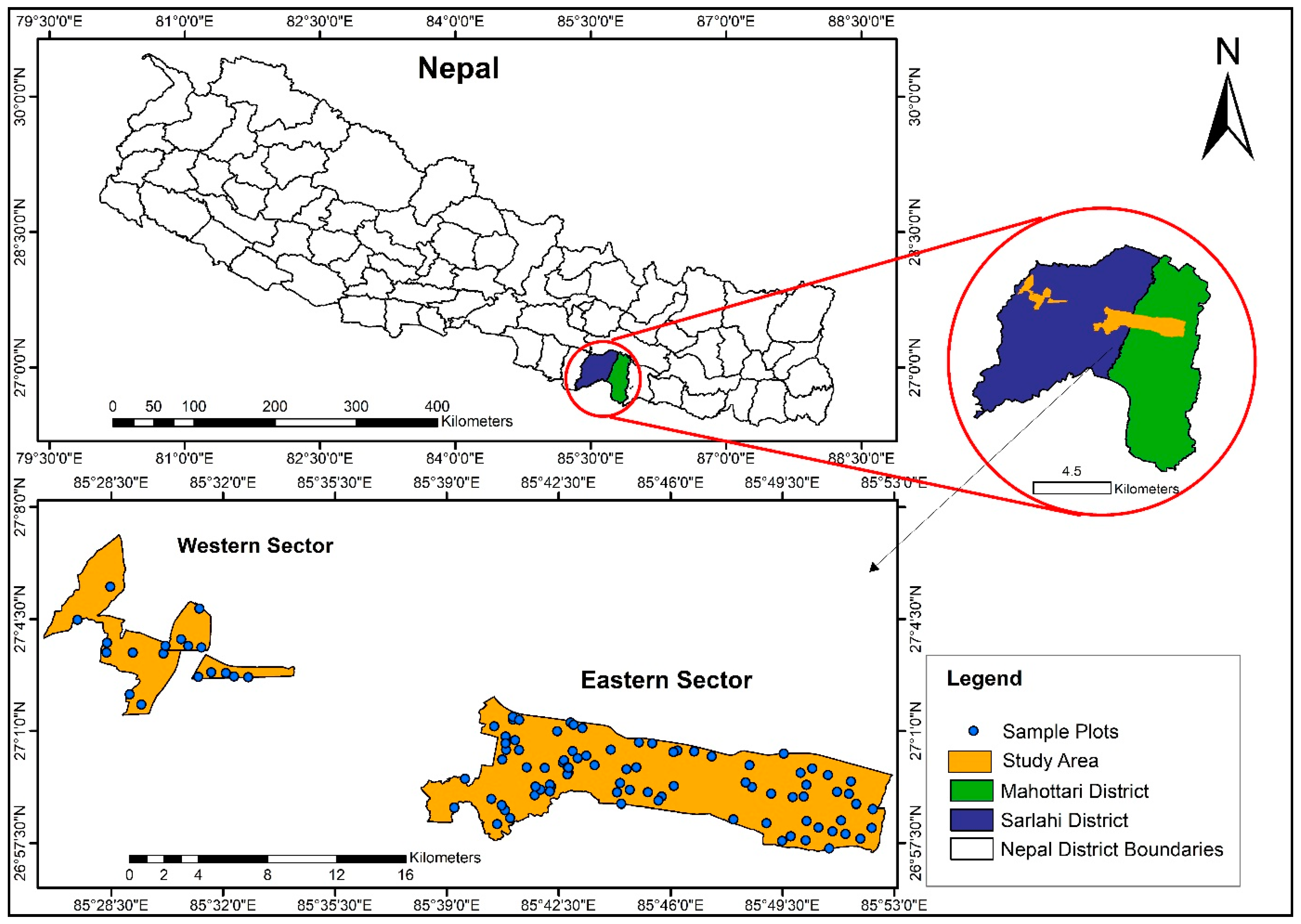
2.1. Study Area

The study area is situated within the Sagarnath Forest Development Project (SFDP) in the Central Terai region of Nepal (Figure 1), and it is located between 85°67′49″ east longitude and 26°99′74″ north latitude [54]. The government of Nepal manages the SFDP, established in 1985 on previously owned forest land. It covers a total area of 13,512 ha across two districts, namely Sarlahi and Mahottarai districts, in the lowland (Terai region) of Nepal. The total area consists of various land categories, including plantations (11,796 ha), natural forests (395 ha), protected forests (707 ha), and water bodies (615 ha). A large amount of Eucalyptus (Eucalyptus camaldulensis) and Teak (Tectona grandis) have been planted in the project area since its inception. The native forest type is characterized by mixed hardwood tropical forests, with Sal (Shorea robusta) being the dominant species, accounting for approximately 90% of the forest composition. The altitude in the Terai region ranges from 60 to 330 m above mean sea level. The climate in this region is characterized by hot summers, with temperatures ranging from 35 °C to 45 °C in April and May, and dry winters, with temperatures ranging from 10 °C to 15 °C in January. The region receives annual precipitation ranging from 1130 mm to 2680 mm [55]. The region consists of a piedmont plain formed by recent and post-Pleistocene alluvial deposits [45].

2.2. Field Measurements and AGB Estimates

Field data were collected from 110 circular inventory plots randomly distributed in the forest, each covering an area of 0.02 ha with a radius of 9 m. Tree attributes, including diameter at breast height (DBH), and tree height (H), were measured for every individual tree in each plot. Tree height was recorded using a Vertex III hypsometer, while diameters were measured using diameter tapes. The data collection was conducted in January 2021, and the GPS coordinates of the plot centers were also recorded. Out of the initial sampling design, 7 plots were excluded because they were located either on roads or inside riverbeds, and additionally, 13 plots visited in the field had no trees with a diameter of at least 5 cm for considering measurements. In the remaining sample plots, a total of 1138 trees with a DBH greater than or equal to 5 cm were measured. The total above-ground tree biomass (DBH > 5 cm) was obtained by summing up the stem biomass, branch biomass, and foliage biomass. Stem biomass was estimated by multiplying stem volume with the wood density of the species. The stem volume is determined using the equation developed by Sharma and Pukkala [56] for Nepalese tree species, which was used to compute stem volume. The stem volume equation for calculating the volume of trees is:
ln(v) = a + b × ln(DBH) + c × ln(H)
Here,
  • “v” is the volume per hectare (m3/ha);
  • “ln” is the natural logarithm with base 2.71828;
  • “DBH” is the diameter of trees at breast height (cm);
  • “H” is the height of trees (m).
  • Additionally, the coefficients a, b, and c are species-dependent.
The species wood density values for Nepalese tree species were obtained from Jackson [57]. Species-specific branch-to-stem biomass and foliage-to-stem biomass ratios were utilized to calculate branch and foliage biomasses from stem biomass [56]. Based on the corresponding plot area, the total AGB for each plot was then scaled to a per hectare (ton/ha) (Table 1).

2.3. LiDAR Data

The ALS LiDAR data were acquired by Geo3dModeling, a local vendor, using a helicopter in January 2021. The recorded LiDAR data were provided by Nepal Ban Nigam Limited, a governmental organization in Nepal. The LiDAR provided has a point density of at least 15 points per square meter. Using the LiDAR package version 4.0.3 in R 4.3.0 software, the LiDAR data were processed [58]. LiDAR data were normalized with a digital terrain model (DTM) of 1 m2 resolution to remove ground elevation from the height of returns. Subsequently, the point cloud data were clipped to the size of the field inventory sampling plots, ensuring that only relevant portions of the LiDAR data were retained for further analysis. Canopy density, which represents the ratio of vegetation to ground as observed from above, and canopy height, which measures the vertical distance between the top of the canopy and the ground, were calculated using the normalized point cloud and the clipped plots. These canopy height and canopy density metrics, along with the field inventory data from the plots, were combined for modeling purposes. The LiDAR metrics were computed at a resolution of 1 m2 and used as the predictor variables [54] (Table 2).

2.4. Above-Ground Biomass Mapping

Statistical techniques, such as random forest (RF) were used to establish a correlation between LiDAR point cloud data metrics and the above-ground biomass (AGB). The LiDAR metrics were considered independent variables, while AGB (ton/ha), which was determined at the plot level using field data, was the dependent variable.
RF is a powerful non-parametric machine learning algorithm that can be applied for both regression and classification [59]. The RF regression yields an arbitrary number of simple trees, which are a subset of independent variables–point cloud-derived metrics when estimating the dependent variable (AGB). The RF regression models are powerful for capturing complex, non-linear relationships between predictor variables (such as LiDAR metrics) and response variables (such as forest AGB). Unlike traditional linear regression models, the assumption of normality in the data is not necessary for RF regression [44].
We fitted the RF model using the ModelMap package in R [60]. This package utilizes the RF (random forest) function, a machine learning tool, to accurately capture the intricate and non-linear connections between LiDAR metrics and the AGB. This approach also allows for the determination of variable importance. RF utilizes bootstrap aggregation to create models that exhibit enhanced predictive abilities for estimation [61]. The estimation of AGB using the RF algorithm was carried out by considering two parameters: Mtry, which represents the number of predictor variables, and Ntree, which represents the number of decision trees. The function automatically optimizes Mtry parameter, denoting the number of randomly chosen variables at each node. For this specific case, the Ntree parameter was set to 500, indicating the quantity of trees grown in the model. The RF method was applied to estimate AGB using 32 point-derived metrics extracted from ALS LiDAR.
To assess the accuracy of AGB estimations, we split the inventory plots into two sets: a training dataset and a validation dataset. The data were randomly split at a ratio of 70:30, employing the createDataPartion function of the “caret” package [62]. The RF method was used in the R studio for modeling and accuracy evaluation [63]. The coefficient of determination (R2), root mean square error (RMSE), and MAE were applied to compare the performance of the RF algorithm [64,65]. The equation is as follows:
R 2 = 1 Y o b s , i Y ^ m o d , i 2 Y o b s , i Y ¯ o b s 2
R M S E = 1 n i = 1 n ( Y o b s , i Y ^ m o d , i ) 2
M A E = 1 N i = 1 N Y o b s , i Y ^ m o d , i
Here,
  • R 2 denotes the coefficient of determination;
  • Y o b s , i denotes the measured value;
  • Y ^ m o d , i denotes the model predicted value;
  • Y ¯ o b s denotes the average value;
  • n denotes the total number of samples;
  • R M S E denotes the root mean square error;
  • and MAE denotes the mean absolute error.
The “raster” package [66] in R was used to predict the spatial AGB in the study site. The “predict ()” function was employed, taking the raster dataset and the final model as inputs. The resulting AGB raster was utilized for the subsequent analysis process. Spatial grids of ALS metrics were generated for the study site at a resolution of 30 × 30 m. Using R 4.3.0 software, an AGB map was created with a spatial resolution of 30 × 30 m, utilizing LiDAR-derived variables obtained from ALS returns.

2.5. Climatic and Topographic Data

To assess the influence of environmental factors on AGB variability, climatic, topographic, soil, and land use land cover data were randomly collected for the 600 samples within the study area. Explanatory variables, including elevation, slope, aspect, land use land cover, and climate data such as mean annual temperature (MAT), and mean annual precipitation (MAP), were derived from geospatial datasets. Airborne LiDAR data were utilized to obtain high-resolution terrain information for the Earth’s surface with a resolution of 10 m (Table 3). For this process, a digital elevation model (DEM) was developed to obtain a digital representation of ground surface topography or terrain. Terrain variables were extracted from LiDAR ground points with a resolution of 10 m, as indicated in Table 3. The climatic variables, namely MAT (deg C) and MAP (mm) were obtained for the study sites from the Department of Hydrology and Meteorology (DHM) of Nepal (https://www.dhm.gov.np/, accessed on 5 September 2023), respectively. We created a 10 m resolution grid of mean annual precipitation (MAP) and mean annual temperature (MAT) data, monthly rainfall records, and temperature records of 11 ground stations in the study sites from 1981 to 2019 and interpolated using the ArcGIS 10.1 package. The land use land cover (LULC) types for the study area, with a resolution of 10 m, were acquired from ArcGIS online (https://livingatlas.arcgis.com/landcover/, accessed on 5 September, 2023). The soil type was extracted from the ICIMOD (International Centre for Integrated Mountain Development) in Nepal (https://rds.icimod.org/, accessed on 5 September 2023). Finally, both the AGB map and the explanatory variables were prepared into a 30 m × 30 m grid cell.

2.6. Statistical Model and Analysis

We used AGB as the dependent variable, while climatic, topographic, and soil variables were treated as independent variables for the statistical modeling. We employed the RF model to examine the relationship between AGB and the explanatory variables. We employed the random forest model (RF) in the R 4.3.0 software. The RF model, which utilizes machine learning algorithms based on decision trees, was utilized to assess the impact of various anthropogenic and environmental factors on AGB variability in managed forests [67]. The RF model is suitable for analyzing large datasets with numerous variables, accommodating both continuous and categorical variables, and demonstrating robustness against the multicollinearity problem [18]. We calculated the relative importance of potential predictor variables on AGB, calculating variable importance values using the RF algorithm [68,69]. The higher the percentage increase in mean square error (%IncMSE) and increase in nodePurity (IncNodePurity), the stronger the importance of these predictor variables.
In addition, the relative importance of variables was estimated using the mean decrease accuracy (MDA) metric used in the RF model. The MDA metric calculates the change in model accuracy on a test set by randomly shuffling the values of a feature, where a greater decrease in accuracy indicates a higher feature importance. We used the generated partial dependence plots to visualize the marginal effects of predictor variables on the response variable within the model. The partial plot function under the :randomForest” package version 4.7.1.1 in the R 4.3.0 software was used, following the methodology proposed by [70] Friedman (2001). Partial dependence plots are commonly employed to examine the linearity, non-linearity, or other intricate relationships between predictors and response variables [71].
These plots aid our analysis to assess the relationship between individual predictors and the response variable. To calculate the partial dependence function, we utilized the “pdp” R package version 0.8.1. The utilization of the partial dependence analysis results contributes to ascertaining the impact of individual variables on the response, while excluding the influence of other variables.

3. Results

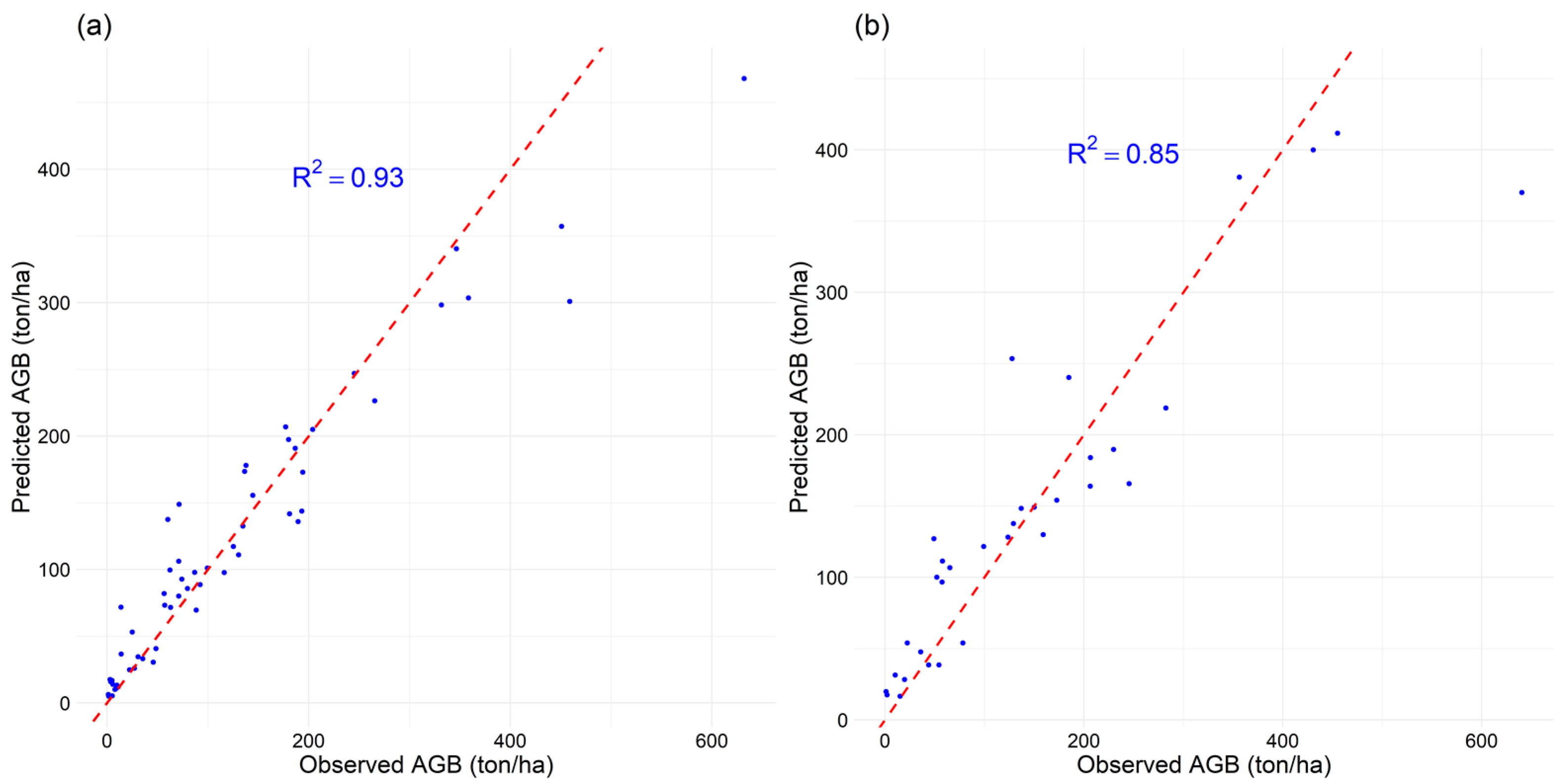
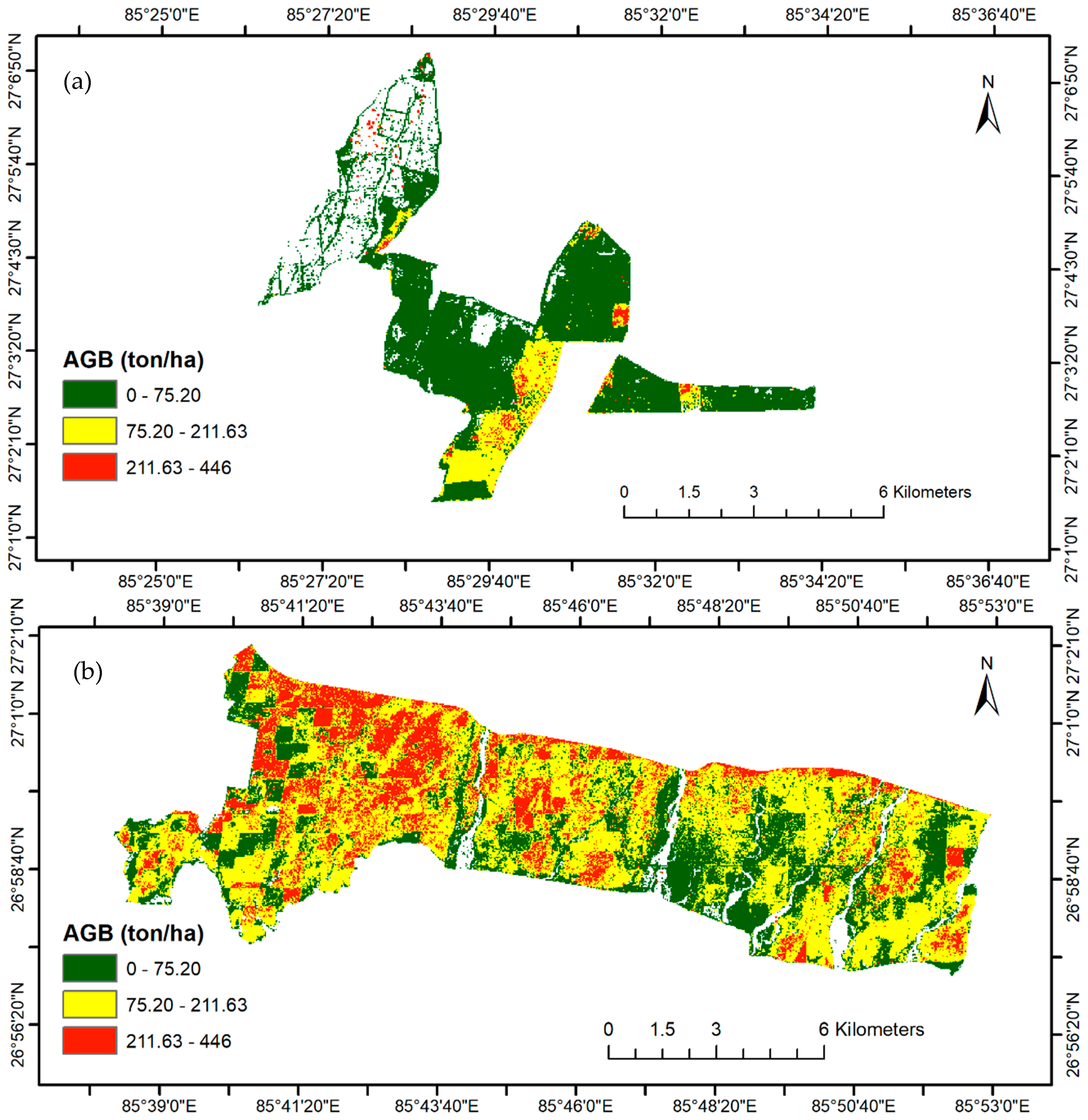
3.1. Aboveground Biomass—ALS Based Map

Independent variables in the RF model were derived from a total of 32 LiDAR-based metrics, which included zmax, zmean, zsd, zcv, zskew, zkurt, zentropy, pzabovemean, pzabove2, zq5, zq10, zq15, zq20, zq25, zq30, zq35, zq40, zq45, zq50, zq55, zq60, zq65, zq70, zq75, zq80, zq85, zq90, zq95, zpcum1, zpcum2, zpcum3, and CRR, respectively. The RF model calculated and plotted the variable importance, showing the top variables for AGB estimation (Figure 2).
However, among them, height-related metrics such as zmax, zmean, zq75, zq80, zq90, zq95, and density-based metrics, such as zpcum1, and zpcum2, exhibited relatively higher values for %IncMSE and IncNodepurity. It was found that zq95 and zmax were the most influential LiDAR metrics. Based on the training set, the model with the independent variables zmax, zmean, zq75, zq80, zq90, zq95, zpcum1, and zpcum2 achieved the best accuracy, with R2 of 0.93, RMSE of 38.45 ton/ha, and MAE of 25.06 ton/ha (Figure 3a). The model performance of the test data resulted in an accuracy of R2 of 0.85, RMSE of 60.9 ton/ha, and MAE of 39.7 ton/ha (Figure 3b). A visual representation of the relationship between predicted and observed values using a scatter plot is presented in Figure 3. This plot provides a visual comparison, allowing us to evaluate the models’ predictive capabilities for the training set and the test set using a random forest model.
Figure 4 illustrates the AGB map produced using the random forest model with a resolution of 30 × 30 m. The predicted AGB values in the study area varied from 0 to 446.42 ton/ha, with a mean value of 120 ton/ha. There is a noticeable variation in the spatial distribution of AGB within the study area. This distribution exhibited a distinct pattern, with AGB levels increasing from the east towards the center, and then decreasing further, highlighting the gradient of AGB levels across the study area (Figure 4). Parts of the eastern and western regions were characterized as low-value areas, with AGB levels recorded below 75.20 ton/ha. Parts of the southwestern and southeastern regions exhibited moderate AGB values, ranging between 75.20 and 211.63 ton/ha. Furthermore, most parts of the northcentral and northeastern regions displayed the highest AGB values, with values larger than 211.63 ton/ha. The spatial pattern of AGB within the study area demonstrated significant heterogeneity, with distinct variations observed across different regions.

3.2. Driving Factors of Aboveground Biomass

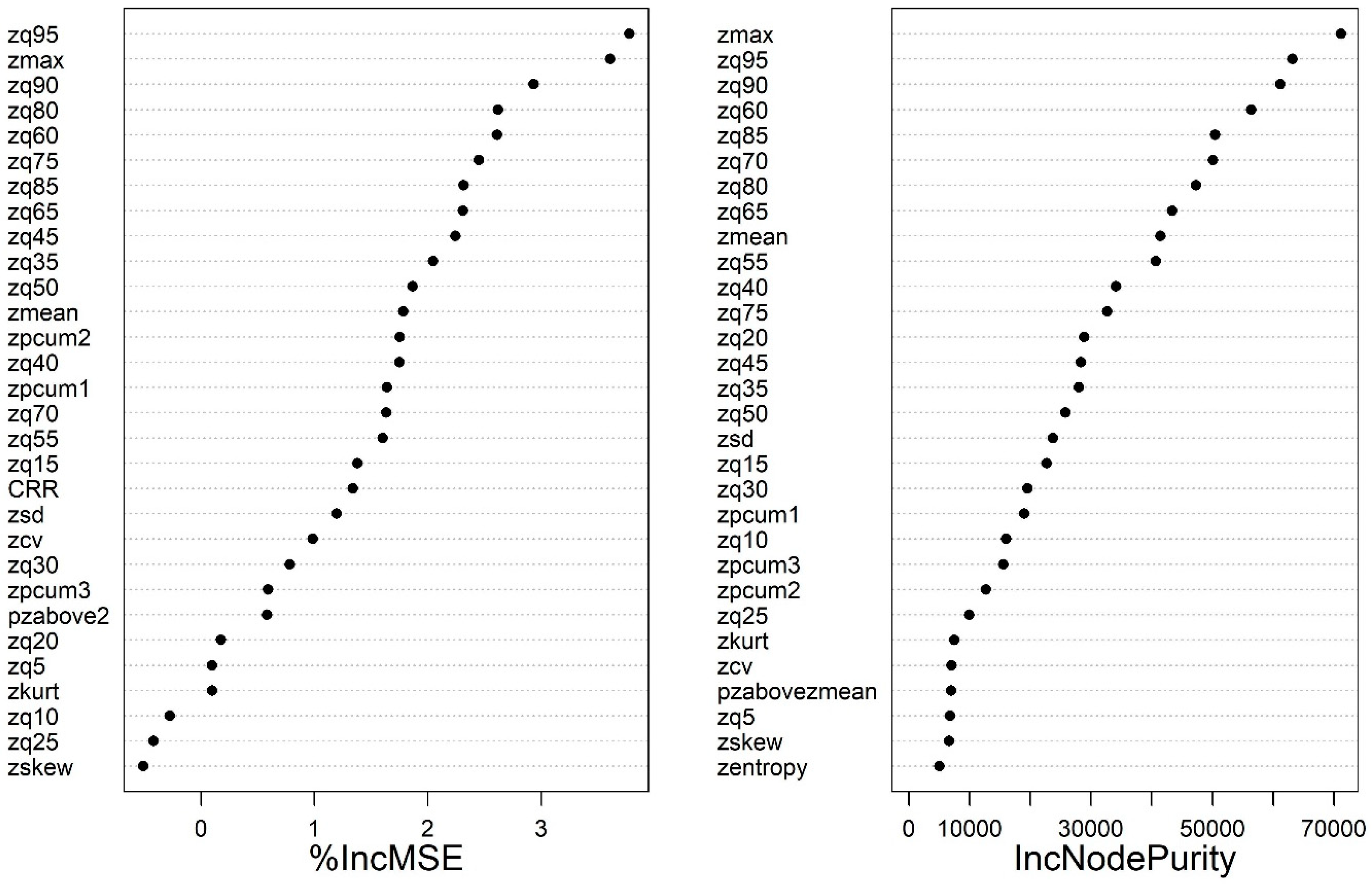
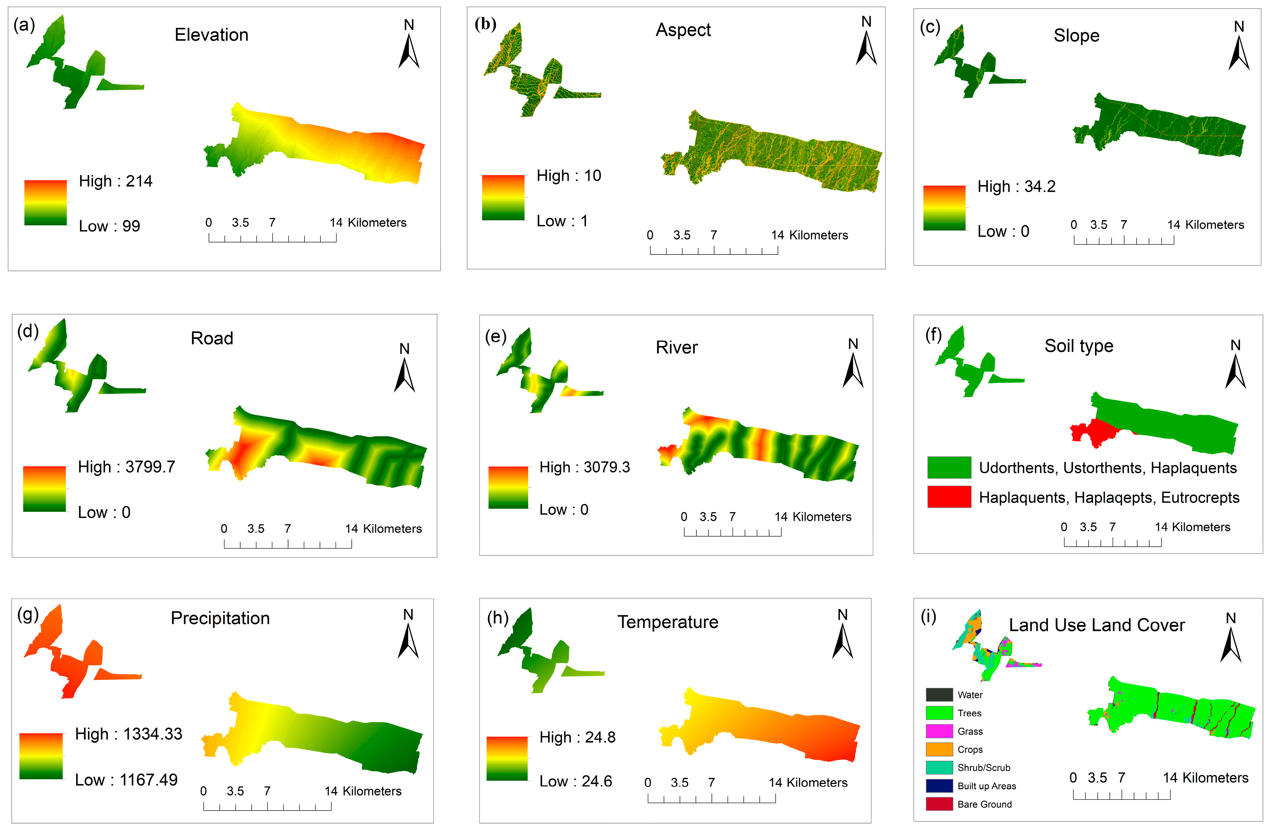
3.2.1. Variables Used in the RF Model

Figure 5 provides a visual representation of the explanatory variables used in our analysis. By examining these variables in relation to AGB, we aimed to gain a deeper understanding of the factors influencing the distribution of biomass in the study area.
In this study, the explanatory variables of the study area were in terms of climatic, topographic, soil, and land use land cover. The variables related to climate were mean annual precipitation (MAP) and mean annual temperature (MAT). MAP was mainly from 1167 mm to 1334 mm across the study area. MAT was between 24.6 and 24.8 degrees Celsius for the study area. Topographic variables included elevation, slope, and aspect. Elevations ranged from 99 m to 214 m. Slope ranging from 0 degrees to 34.2 degrees. Aspect refers to the direction in which slope faces, categorized into 10 ranges (0 = flat, 2 = north, 3 = northeast, 4 = east, 5 = southeast, 6 = south, 7 = southwest, 8 = west, 9 = northwest, 10 = north), respectively. Soil included soil type 2 (Udorthents, Ustorthents, and Haplaquents) and soil type 4 (Haplaquents, Haplaqepts, and Eutrocrepts). Anthropogenic variables included road distance and river distance. Road distance ranges from 0 to 3799.7 m. River distance ranging from 0 to 3079.3 m. LULC included water, trees, grass, crops, shrubs, built-up area, and bare ground, respectively.

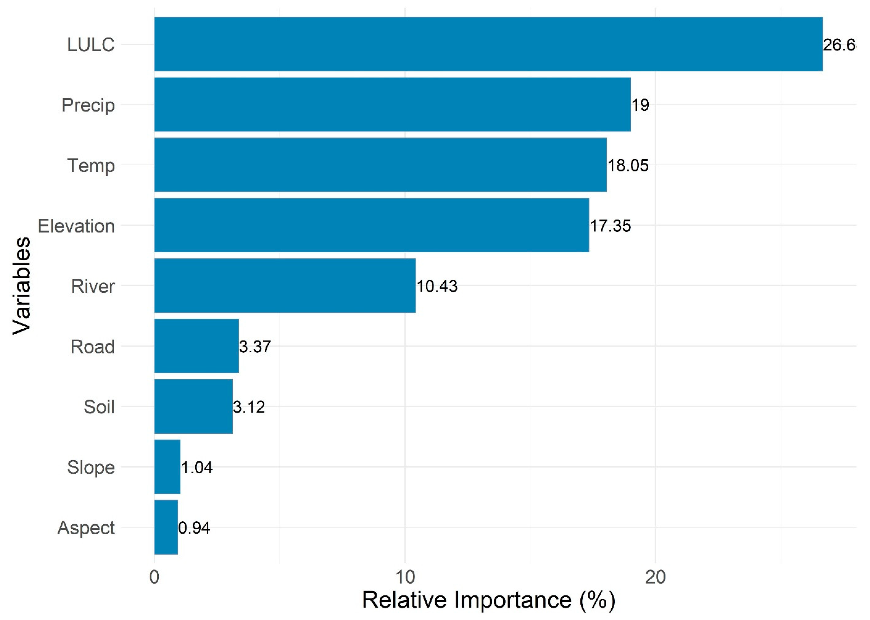
3.2.2. Relative Variables Importance in the RF Model

The selected nine environmental variables for explaining the spatial distribution of AGB, respectively, showed different relative importance values in the RF model (Figure 6). Predictor variables included: land use land cover (LULC), average annual precipitation (precip), average annual temperature (temp), elevation, river, soil, road, aspect, and slope, respectively (Figure 6). Among the variables, LULC, precipitation, and temperature emerged as the most influential factors, with relative importance percentages of 26.6%, 19%, and 18%, respectively. Elevation also played a significant role, with a percentage of 17.35%. Other variables (soil, river, road, slope, aspect) had lower relative importance percentages, ranging from 0.94% to 10.43%.

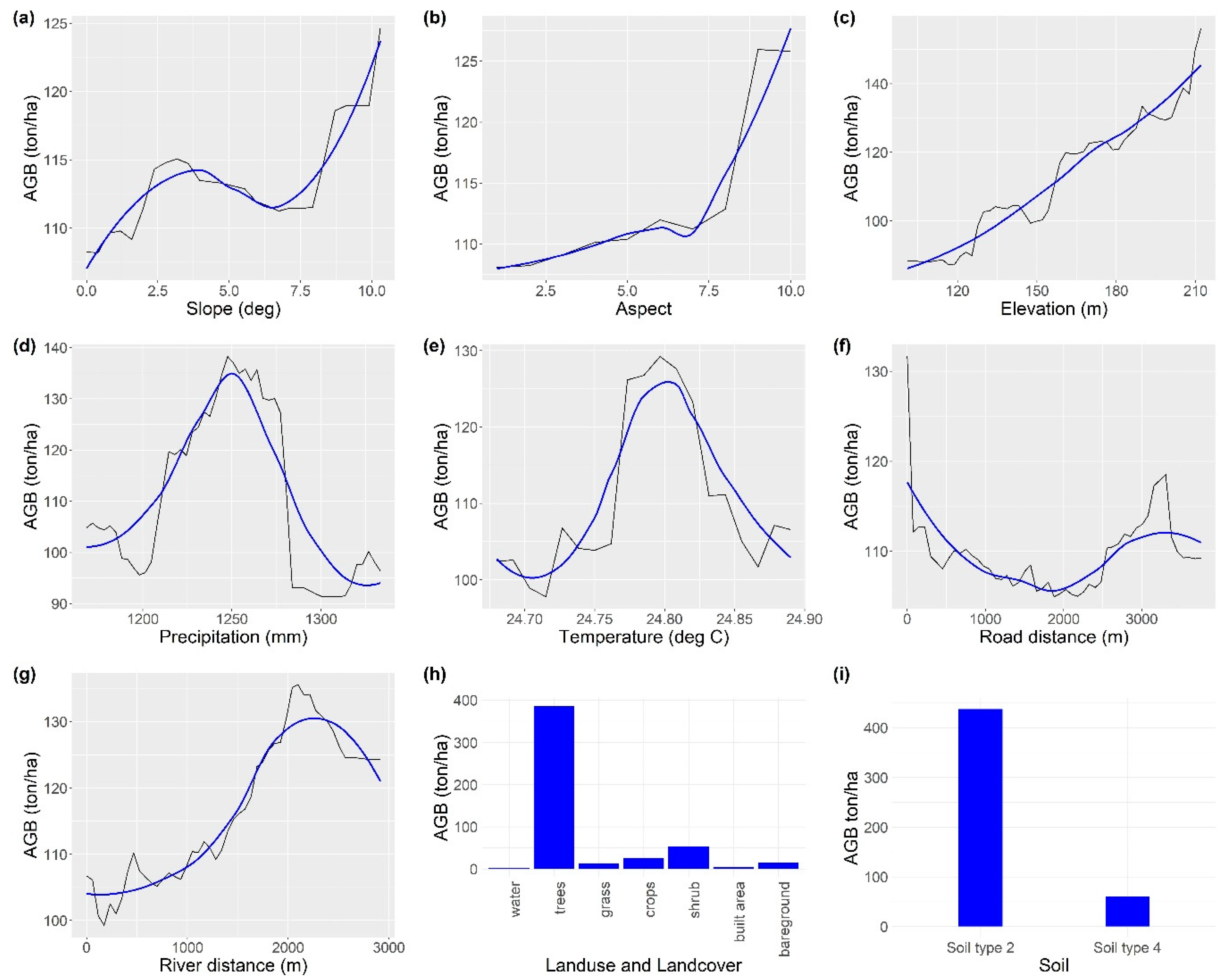
3.2.3. Partial Dependence Plots (Response Plots)

The factors used in the RF model contributed differently to the AGB in the study area, and their partial dependencies reflected their relationship to the AGB.
A single-variable partial dependence plot along with smoothed response curves for the explanatory variables is shown in Figure 7. The y-axis displays the fitted function for the response variable (AGB), and the model used is the random forest model. An increase in the distance to the road from the forests up to 2000 m contributed to the decrease in AGB, while an increase in AGB was found for longer distances. In contrast, river proximity up to 2000 m contributed to an increase in AGB, and afterward, it contributed to a decrease in AGB. An increase in precipitation up to 1250 mm contributed to the higher AGB, and a higher precipitation amount decreased the AGB. Similarly, an increase in temperature up to 24.80 degrees Celsius contributed to the increase in AGB, and after that, the variable decreased AGB. An increase in elevation and slope further increased AGB. The amount of AGB increased with aspects between 2.5 and 6, and then the amount of AGB stayed stable, while there was an increase in AGB between aspects 7.5 and 10. Soil type 2 (Udorthents, Ustorthents, and Haplaquents) contributed more to AGB than soil type 4 (Haplaquents, Haplaqepts, and Eutrocrepts). Lastly, the comparison of land use land cover types (water, tree, shrub, grass, crops, built-up area, and bare ground) revealed that trees contributed more to AGB, and bare ground contributed less to AGB.

4. Discussion

In our study, the random forest (RF) model was used to estimate and understand the variability and spatial distribution of AGB in the managed forest. Powell et al. [41] highlighted the RF model’s effectiveness, surpassing the performance of multiple linear regression. The application of the RF model not only provided estimates for predictor variables but also allowed for an assessment of their relative importance and the visualization of non-linear relationships through partial dependence plots (Figure 7). The RF model is capable of modeling non-linear relationships without requiring explicit assumptions about the functional form of the relationship and has been widely employed in forest AGB estimation [18]. The predicted AGB in the study varied from 0 to 446 ton/ha with a mean of 120 ton/ha, which closely aligned with the mean AGB of the field plots (Figure 4). However, the average AGB (120 ton/ha) of trees was lower than the AGB (190 ton/ha) estimated in the forest of the Terai region of Nepal [45]. This difference in estimates could be because the samples cover the entire Terai region and possibly a more mature forest with a more diverse species composition compared to our study site. Moreover, this study explained the spatial distribution of AGB using the AGB map and all the explanatory variables (Figure 4 and Figure 5). The spatial distribution of AGB values in the study area showed higher values in the northeast and southwest regions, gradually decreasing towards the northwest. The study found that the factors influencing the spatial pattern of AGB were not uniform throughout the entire study area. The variables such as land use land cover (LULC), precipitation, temperature, and elevation were identified as having higher relative importance percentages in explaining AGB patterns. Conversely, variables like slope and aspect had a lesser influence on AGB variation (Figure 6). The main factors influencing the variability in AGB distribution were found to be land use land cover, MAP, and MAT, collectively explaining 64% of the variability in AGB patterns (refer to Figure 6). The vegetation density, water availability, and temperature conditions emerge as essential factors significantly influencing AGB levels across our study area.
Past studies have highlighted the influence of various factors such as topography, species composition, climate, elevation, and soil fertility on the spatial distribution of aboveground biomass (AGB) at the regional scale [72,73,74,75,76]. In our study area, while considering land use land cover, the AGB increased with a higher percentage of land use land cover in managed forests, especially with trees. The increase in the number of trees is a result of reforestation efforts, such as planting trees in the harvested area (logging) and sustainable forest management practices, including selective logging (thinning), proper harvesting methods, and ensuring natural regeneration. These practices have led to the growth of new trees and promoted the growth and sustainability of forests, resulting in higher AGB. With regard to climatic variables, precipitation, and temperature explained non-linear effects on AGB in the study site, respectively (Figure 7). Bowman et al. [77,78] study in Australian temperate and subtropical eucalyptus forests found that plants require temperatures that encourage growth while minimizing transpiration or autotrophic respiration. This indicates the importance of maintaining optimal temperature conditions for plants to maximize their growth potential. Lewis et al. [79] found an increase in AGB in African tropical forests with precipitation during the driest nine months of the year and a decrease during the wettest three months of the year. Malla et al. [71] reported a positive effect on AGB of the precipitation of the driest month and the maximum temperature of the warmest month in the forests throughout Nepal. The positive effect of precipitation during the driest month suggests that ensuring water availability during periods of rainfall can contribute to increased growth in the growing season [36], resulting in higher AGB. Similarly, the positive influence of maximum temperature during the warmest months indicates the importance of favorable temperature conditions for promoting forest growth and forest biomass accumulation. The different climatic conditions can affect the dynamics of AGB throughout the year. Previous studies, together with our results, show that precipitation and temperature can have both positive and negative effects on the AGB distribution in forests. However, other factors, such as soil characteristics, nutrient availability, disturbance regimes, and species composition, also interact with temperature and precipitation to influence AGB patterns.
When considering slope, Du et al. [80] indicated that vegetation on higher slopes tends to experience less human disturbance, allowing these areas to be better preserved, fostering abundant forest growth, and promoting biomass accumulation. In terms of aspect, studies conducted by Fan et al. [81,82] have demonstrated that the south-, southwest-, west-, and northwest-facing slopes are often referred to as sunny slopes. These aspects receive a greater amount of sunlight, leading to increased rates of photosynthesis and greater vegetation productivity. As a result, the amount of AGB in these aspects tends to be higher compared to other aspects. Regarding elevation, higher elevations are often associated with cooler temperatures and increased moisture availability [42]. These favorable conditions create an environment conducive to plant growth and the accumulation of biomass. Furthermore, elevated regions may exhibit distinct soil characteristics, nutrient availability, and vegetation compositions, which can contribute to increased AGB levels.
In our study area, the AGB was most abundant at the higher altitudes, particularly in areas dominated by soil type 2 (comprising Udorthents, Usotorthents, and Haplaquents). These regions are less conducive to agricultural activities and have limited accessibility via road networks. Previous studies have also indicated a positive relationship between altitude and AGB in similar areas [34,83]. Similarly, Nepal et al. [84] reported increasing AGB of trees with increasing elevation in the subtropical forest of Nepal. The elevation gradient is associated with changes in temperature, precipitation, and forest-type succession [85]. The elevation of our research site, typically ranging from 99 to 214 m above sea level, suggests that a significant climate change is unlikely to occur. Contrary to the findings of many studies [86,87,88,89,90] that indicate a decline in AGB with increasing elevation, we observe an opposing trend. This discrepancy could be attributed to the relatively narrow range of elevation (99 m to 214 m) encompassing the forested areas within our study site.
Regarding the road feature, the presence of a road has a negative impact on AGB up to a certain distance, potentially due to factors such as increased human disturbance and land conversion near roads. However, beyond a specific threshold distance, the negative effects diminish, or other factors such as reduced human activity or improved environmental conditions lead to an increase in AGB. The contribution of distance to the nearest road is consistent with [91], who observed lower AGB in the distance from the forests to the road up to 2000 m, while higher AGB was found for longer distances. AGB distribution is likely to be higher in areas with less human disturbance [92,93].
Regarding rivers, the initial increase in AGB with proximity to rivers could be attributed to factors such as increased water availability, moisture gradient, nutrient deposition, or favorable soil conditions near riverbeds. These factors can promote plant growth and result in higher AGB. However, beyond the threshold, the decrease in AGB with increasing river distance suggests that other factors may come into play. These could include factors such as reduced water availability, increased competition for resources, or changes in soil properties farther away from the river. These conditions may lead to decreased vegetation growth and, consequently, lower AGB.
Soil properties play a significant role in influencing the AGB of tropical forests [39,79,94,95]. Various soil properties, such as pH, organic matter, total nitrogen, total phosphorus, and others, are analyzed to assess their impact. Within our study area, soil type 2 contributed more to AGB than soil type 4 (consisting of Haplaquents, Haplaqepts, and Eutrocrepts). The soil type 2 exhibits higher organic matter content, enhanced water-holding capacity, and improved nutrient availability [96], thereby fostering greater plant growth and biomass accumulation. Moreover, these soil types possess superior drainage and aeration properties, which facilitate root development and nutrient uptake. Conversely, soil type 4 exhibits lower organic matter content, diminished water retention capacity, and limited nutrient availability. These characteristics can impede plant growth and biomass production within these soil types. Our findings regarding the impact of soil on AGB align with previous studies. However, it is important to note that soil type alone may not be the sole determinant of AGB. Other factors, such as climate, topography, land use, and vegetation composition can also interact with soil type to influence AGB patterns. The complex interplay of these factors should be considered when understanding the dynamics of AGB in forest ecosystems.
It is crucial to understand the limitations of our study. Firstly, our investigation exclusively focused on managed forests in the Terai region of Nepal, which may limit the generalization of the findings to other forest types or areas. Additionally, we solely examined AGB and did not consider below-ground forest biomass. The study did not consider the influence of biotic factors such as forest types or stand age, which could also affect AGB in forests. While our results provide valuable insights, it is crucial to interpret them within the context of these limitations. Future studies should address these limitations to obtain a more comprehensive understanding of the subject matter.

5. Conclusions

The study examined the spatial patterns and influencing factors of forest aboveground biomass (AGB) in a managed forest in the Terai region of Nepal using geospatial and statistical techniques. The mean forest AGB in the study area was 120 ton/ha, with a range from 0 to 446 ton/ha in the 30 m resolution. AGB exhibited a higher distribution in the northeast and southeast regions, gradually decreasing towards the northwest. AGB positively correlated with elevation, slope, and distance from rivers, while it negatively correlated with proximity to roads. The increase in precipitation and temperature contributed to the initial rise in AGB, but beyond a certain lag, these variables led to a decline in AGB. Land use land cover, precipitation, and temperature predominantly contributed to the spatial distribution of AGB variation, accounting for 64% of the variability. The aspect had the least effect on AGB distribution. This study showed the influence of climate, land cover land use, and topography on the AGB pattern in the forest. With the help of the ALS-based AGB maps and various explanatory variables, it was possible to better understand the spatial pattern of AGB and the factors influencing AGB distribution across the managed forest. The results obtained from our study hold significant importance for making decisions about managing forests sustainably and mitigating climate change in the Terai region of Nepal. Understanding the factors that drive AGB variation such as climate, soil characteristics, species composition, and disturbance regimes, allows us to develop more accurate AGB, and predictions of forest productivity. The accuracy of the model can be improved further using larger forest biomass datasets and other explanatory variables.

Author Contributions

Y.B.K. was responsible for the research design, data collection, analysis, and manuscript writing. The conceptualization and supervision were conducted by Q.L. and H.A. The data visualization was conducted by C.X., P.S. and H.A. Each author made contributions to the data analysis, review, and editing. D.G. assisted with proofreading. All authors have read and agreed to the published version of the manuscript.

Funding

This research project was funded by the China Scholarship Council (CSC 2020SLJ017262). Open access funding was arranged by Forest Nepal.

Data Availability Statement

The data are not publicly available because they are intended to be protected before official publications and used in other ongoing research.

Acknowledgments

We would like to thank Nepal Ban Nigam Limited, Ministry of Forests and Environment, Government of Nepal, for providing us with the important data. We also thank the kind support of Arbonaut Ltd., Finland, for providing us with a copy of this data. We are grateful to Tribhuvan University, Institute of Forestry, Hetauda, Nepal. We also acknowledge the Key Laboratory for Silviculture and Conservation of the Ministry of Education, Beijing Forestry University, and International College of Beijing Forestry University, China, for providing us with optimal research conditions. Likewise, we thank to the University of Arkansas System Division of Agriculture, the University of Arkansas at Monticello, USA and the University of Helsinki, Finland for their support. We would like to thank Bikram Singh Thakuri, Subash Singh, and Animesh Poudel for their help.

Conflicts of Interest

The authors declare no conflict of interest.

References

  1. Goodale, C.L.; Apps, M.J.; Birdsey, R.A.; Field, C.B.; Heath, L.S.; Houghton, R.A.; Jenkins, J.C.; Kohlmaier, G.H.; Kurz, W.; Liu, S. Forest carbon sinks in the northern hemisphere. Ecol. Appl. 2002, 12, 891–899. [Google Scholar] [CrossRef]
  2. Woodbury, P.B.; Smith, J.E.; Heath, L.S. Carbon sequestration in the U.S. forest sector from 1990 to 2010. For. Ecol. Manag. 2010, 241, 14–27. [Google Scholar] [CrossRef]
  3. Pan, Y.; Birdsey, R.A.; Fang, J.; Houghton, R.; Kauppi, P.E.; Kurz, W.A.; Phillips, O.L.; Shvidenko, A.; Lewis, S.L.; Canadell, J.G.; et al. A large and persistent carbon sink in the world’s forests. Science 2011, 333, 988–993. [Google Scholar] [CrossRef] [PubMed]
  4. Cusack, D.F.; Axsen, J.; Shwom, R.; Hartzell-Nichols, L.; White, S.; Mackey, K.R.M. An interdisciplinary assessment of climate engineering strategies. Front. Ecol. Environ. 2014, 12, 280–287. [Google Scholar] [CrossRef] [PubMed]
  5. Kauranne, T.; Joshi, A.; Gautam, B.; Manandhar, U.; Nepal, S.; Peuhkurinen, J. LiDAR-assisted multi-source program (LAMP) for measuring above ground biomass and forest carbon. Remote Sens. 2017, 9, 154. [Google Scholar] [CrossRef]
  6. Urbazaev, M.; Thiel, C.; Cremer, F.; Dubayah, R.; Migliavacca, M.; Reichstein, M.; Schmullius, C. Estimation of forest aboveground biomass and uncertainties by integration of field measurements, airborne LiDAR, and SAR and optical satellite data in Mexico. Carbon Balance Manag. 2018, 13, 1–20. [Google Scholar] [CrossRef] [PubMed]
  7. Achard, F.; Eva, H.D.; Mayaux, P.; Stibig, H.J.; Belward, A. Improved Estimates of Net Carbon Emissions from Land Cover Change in the Tropics for the 1990s. Glob. Biogeochem. Cycles 2004, 18, 1–11. [Google Scholar] [CrossRef]
  8. Hese, S.; Lucht, W.; Schmullius, C.; Barnsley, M.; Dubayah, R.; Knorr, D.; Neumann, K.; Riedel, T.; Schröter, K. Global Biomass Mapping for an Improved Understanding of the CO2 Balance-the Earth Observation Mission Carbon-3D. Remote Sens. Environ. 2005, 94, 94–104. [Google Scholar] [CrossRef]
  9. Houghton, R.A. Aboveground Forest Biomass and the Global Carbon Balance. Glob. Chang. Biol. 2005, 11, 945–958. [Google Scholar] [CrossRef]
  10. Frolking, S.; Palace, M.W.; Clark, D.B.; Chambers, J.Q.; Shugart, H.H.; Hurtt, G.C. Forest Disturbance and Recovery: A General Review in the Context of Spaceborne Remote Sensing of Impacts on Aboveground Biomass and Canopy Structure. J. Geophys. Res. Biogeosciences 2009, 114, G00E02. [Google Scholar] [CrossRef]
  11. LeToan, T.S.; Quegan, M.; Davidson, W.J.; Balzter, H.; Paillou, P.; Papathanassiou, K.; Plummer, S. The BIOMASS Mission: Mapping Global Forest Biomass to Better Understand the Terrestrial Carbon Cycle. Remote Sens. Environ. 2011, 115, 2850–2860. [Google Scholar] [CrossRef]
  12. Lu, D. The potential and challenge of remote sensing-based biomass estimation. Int. J. Remote Sens. 2006, 27, 1297–1328. [Google Scholar] [CrossRef]
  13. Vashum, K.T.; Jayakumar, S. Methods to Estimate Above-Ground Biomass and Carbon Stock in Natural Forests—A Review. Ecosyst. Ecography 2012, 2, 1–7. [Google Scholar] [CrossRef]
  14. Du, L.; Zhou, T.; Zou, Z.; Zhao, X.; Huang, K.; Wu, H. Mapping forest biomass using remote sensing and national forest inventory in China. Forests 2014, 5, 1267–1283. [Google Scholar] [CrossRef]
  15. Tang, X.; Fehrmann, L.; Guan, F.; Forrester, D.; Guisasola, R.; Kleinn, C. Inventory based estimation of forest biomass in Shitai County, China: A comparison of five methods. Ann. For. Res. 2016, 59, 269–280. [Google Scholar] [CrossRef]
  16. Dang, A.T.N.; Nandy, S.; Srinet, R.; Luong, N.V.; Ghosh, S.; Senthil Kumar, A. Forest aboveground biomass estimation using machine learning regression algorithm in Yok Don National Park, Vietnam. Ecol. Inform. 2019, 50, 24–32. [Google Scholar] [CrossRef]
  17. Mura, M.; McRoberts, R.E.; Chirici, G.; Marchetti, M. Estimating and mapping forest structural diversity using airborne laser scanning data. Remote Sens. Environ. 2015, 170, 133–142. [Google Scholar] [CrossRef]
  18. Lu, D.; Chen, Q.; Wang, G.; Liu, L.; Li, G.; Moran, E. A survey of remote sensing-based aboveground biomass estimation methods in forest ecosystems. Int. J. Digit. Earth 2014, 9, 63–105. [Google Scholar] [CrossRef]
  19. Sačkov, I.; Santopuoli, G.; Bucha, T.; Lasserre, B.; Marchetti, M. Forest inventory attribute prediction using lightweight aerial scanner data in a selected type of multilayered deciduous forest. Forests 2016, 7, 12. [Google Scholar] [CrossRef]
  20. Lim, K.S.; Treitz, P.M. Estimation of above ground forest biomass from airborne discrete return laser scanner data using canopy-based quantile estimators. Scand. J. For. Res. 2004, 19, 558–570. [Google Scholar] [CrossRef]
  21. Hyyppä, J.; Hyyppä, H.; Xiaowei, Y.; Kaartinen, H.; Kukko, A.; Holopainen, M. Topographic Laser Ranging and Scanning: Principles and Processing; CRC Press Taylor & Francis Group: Boca Raton, FL, USA, 2009; pp. 335–370. [Google Scholar]
  22. Zhao, K.; Popescu, S. Lidar-based mapping of leaf area index and its use for validating GLOBCARBON satellite LAI product in a temperate forest of the southern USA. Remote Sens. Environ. 2009, 113, 1628–1645. [Google Scholar] [CrossRef]
  23. Birdsey, R.; Angeles-Perez, G.; Kurz, W.A.; Lister, A.; Olguin, M.; Pan, Y.; Wayson, C.; Wilson, B.; Johnson, K. Approaches to monitoring changes in carbon stocks for REDD+. Carbon Manag. 2013, 4, 519–537. [Google Scholar] [CrossRef]
  24. Subedi, M.; Matthews, R.; Pogson, M.; Abegaz, A.; Balana, B.; Oyesiku-blakemore, J.; Smith, J. ScienceDirect Can biogas digesters help to reduce deforestation in Africa ? Biomass Bioenergy 2014, 70, 87–98. [Google Scholar] [CrossRef]
  25. Law, B.E.; Turner, D.; Campbell, J.; Sun, O.J.; Van Tuyl, S.; Ritts, W.D.; Cohen, W.B. Disturbance and climate effects on carbon stocks and fluxes across Western Oregon USA. Glob. Chang. Biol. 2004, 10, 1429–1444. [Google Scholar] [CrossRef]
  26. Gough, C.M.; Vogel, C.S.; Harrold, K.H.; George, K.; Curtis, P.S. The legacy of harvest and fire on ecosystem carbon storage in a north temperate forest. Glob. Chang. Biol. 2007, 13, 1935–1949. [Google Scholar] [CrossRef]
  27. Hudiburg, T.; Law, B.; Turner, D.P.; Campbell, J.; Donato, D.; Duane, M. Carbon dynamics of Oregon and Northern California forests and potential land-based carbon storage. Ecol. Appl. 2009, 19, 163–180. [Google Scholar] [CrossRef] [PubMed]
  28. Hanberry, B.B.; He, H.S. Effects of historical and current disturbance on forest biomass in Minnesota. Landsc. Ecol. 2015, 30, 1473–1482. [Google Scholar] [CrossRef]
  29. Zhang, Y.; Gu, F.; Liu, S.; Liu, Y.; Li, C. Forest Ecology and Management Variations of carbon stock with forest types in subalpine region of southwestern China. For. Ecol. Manag. 2013, 300, 88–95. [Google Scholar] [CrossRef]
  30. Clark, K.L.; Gholz, H.L.; Castro, M.S. Carbon dynamics along a chronosequence of slash pine plantations in North Florida. Ecol. Appl. 2004, 14, 1154–1171. [Google Scholar] [CrossRef]
  31. Orihuela-Belmonte, D.E.; de Jong, B.H.J.; Mendoza-Vega, J.; van der Wal, J.; Paz-Pellat, F.; Soto-Pinto, L.; Flamenco-Sandoval, A. Carbon stocks and accumulation rates in tropical secondary forests at the scale of community, landscape and forest type. Agric. Ecosyst. Environ. 2013, 171, 72–84. [Google Scholar] [CrossRef]
  32. Yang, Y.; Watanabe, M.; Li, F.; Zhang, J.; Zhang, W.; Zhai, J. Factors affecting forest growth and possible effects of climate change in the Taihang Mountains, Northern China. Forestry 2006, 79, 135–147. [Google Scholar] [CrossRef]
  33. Ajaz Ahmed, M.A.; Abd-Elrahman, A.; Escobedo, F.J.; Cropper, W.P., Jr.; Martin, T.A.; Timilsina, N. Spatially-explicit modeling of multi-scale drivers of aboveground forest biomass and water yield in watersheds of the Southeastern United States. J. Environ. Manag. 2017, 199, 158–171. [Google Scholar] [CrossRef] [PubMed]
  34. Alves, L.F.; Vieira, S.A.; Scaranello, M.A.; Camargo, P.B.; Santos, F.A.M.; Joly, C.A.; Martinelli, L.A. Forest Ecology and Management Forest structure and live aboveground biomass variation along an elevational gradient of tropical Atlantic moist forest (Brazil). For. Ecol. Manag. 2010, 260, 679–691. [Google Scholar] [CrossRef]
  35. Asner, G.P.; Flint Hughes, R.; Varga, T.A.; Knapp, D.E.; Kennedy-Bowdoin, T. Environmental and biotic controls over aboveground biomass throughout a tropical rain forest. Ecosystems 2009, 12, 261–278. [Google Scholar] [CrossRef]
  36. Saud, J.; Lynch, P.; Cram, T.; Guldin, D. An Annual basal area growth model with multiplicative climate modifier fitted to longitudi-nal data for shortleaf pine. Forestry 2019, 92, 538–553. [Google Scholar] [CrossRef]
  37. Yan, Y.; Wu, F.; Wang, B. Estimating spatiotemporal patterns of aboveground biomass using Landsat TM and MODIS images in the Mu Us Sandy Land, China. Agric. For. Meteorol. 2015, 200, 119–128. [Google Scholar] [CrossRef]
  38. Tadese, S.; Soromessa, T.; Aneseye, A.B.; Gebeyehu, G. The impact of land cover change on the carbon stock of moist afromontane forests in the Majang Forest Biosphere Reserve. Carbon Balance Manag. 2023, 18, 24. [Google Scholar] [CrossRef] [PubMed]
  39. Hofhansl, F.; Chacón-Madrigal, E.; Fuchslueger, L.; Jenking, D.; Morera-Beita, A.; Plutzar, C. Climatic and edaphic controls over tropical forest diversity and vegetation carbon storage. Sci. Rep. 2020, 10, 5066. [Google Scholar] [CrossRef]
  40. RequenaSuarez, D.; Rozendaal, D.M.A.; De Sy, V.; Gibbs, D.A.; Harris, N.L.; Sexton, J.O. Variation in aboveground biomass in forests and woodlands in Tanzania along gradients in environmental conditions and human use. Environ. Res. Lett. 2021, 16, 044014. [Google Scholar] [CrossRef]
  41. Powell, S.L.; Cohen, W.B.; Healey, S.P.; Kennedy, R.E.; Moisen, G.G.; Pierce, K.B. Quantification of live aboveground forest biomass dynamics with Landsat time-series and field inventory data: A comparison of empirical modeling approaches. Remote Sens. Environ. 2010, 114, 1053–1068. [Google Scholar] [CrossRef]
  42. VanderLaan, C.; Verweij, P.A.; Quiñones, M.J.; Faaij, A.P.C. Analysis of biophysical and anthropogenic variables and their relation to the regional spatial variation of aboveground biomass illustrated for North and East Kalimantan, Borneo. Carbon Bal. Manag. 2014, 9, 8. [Google Scholar] [CrossRef] [PubMed]
  43. Rajput, B.S.; Bhardwaj, D.R.; Pala, N.A. Factors influencing biomass and carbon storage potential of different land use systems along an elevational gradient in temperate northwestern Himalaya. Agrofor. Syst. 2017, 91, 479–486. [Google Scholar] [CrossRef]
  44. Belgiu, M.; Csillik, O. Sentinel-2 cropland mapping using pixel-based and object-based time-weighted dynamic time warping analysis. Remote Sens. Environ. 2018, 204, 509–523. [Google Scholar] [CrossRef]
  45. DFRS. State of Nepal’s Forests; Department of Forest Research and Survey: Kathmandu, Nepal, 2015; ISBN 9789937889636. [Google Scholar]
  46. Kandel, P.N. Estimation of Above Ground Forest Biomass and Carbon Stock by Integrating Lidar, Satellite Image and Field Measurement in Nepal. J. Nat. Hist. Mus. 2015, 28, 160–170. [Google Scholar] [CrossRef]
  47. Murthy, M.S.R.; Wesselmann, S.; Hammad, G. Multi-Scale Forest Biomass Assessment and Monitoring in the Hindu Kush Himalayan Region: A Geospatial Perspective. Icimod 2008, 322, 202. [Google Scholar]
  48. Rana, P.; Popescu, S.; Tolvanen, A.; Gautam, B.; Srinivasan, S.; Tokola, T. Estimation of tropical forest aboveground biomass in Nepal using multiple remotely sensed data and deep learning. Int. J. Remote Sens. 2023, 44, 5147–5171. [Google Scholar] [CrossRef]
  49. Estornell, J.; Ruiz, L.A.; Velázquez-Martí, B.; Fernández-Sarría, A. Estimation of shrub biomass by airborne LiDAR data in small forest stands. Ecol. Manag. 2011, 262, 1697–1703. [Google Scholar] [CrossRef]
  50. Lefsky, M.A.; Cohen, W.B.; Harding, D.J.; Parker, G.G.; Acker, S.A.; Gower, S.T.; Service, F.; Way, S.W.J.; Goddard, N.; Flight, S. Lidar remote sensing of above-ground biomass in three biomes. Glob. Ecol. Biogeogr. 2002, 11, 393–399. [Google Scholar] [CrossRef]
  51. Li, Y.; Andersen, H.; Mcgaughey, R. A Comparison of Statistical Methods for Estimating Forest Biomass from Light Detection and Ranging Data. J. Appl. For. 2008, 23, 223–231. [Google Scholar] [CrossRef]
  52. Asner, G.P.; Mascaro, J. Mapping tropical forest carbon: Calibrating plot estimates to a simple LiDAR metric. Remote Sens. Environ. 2014, 140, 614–624. [Google Scholar] [CrossRef]
  53. Asner, G.P.; Powell, G.V.N.; Mascaro, J.; Knapp, D.E.; Clark, J.K.; Jacobson, J.K.; Bowdoin, T.; Balaji, A.; Paez-Acosta, G.; Victoria, E.; et al. High-resolution forest carbon stocks and emissions in the Amazon. Proc. Natl. Acad. Sci. USA 2010, 107, 16738–16742. [Google Scholar] [CrossRef] [PubMed]
  54. Kc, Y.B.; Liu, Q.; Saud, P.; Gaire, D.; Adhikari, H. Estimation of Above-Ground Forest Biomass in Nepal by the Use of Airborne LiDAR, and Forest Inventory Data. Land 2024, 13, 213. [Google Scholar] [CrossRef]
  55. FRA/DFRS. Forest Resource Assessment Nepal Project/Department of Forest Research and Survey; FRA/DFRS: Babarmahal, Kathmandu, 2014. [Google Scholar]
  56. Sharma, E.R.; Pukkala, T. Volume Equations and Biomass Prediction of Forest Trees in Nepal; ResearchGate: Berlin, Germany, 1990. [Google Scholar]
  57. Jackson, J.K. Afforestation, Manual of Forest, in Nepal, 2nd ed.; Research and Survey Center: Kathmandu, Nepal, 1994; Volume I. [Google Scholar]
  58. Roussel, J.R.; Auty, D.; Coops, N.C.; Tompalski, P.; Goodbody, T.R.H.; Meador, A.S.; Bourdon, J.F.; de Boissieu, F.; Achim, A. lidR: An R package for analysis of Airborne Laser Scanning (ALS) data. Remote Sens. Environ. 2020, 251, 112061. [Google Scholar] [CrossRef]
  59. Fawagreh, K.; Gaber, M.M.; Elyan, E. Systems Science & Control Engineering: An Open Access Random forests: From early developments to recent advancements. Syst. Sci. Control. Eng. Open Access J. 2014, 2583, 602–609. [Google Scholar] [CrossRef]
  60. Freeman, A.E.; Frescino, T.; Moisen, G.G. ModelMap: An R Package for Model Creation and Map Production; R Package Version 4; R Foundation for Statistical Computing: Vienna, Austria, 2023; pp. 6–12. [Google Scholar]
  61. Pandit, S.; Tsuyuki, S.; Dube, T. Estimating above-ground biomass in sub-tropical buffer zone community forests, Nepal, using Sentinel 2 data. Remote Sens. 2018, 10, 601. [Google Scholar] [CrossRef]
  62. Kuhn, M. Building Predictive Models in R Using the caret Package. J. Stat. Softw. 2008, 28, 1–26. [Google Scholar] [CrossRef]
  63. R Core Team R. A Language and Environment for Statistical Computing. R Foundation for Statistical Computing, Vienna. Available online: www.R-project.org (accessed on 5 September 2023).
  64. Vafaei, S.; Soosani, J.; Adeli, K.; Fadaei, H.; Naghavi, H.; Pham, T.D.; Bui, D.T. Improving accuracy estimation of Forest Aboveground Biomass based on incorporation of ALOS-2 PALSAR-2 and Sentinel-2A imagery and machine learning: A case study of the Hyrcanian forest area (Iran). Remote Sens. 2018, 10, 172. [Google Scholar] [CrossRef]
  65. Jiang, X.; Li, G.; Lu, D.; Chen, E.; Wei, X. Stratification-based forest aboveground biomass estimation in a subtropical region using airborne lidar data. Remote Sens. 2020, 12, 1101. [Google Scholar] [CrossRef]
  66. Van Etten, J.; Sumner, M.; Cheng, J.; Baston, D.; Bevan, A.; Bivand, R.; Busetto, L.; Canty, M.; Fasoli, B.; Forrest, D.; et al. Package ‘raster’ R topics documented. R Package 2023, 734, 473. [Google Scholar]
  67. Jin, Z.; Shang, J.; Zhu, Q.; Ling, C.; Xie, W.; Qiang, B. RFRSF: Employee Turnover Prediction Based on Random Forests and Survival Analysis. In Proceedings of the Lecture Notes in Computer Science (Including Subseries Lecture Notes in Artificial Intelligence and Lecture Notes in Bioinformatics), Fisciano, Italy, 29 June–3 July 2020. [Google Scholar]
  68. Breiman, L. Random Forests. Mach. Learn. 2001, 45, 5–32. [Google Scholar] [CrossRef]
  69. Liaw, A.; Wiener, M. Classification and Regression by randomForest. R News 2002, 2, 18–22. [Google Scholar]
  70. Friedman, J.H. Greedy function approximation: A gradient boosting machine. Ann. Stat. 2001, 29, 1189–1232. [Google Scholar] [CrossRef]
  71. Malla, R.; Neupane, P.R.; Köhl, M. Assessment of above ground biomass and soil organic carbon in the forests of Nepal under climate change scenario. Front. For. Glob. Change 2023, 6, 1209232. [Google Scholar] [CrossRef]
  72. Ali, A.; Lin, S.L.; He, J.K.; Kong, F.M.; Yu, J.H.; Jiang, H.S. Climate and soils determine aboveground biomass indirectly via species diversity and stand structural complexity in tropical forests. For. Ecol. Manag. 2019, 432, 823–831. [Google Scholar] [CrossRef]
  73. Yuan, S.; Tang, T.; Wang, M.; Chen, H.; Zhang, A.; Yu, J. Regional Scale Determinants of Nutrient Content of Soil in a Cold-Temperate Forest. Forests 2018, 9, 177. [Google Scholar] [CrossRef]
  74. Slik, J.W.F.; Paoli, G.; Mcguire, K.; Amaral, I.; Barroso, J.; Bastian, M.; Blanc, L.; Bongers, F.; Boundja, P.; Clark, C.; et al. Large trees drive forest aboveground biomass variation in moist lowland forests across the tropics. Glob. Ecol. Biogeogr. 2013, 22, 1261–1271. [Google Scholar] [CrossRef]
  75. Liu, L.; Lim, S.; Shen, X.; Yebra, M. Assessment of generalized allometric models for aboveground biomass estimation: A case study in Australia. Comput. Electron. Agric. 2020, 175, 105610. [Google Scholar] [CrossRef]
  76. Laurance, W.F.; Fearnside, P.M.; Laurance, S.G.; Lovejoy, T.E.; Merona, J.M.R.; Jeffrey, Q.; Gascon, C. Relationship between soils and Amazon forest biomass: A landscape-scale study. For. Ecol. Manag. 1999, 118, 127–138. [Google Scholar] [CrossRef]
  77. Bowman, D.; Williamson, K.; Prior, L. A warmer world will reduce tree growth in evergreen broadleaf forests: Evidence from Australian temperate and subtropical eucalypt forests. Glob. Ecol. Biogeogr. 2014, 23, 925–934. [Google Scholar] [CrossRef]
  78. Medlyn, B.; Zeppel, M.; Brouwers, N.; Howard, K.; Gara, E.; Hardy, G.; Lyons, T.; Li, L.; Evans, B. An Assessment of the Vulnerability of Australian Forests to the Impacts of Climate Change; Griffith University: Brisbane, Australian, 2011. [Google Scholar]
  79. Lewis, S.L.; Sonké, B.; Sunderland, T.; Begne, S.K.; Lopez-Gonzalez, G.; van der Heijden, G.M.F.; Phillips, O.L.; Affum-Baffoe, K.; Baker, T.R.; Banin, L.; et al. Above-ground biomass and structure of 260 African tropical forests. Philos. Trans. R. Soc. B Biol. Sci. 2013, 368, 295. [Google Scholar] [CrossRef]
  80. Du, Q.; Xu, J.; Wang, J.; Zhang, F.; Ji, B. Correlation between forest carbon distribution and terrain elements of altitude and slope. J. Zhejiang A F Univ. 2013, 30, 330–335. [Google Scholar]
  81. Fan, Y.; Zhou, G.; Shi, Y.; Du, H.; Zhou, Y.; Xu, X. Effects of terrain on stand structure and vegetation carbon storage of phyllostachys edulis forest. Sci. Silvae Sin. 2013, 49, 177–182. [Google Scholar]
  82. Li, P.; Wei, X.; Tang, M. Forest site classification based on nfi and dem in zhejiang province. J. Southwest For. Univ. 2018, 38, 137–144. [Google Scholar]
  83. De Castilho, C.V.; Magnusson, W.E.; de Araújo, R.N.O.; Luizão, R.C.C.; Luizão, F.J.; Lima, A.P.; Higuchi, N. Variation in aboveground tree live biomass in a central Amazonian Forest: Effects of soil and topography. For. Ecol. Manag. 2006, 234, 85–96. [Google Scholar] [CrossRef]
  84. Nepal, S.; Kc, M.; Pudasaini, N.; Adhikari, H. Divergent Effects of Topography on Soil Properties and Above-Ground Biomass in Nepal’s Mid-Hill Forests. Resources 2023, 12, 136. [Google Scholar] [CrossRef]
  85. Sanaei, A.; Ali, M.; Chahouki, Z.; Ali, A.; Jafari, M.; Azarnivand, H. Science of the Total Environment Abiotic and biotic drivers of aboveground biomass in semi-steppe rangelands. Sci. Total Environ. 2018, 615, 895–905. [Google Scholar] [CrossRef] [PubMed]
  86. Raich, J.W.; Russell, A.E.; Vitousek, P.M. Primary productivity and ecosystem development along an elevational gradient on Mauna Loa, Hawaii. Ecology 1997, 78, 707–721. [Google Scholar]
  87. Waide, R.B.; Zimmerman, J.K.; Scatena, F.N. Controls of primary productivity: Lessons from the Luquillo Mountains in Puerto Rico. Ecology 1998, 79, 31–37. [Google Scholar] [CrossRef]
  88. Aiba, S.; Kitayama, K. Structure, composition and species diversity in an altitude-substrate matrix of rain forest tree communities on Mount Kinabalu, Borneo. Plant Ecol. 1999, 140, 139–157. [Google Scholar] [CrossRef]
  89. Kitayma, K.; Aiba, S. Ecosystem structure and productivity of tropical rain forests along altitudinal gradients with contrasting soil phosphorus pools on Mount Kinabalu, Borneo. J. Ecol. 2002, 90, 37–51. [Google Scholar] [CrossRef]
  90. Leuschner, C.; Moser, G.; Bertsch, C.; Röderstein, M.; Hertel, D. Large altitudinal increase in tree root/shoot ratio in tropical mountain forests of Ecuador. Basic Appl. Ecol. 2007, 8, 219–230. [Google Scholar] [CrossRef]
  91. Broich, M.; Hansen, M.; Stolle, F.; Potapov, P.; Margono, B.A.; Adusei, B. Remotely sensed forest cover loss shows high spatial and temporal variation across Sumatera and Kalimantan, Indonesia 2000–2008. Environ. Res. Lett. 2011, 6, 014010. [Google Scholar] [CrossRef]
  92. Mehta, V.K.; Sullivan, P.J.; Walter, M.T.; Krishnaswamy, J.; Degloria, S.D. Impacts of disturbance on soil properties in a dry tropical forest in Southern India. Ecohydrology 2008, 175, 161–175. [Google Scholar] [CrossRef]
  93. Rad, J.E.; Valadi, G.; Salehzadeh, O.; Maroofi, H. Effects of anthropogenic disturbance on plant composition, plant diversity and soil properties in oak forests, Iran. J. For. Sci. 2018, 2018, 358–370. [Google Scholar]
  94. Ma, L.; Li, W.; Shi, N.; Fu, S.; Lian, J.; Ye, W. Temporal and spatial patterns of aboveground biomass and its driving forces in a subtropical forest: A case study. Pol. J. Ecol. 2019, 67, 95–104. [Google Scholar] [CrossRef]
  95. Oberleitner, F.; Egger, C.; Oberdorfer, S.; Dullinger, S.; Wanek, W.; Hietz, P. Forest Ecology and Management Recovery of aboveground biomass, species richness and composition in tropical secondary forests in SW Costa Rica. For. Ecol. Manag. 2021, 479, 118580. [Google Scholar] [CrossRef]
  96. Ojha, R.B.; Panday, D. (Eds.) The Soils of Nepal; Springer International Publishing: Berlin/Heidelberg, Germany, 2021. [Google Scholar]
Figure 1. Study area location, and the distribution of the sampling plots.
Forests 15 00663 g001
Figure 2. Variable importance ranking for the AGB estimation RF model.
Forests 15 00663 g002
Figure 3. Scatterplot displaying correlation between observed and predicted AGB values for the training set (a) and the test set (b), using the best selected RF model.
Forests 15 00663 g003
Figure 4. ALS AGB map based on the RF model: (a) Western sector and (b) Eastern sector.
Forests 15 00663 g004
Figure 5. Environmental variables map for input determinant variables: (ai) explanatory variables at 30 × 30 m resolution: (a) elevation, (b) aspect, (c) slope, (d) road, (e) river, (f) soil type, (g) average annual precipitation, (h) average annual temperature, and (i) land use land cover.
Forests 15 00663 g005
Figure 6. Relative importance of variables, percentage, for AGB distribution using the RF model.
Forests 15 00663 g006
Figure 7. The partial dependence plot of the RF model, for each explanatory variable: (a) AGB and slope, (b) AGB and aspect, (c) AGB and elevation, (d) AGB and precipitation, (e) AGB and temperature, (f) AGB and road distance, (g) AGB and river distance, (h) AGB and land use land cover, and (i) AGB and soil. In (ag), the black line represents the partial dependence plot based on the random forest predictions, and the blue line represents the LOESS smoothed line.
Forests 15 00663 g007
Table 1. Summary of plot-level inventory plots.
AttributesMean ± Standard DeviationRange (Minimum to Maximum)
Density (trees/ha)462 ± 34339–2122
DBH (cm)24 ± 146–101
Height (m)17 ± 72–28
Basal area (m2)12 ± 100.2–47
Volume (m3/ha)108 ± 1120.6–519
AGB (ton/ha)131 ± 1371–640
Table 2. Predictor variables extracted from ALS-LiDAR metrics (height, density, and canopy) for modeling the AGB.
ALS- LiDAR MetricsPredictor VariablesCharacteristics
Height metricsPercentiles height (zq5 to zq95)Percentiles of the ALS height distributions, where the “z” typically stands for height and “q” stands for quantile or percentile (including 5th, 10th, 15th, 20th, 25th, 30th, 35th, 40th, 45th, 50th, 55th, 60th, 65th, 70th, 75th, 80th, 85th, 90th, 95th) for all points above 2 m
Maximum heights (zmax)Maximum heights above 2 m for all points
Mean heights (zmean)Mean heights above 2 m for all points
Coefficient of variation of height (zcv)Coefficient of variation of heights for all points above 2 m
Standard deviation (zsd)Standard deviation of heights for all points above 2 m
Skewness (zskew)Skewness of heights for all points above 2 m
Kurtosis (zkurt)Kurtosis of the heights for all points above 2 m
Entropy (zentropy)Entropy of the height distribution
Density metricspzabove2Percentages of first returns above 2 m
pzabovezmeanPercentage of returns greater than the mean returns height
zpcum1Cumulative percentage of first returns in the lower 10% of maximum elevation
zpcum2Cumulative percentage of first returns in the lower 20% of maximum elevation
zpcum3Cumulative percentage of first returns in the lower 30% of maximum elevation
Relative shape of the canopyCanopy relief ratio (CRR)Calculated as (height mean-height min)/(height max-height min), which represents the relative shape of the canopy
Table 3. Description of explanatory variables related to environmental factors.
Variable TypeDescriptionSpatial Resolution Data Source
Climatic variablesMean annual temperature (deg C) from 1981 to 202110 m × 10 mDHM (http://www.dhm.gov.np/, accessed on 5 September 2023)
Mean annual precipitation (mm)
from 1981 to 2021
10 m × 10 m
Topographic and soil variablesElevation (m a.s.l.) based on DEM10 m × 10 mDEM-LiDAR
Slope (deg) based on DEM10 m × 10 mDEM-LiDAR
Aspect (deg) based on DEM10 m × 10 mDEM-LiDAR
Soil type10 m × 10 mICIMOD (https://rds.icimod.org/home/datadetail?metadataid=1889, accessed on 5 September 2023)
Road distance10 m × 10 mICIMOD (https://rds.icimod.org/home/datadetail?metadataid=1889, accessed on 5 September 2023)
River distance10 m × 10 mICIMOD (https://rds.icimod.org/home/datadetail?metadataid=1889, accessed on 5 September 2023)
Land use land cover Sentinel-2: Land Use/Land Cover 2021 10 m × 10 mArcGIS online (https://livingatlas.arcgis.com/landcover/, accessed on 5 September 2023)
Disclaimer/Publisher’s Note: The statements, opinions and data contained in all publications are solely those of the individual author(s) and contributor(s) and not of MDPI and/or the editor(s). MDPI and/or the editor(s) disclaim responsibility for any injury to people or property resulting from any ideas, methods, instructions or products referred to in the content.

