Article

Insights into Canopy Escape Ratio from Canopy Structures: Correlations Uncovered through Sentinel-2 and Field Observation

1
Forest ICT Research Center, National Institute of Forest Science, Seoul 02455, Republic of Korea
2
Department of Civil, Urban, Earth, and Environmental Engineering, Ulsan National Institute of Science and Technology, Ulsan 44919, Republic of Korea
3
Graduate School of Carbon Neutrality, Ulsan National Institute of Science and Technology, Ulsan 44919, Republic of Korea
*
Author to whom correspondence should be addressed.
Forests 2024, 15(4), 665; https://doi.org/10.3390/f15040665
Submission received: 5 March 2024 / Revised: 30 March 2024 / Accepted: 5 April 2024 / Published: 7 April 2024
(This article belongs to the Section Forest Inventory, Modeling and Remote Sensing)

Abstract

:
This study explores the quantitative relationship between canopy structure and the canopy escape ratio (fesc), measured as the ratio of near-infrared reflectance of vegetation (NIRv) to the fraction of absorbed photosynthetically active radiation (fAPAR). We analyzed the correlation between fesc and key indicators of canopy structure—specifically, leaf area index (LAI) and clumping index (CI)—utilizing both Sentinel-2 satellite data and in situ observations. Our analysis revealed a moderate correlation between fesc and LAI, evidenced by an R2 value of 0.37 for satellite-derived LAI, which contrasts with the lower correlation (R2 of 0.15) observed with field-measured LAI. Conversely, the relationship between fesc and CI proved to be significantly weaker (R2 < 0.1), indicating minimal interaction between foliage distribution and light escape at the canopy level. This disparity in correlation strength was further evidenced in time series analysis, which showed little phenological variation in fesc compared to LAI. Our findings elucidate the complexities of estimating fesc based on the NIRv to fAPAR ratio and underscore the need for advanced methodologies in future research to enhance the accuracy of canopy escape models.

1. Introduction

The near-infrared reflectance of vegetation (NIRv) presents a new opportunity for the reliable physical interpretation of photosynthesis in terrestrial ecosystems. NIRv, which is derived from multiplying near-infrared reflectance with the normalized difference vegetation index (NDVI), effectively captures the combined influence of leaf and canopy structure on light absorption [1]. NIRv has shown a higher correlation with gross primary productivity (GPP) than NDVI [1,2,3]. Numerous studies have demonstrated that such a robust correlation [4,5] can substantially improve GPP estimation using NIRv and its derivatives, such as NIRvP [6,7]. The simplicity and intuitiveness of NIRv have led to its application in various forms of vegetation research, such as GPP estimation [5,8], long-term trend analysis [9,10], and climate–vegetation interactions [4,11].
The relationship between NIRv and canopy structure is critical for deepening our understanding of ecosystem dynamics and enhancing vegetation monitoring and GPP estimations. NIRv is influenced by canopy structure on light absorption, transmittance, and reflectance due to different leaf and canopy configurations such as leaf area index (LAI), leaf orientation, and foliage clumping [1]. This suggests that NIRv, sensitive to canopy structure, exhibits greater spatial variability in canopy configurations than that observed in NDVI. For example, the variability of NIRv, fluorescence correction vegetation index (FCVI), and enhanced vegetation index (EVI) was most noticeable at spatial scales of approximately 50 m, which is smaller than that in NDVI (approximately 90 m) [12]. In addition, [13] also demonstrated little saturation between NIRv and canopy photosynthesis, even at low LAI values. In this way, recent studies have used NIRv as a structural indicator in various areas, such as plant phenology [14,15,16,17], crop yield estimation [18], and drought stress assessment [19,20].
The NIRvP, which is NIRv multiplied by photosynthetically active radiation (PAR), is recognized as a potent proxy for structural solar-induced chlorophyll fluorescence (SIF) [6]. Given that SIF is a byproduct of light reactions in photosynthesis, numerous studies have endeavored to elucidate the physiological mechanisms linking SIF and GPP [21,22]. At large spatiotemporal scales (e.g., 500 m or 1 km), SIF typically exhibits a strong linear relationship with GPP. However, the relationship becomes non-linear due to the decoupling between SIF, stomatal responses, and the carbon reactions in photosynthesis at finer spatiotemporal scales [23]. Similarly, the linear correlation between NIRv and SIF diminishes at finer spatiotemporal scales, such as those observed from airborne platforms, unlike at coarser scales, with larger than 500 m, seen in satellite observations [24]. This difference occurs because physiological limits on photosynthesis exert a greater influence than canopy structure variations at these finer resolutions. Therefore, particularly when analyzing satellite-based NIRv or SIF, it is imperative to distinguish between the influence of plant physiology and canopy structure.
NIRv quantifies the reflected near-infrared light by vegetation, which is associated with vegetation structural characteristics, whereas SIF measures light re-emitted during photosynthesis. According to the spectral invariants theory, equations with similar structure have been formulated between NIRv and SIF normalized by photosynthetically active radiation (PAR) [2], identified as Equation (1) and Equation (2), respectively:
N I R v f A P A R · ω · f e s c
S I F P A R f A P A R · Φ F · f e s c
where fesc represents the photon escape ratio from the canopy, ω is the leaf single-scattering albedo in the NIR band, Φ F is the fluorescence yield, and fAPAR is the fraction of absorbed photosynthetically active radiation, substituting for canopy interceptance. The ω is assumed to be constant and set at a value of 1. Given that fesc varies under different sun–sensor geometries and canopy structures, recent studies have attempted to bridge the gap between the top-of-canopy-level and leaf-level SIF measurements using fesc. Previous studies have estimated and analyzed fesc through theoretical or empirical estimates or 1D radiative transfer models, including discrete anisotropic radiative transfer and soil–canopy observation of photosynthesis and the energy balance (SCOPE) [2,25,26,27]. However, there is room for further exploration to understand the relationship between NIRv and fesc in terms of canopy structure, as shown by the improvement in GPP estimates when multiplying the clumping index (CI) and NIRvP [28].
This study aims to unveil the relationship between canopy structures and fesc through satellite and field observations for the first time in the literature. Under the assumption that fesc is strongly correlated with canopy structures, we directly compared fesc with canopy structures using both Sentinel-2 and ground observations. NIRv was further compared with canopy structures to reveal which parameters influence the relationship between fesc and canopy structures.

2. Study Area and Data

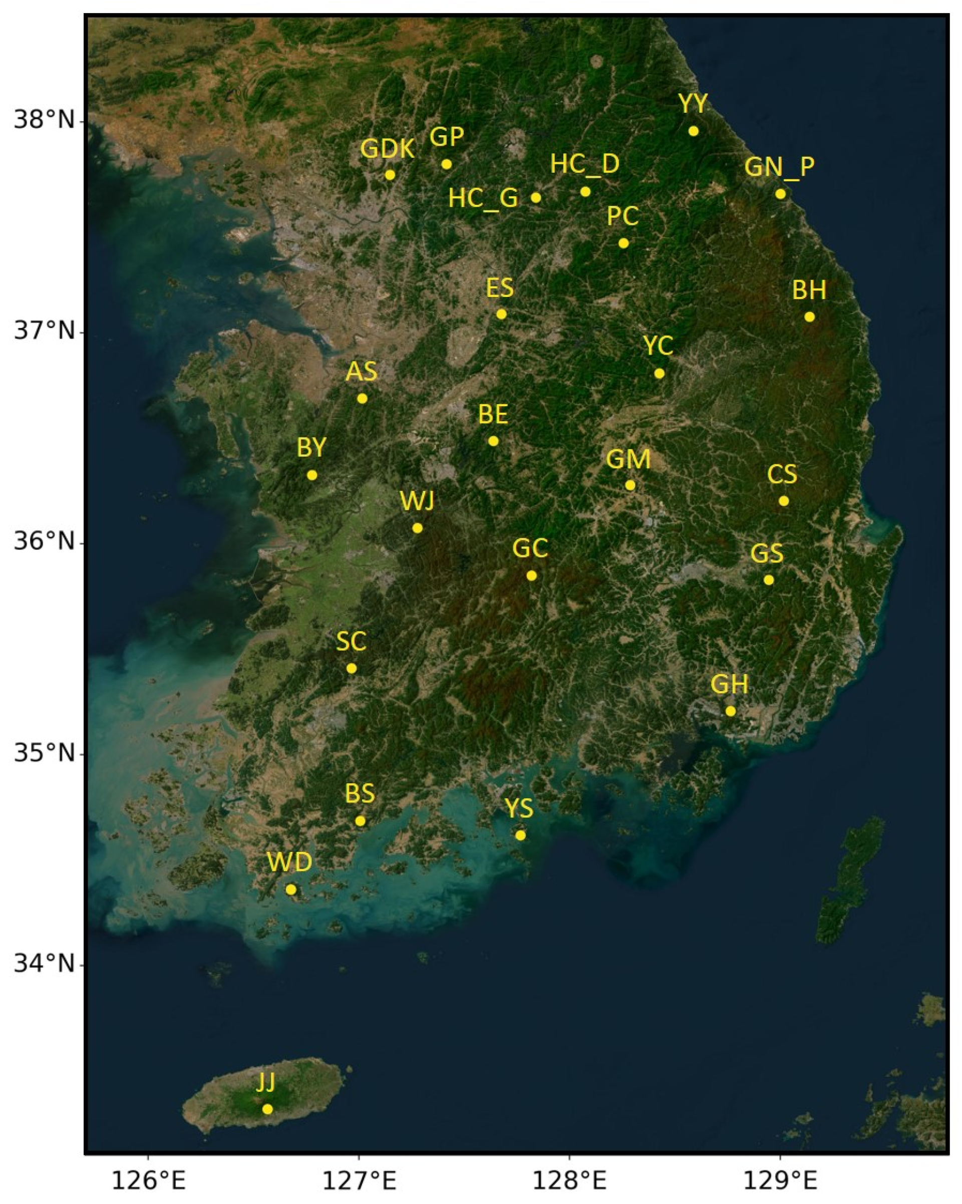
2.1. Study Sites with Ground Observation Network of LAI

This study was conducted at 24 ground observation sites in South Korea, equipped with fisheye lenses for capturing digital hemispherical images (Figure 1 and Table 1). Among the sites, Wando and Jeju installed 5 and 3 fisheye lenses, respectively, and other sites had 1 fisheye lens each (a total of 30 fisheye lenses across South Korea). The sites were strategically selected based on a diversity of forest types and climatic conditions to ensure a comprehensive analysis. Forest types were identified through field surveys and classified into five categories: deciduous broadleaf forests (DBFs), deciduous needleleaf forests (DNFs), evergreen broadleaf forests (EBFs), evergreen needleleaf forests (ENFs), and mixed forests (MFs) (Table 1). Similarly, climate diversity was also considered, categorizing the climates of the sites into six distinct types—Cfa, Cwa, Dfa, Dfb, Dwa, and Dwb—according to the high-resolution Köppen Climate Classification map [29] for the period 1991–2020.
LAI and CI were estimated from digital hemispherical images captured by fisheye lenses within the ground observation network. We analyzed the data recorded in 2023 since most sites were installed in 2023, except for GDK, WD, and JJ. The fisheye lenses have been capturing hemispherical images at one-hour intervals, but there were gaps in the data due to internet connection issues and power supply equipment problems (refer to Table 1). The methodology for estimating LAI and CI followed the automatic framework described in [30], with the view zenith angle specifically constrained to 40 degrees. The CI was calculated according to the hemispheR R library [31,32]. For data quality control under different light conditions, LAI and CI values outside two standard deviations within the moving window of 14 and 7 days were filtered out.
Table 1. Locations of the automatic network for LAI observation, covering 24 sites across South Korea. Only Wando (WD) and Jeju (JJ) are equipped with 5 and 3 fisheye lenses, respectively, while the remaining sites each have 1 fisheye lens installed. The exact dates of data collection are detailed in the last column. The Köppen Climate Classification [29] categorizes our sites into 6 groups: Cfa (Temperate, no dry season, hot summer), Cwa (Temperate, dry winter, hot summer), Dfa (Cold, no dry season, hot summer), Dfb (Cold, no dry season, warm summer), Dwa (Cold, dry winter, hot summer), and Dwb (Cold, dry winter, warm summer). The forest types across our sites were identified as deciduous broadleaf forests (DBFs), deciduous needleleaf forests (DNFs), evergreen broadleaf forests (EBFs), evergreen needleleaf forests (ENFs), and mixed forests (MFs).
Site NameAbbreviationsLongitudeLatitudeKöppen Climate ClassificationForest TypeObservation
Period
AsanAS127.016536.6893DwaMF23.08.27–23.11.24
23.11.29–23.11.30
BoeunBE127.638936.4875DwaDBF23.11.11–23.11.30
BonghwaBH129.139437.0758DfbDBF23.06.18–23.09.30
23.11.07–23.11.30
BoseongBS127.006734.6854CwaDBF23.04.30–23.08.01
23.11.10–23.11.24
23.11.29–23.11.30
BuyeoBY126.778536.3257DwaMF23.08.27–23.11.24
CheongsongCS129.017236.2025DwaMF23.03.11–23.08.02
23.08–03-23.10.12
23.11.08–23.11.24
23.11.29–23.11.30
EumseongES127.676437.0882DwaDBF23.08.02–23.11.24
23.11.29–23.11.30
Gangneung_PGN_P129.001037.6589DfaMF23.06.01–23.07.27
23.08.11–23.08.16
23.11.30
GapyeongGP127.416837.8005DwaDBF23.09.23–23.11.30
GeochangGC127.819235.8495DwaDBF23.02.26–23.10.01
23.11.09–23.11.30
GimhaeGH128.764735.2053CwaDBF23.06.19–23.11.24
23.11.29–23.11.30
GumiGM128.287636.2780DwaMF23.03.12–23.08.05
23.08.25–23.08.27
23.11.09–23.11.15
GwangneungGDK127.148737.7488DwaDBF21.12.17–23.03.24
GyeongsanGS128.945135.8286DwaENF23.03.12–23.08.30
23.11.09–23.11.30
Hongcheon_DHC_D128.074837.6695DwaDBF23.08.08–23.11.24
23.11.29–23.11.30
Hongcheon_GHC_G127.840737.6410DwaDBF23.08.08–23.11.24
23.11.29–23.11.30
JejuJJ1126.567733.3179CfaMF22.08.26–23.07.25
23.09.05–23.11.24
23.11.29–23.11.30
JJ2126.567633.3178CfaMF22.08.26–23.07.25
23.09.05–23.11.24
23.11.29–23.11.30
JJ3126.567533.3178CfaEBF22.08.26–23.07.25
PyeongchangPC128.255937.4258DwbDNF23.06.01–23.07.07
23.07.15–23.07.20
23.07.29–23.08.03
23.09.09–23.09.17
SunchangSC126.966435.4098DfaDBF23.05.27–23.11.24
23.11.29–23.11.30
WandoWD1126.677934.3594CfaEBF22.11.01–23.06.15
23.08.25–23.08.27
23.11.11–23.11.16
WD2126.677634.3594CfaEBF22.11.01–23.06.15
23.08.25–23.08.27
23.11.11–23.11.24
23.11.29–23.11.30
WD3126.677834.3593CfaEBF23.05.01–23.07.02
23.08.25–23.09.04
23.11.11–23.11.24
23.11.29–23.11.30
WD4126.677734.3592CfaEBF22.11.01–23.07.02
23.08.25–23.09.04
23.11.11–23.11.24
23.11.29–23.11.30
WD5126.677934.3593CfaEBF22.11.01–23.05.04
23.11.11–23.11.24
23.11.29–23.11.30
WanjuWJ127.277836.0748DwaDBF23.02.25–23.05.14
23.05.22–23.05.26
23.06.05
23.08.26–23.11.24
23.11.29–23.11.30
YangYangYY128.588837.9569DfbDBF23.09.22–23.11.24
23.11.29–23.11.30
YecheonYC128.425936.8083DwaDBF23.03.13–23.11.24
23.11.29–23.11.30
YeosuYS127.767634.6162CwaMF23.06.04–23.11.24
23.11.29–23.11.30
Figure 1. Study area illustrating the ground observation sites for LAI. Yellow points indicate the site location, and yellow texts denote the abbreviated site name (refer to Table 1).
Forests 15 00665 g001

2.2. DEM

For the topographic correction detailed in Section 2.3, we acquired a digital elevation model (DEM) to calculate terrain slope and aspect. The DEM, which was provided by the National Geographic Information Institute in South Korea and had a 90 m spatial resolution, was downloaded from https://www.vworld.kr. We then calculated the slope and aspect based on this DEM using the toolbox in QGIS version 3.28.15.

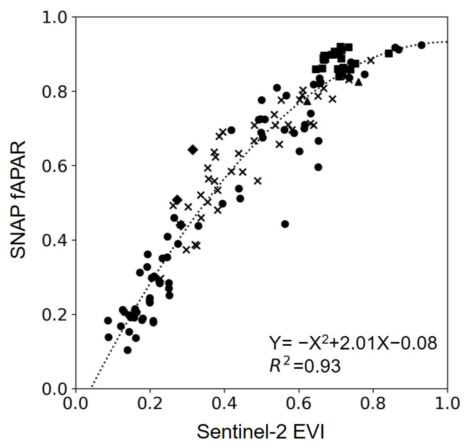
2.3. Sentinel-2 Vegetation Indices

In this study, Sentinel-2 Level 2A (L2A) surface reflectance data from January to November 2023 were used (https://dataspace.copernicus.eu, last accessed in 12 December 2023). To ensure data quality and minimize cloud contamination, Sentinel-2 L2A tiles with a cloud probability exceeding 20% were excluded. In addition, for rigorous quality control, pixels identified as saturated or defective, along with those affected by cloud shadows, medium to high cloud probability, thin cirrus clouds, and snow presence, were filtered out. The collection dates of the Sentinel-2 tiles used in the analysis are provided in Table S1.
Two vegetation indices, NIRv and enhanced vegetation index (EVI), were derived from the surface reflectance data of Sentinel-2 L2A [33,34]. Due to the study sites being located in mountainous areas, the impact of terrain on illumination conditions was often substantial, and thus, topographic effects were corrected to prevent distortion of the vegetation indices [16]. We applied the path length correction (PLC) method, referring to [35]. This method uses a topographic normalization conversion factor ( P ) to adjust the reflectance from a sloped surface ( ρ o r i ) to its horizontal equivalent ( ρ P L C ), as shown in Equation (3).
ρ P L C = P × ρ o r i
P = S Ω s + S ( Ω v ) S t Ω s + S t ( Ω v )
S θ = 1 / c o s θ
S t θ , φ , α , β = 1 c o s θ ( 1 t a n α · c o s ( φ β ) · t a n θ )
The topographic normalization conversion factor (P) normalizes path lengths between horizontal ( S θ ) and sloping surfaces ( S t θ , φ , α , β ), as shown in Equation (4). Here, Ω s and Ω v denote the solar and sensor viewing angles, respectively, with θ and φ representing the zenith and azimuth angles for Ω s and Ω v . The parameters α and β indicate the slope and aspect of the terrain, which were calculated from the DEM. The vegetation indices with topographic correction are labeled as NIRvPLC and EVIPLC, whereas those calculated from original reflectance are denoted as NIRvori and EVIori.

2.4. SNAP LAI and fAPAR

To estimate LAI and fAPAR, Sentinel-2 L2A data at a 20 m spatial resolution were processed through the Sentinel-2 land biophysical processor available in the Sentinel application platform (SNAP) toolbox. The biophysical processor utilizes eight reflectance bands (B3, B4, B5, B6, B7, B8A, B11, and B12) and incorporates viewing zenith, solar zenith, and relative azimuth angles into radiative transfer models, specifically PROSAIL and a neural network algorithm [36].

2.5. Tower-Based Multispectral Reflectance

To compare with satellite-based data, tower-based vegetation indices, including NIRv and EVI, were calculated. Surface reflectance data were collected using LED-based multispectral sensors developed by SolDan Inc. The SD-600 model, equipped with the AS7343 sensor produced by ams-OSRAM AG (https://ams-osram.com/products/sensors/ambient-light-color-spectral-proximity-sensors/ams-as7343-spectral-sensor, accessed on 12 January 2024), has operated at eight sites since 2023. Among the eight sites, the Wando (from 15 April 2023) and Jeju (from 25 June 2023) sites overlapped with the ground observation network of LAI. In five spectral bands—blue, green, red, red edge, and near-infrared—the spectral wavelengths of SD-600 closely match those of Sentinel-2 (Table 2).

3. Methods

3.1. fesc Calculation

fesc can be approximated by dividing NIRv by fAPAR, as demonstrated in Equation (1). For Sentinel-2 data, LAI and fAPAR were derived via the SNAP toolbox, permitting the calculation of fesc by Equation (1). To evaluate the effect of topographic correction on fesc, we calculated NIRv values with and without topographic correction for the satellite-based fesc.
Directly measuring fAPAR with in situ multispectral sensors often presents practical difficulties. As previous studies have shown that EVI has a high correlation with fAPAR [37,38], we fitted a regression line between EVI and fAPAR obtained from Sentinel-2 data (Figure 2). We then estimated fAPAR by applying a regression equation to the field-based EVI, calculated with the same EVI equation used for Sentinel-2 data. The estimated field-based fAPAR was used to calculate the field-based fesc with the field-based NIRv.

3.2. Comparison between Canopy Structure and fesc

The fesc is theoretically expected to show a high correlation with canopy structure, given the significant impact of canopy structure on photosynthetic efficiency and energy exchange processes within plant canopies. To grasp whether spectral invariant theory-based fesc (Equation (1)) has a high correlation with canopy structure, we analyzed the correlation between fesc and various indicators—LAI, CI, and the combined metric of LAI and CI (i.e., LAI×CI). To ensure consistency between satellite-based and ground-based data, fesc estimates from Sentinel-2 and ground observation data, along with available canopy structural indicators, were utilized in this analysis. The correlation analysis was conducted by calculating the slope, intercept, and coefficient of determination (R2) on scatter plots with canopy structural indicators on the X-axis and fesc on the Y-axis. Significance was determined via p-values using a one-tailed t-test. We also further analyzed NIRv to evaluate the relative influence of canopy structure in Equation (1).

4. Results

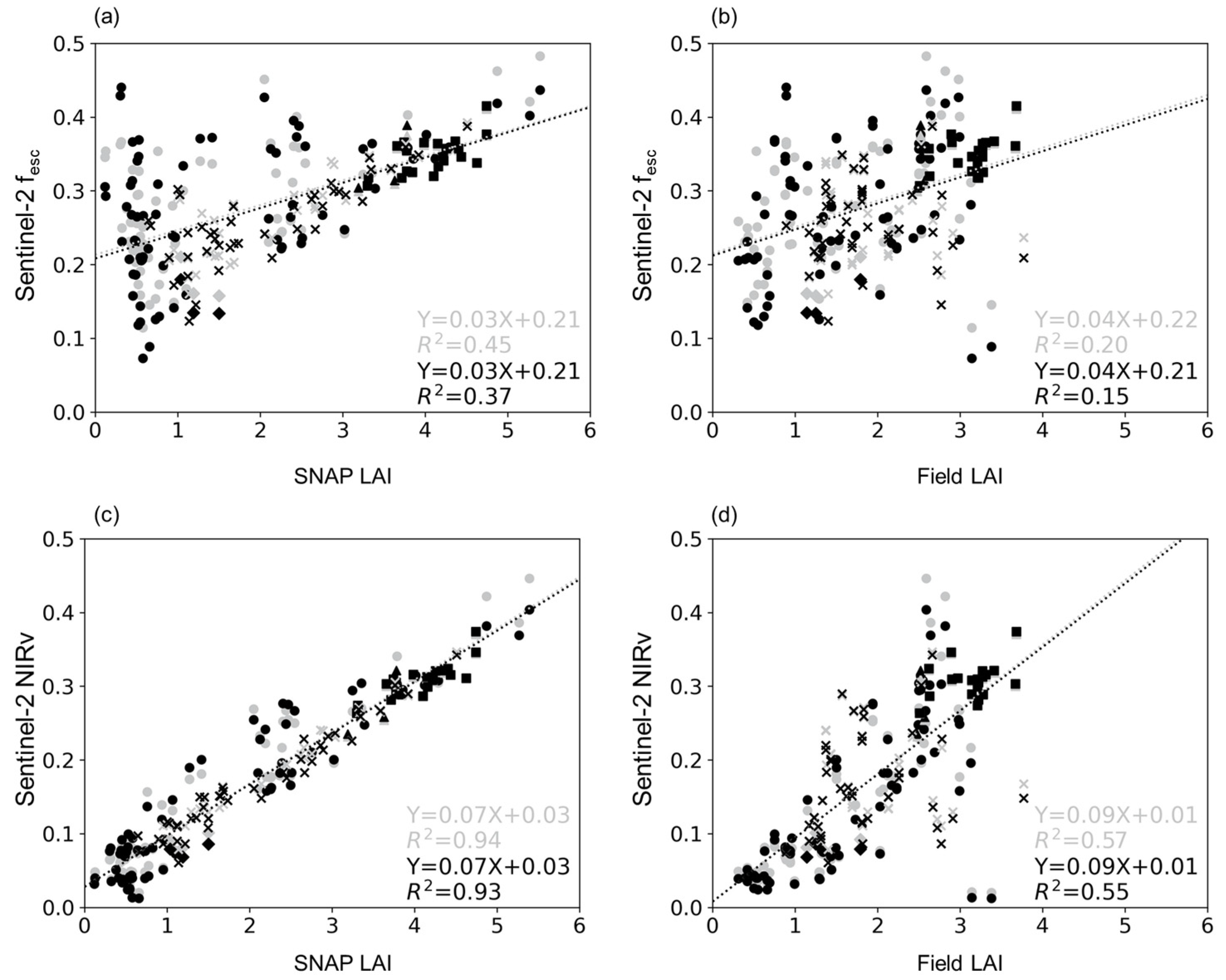
4.1. Relationship between LAI and fesc

Comparisons between Sentinel-based fesc and SNAP LAI, as well as field-based LAI, are presented in Figure 3a,b. Overall, the correlations were highly significant (p-value < 0.001), and topographic correction resulted in a decrease in R2 rather than the original data, while the regression trends remained similar before and after correction. The relationship between Sentinel-based fesc and the LAIs showed similar slopes between satellite-based and field-based data, ranging from 0.03 to 0.04, yet R2 markedly decreased to 0.15 for field-based LAI, compared to 0.37 for the satellite-based one. When comparing among forest types (a,b in Tables S2 and S3), excluding needleleaf forests with a small sample size (n < 4), broadleaf forests exhibited slopes and R2 values similar to the overall trend. MF had regression slopes of approximately 0.04 for Sentinel-based fesc against Sentinel-based LAI, similar to those observed in other forest types. However, the regression slopes of Sentinel-based fesc, when compared with field-based LAI, varied from 0.001 to 0.007, with a significant decrease in R2 to a range between 0.00 and 0.01.
Sentinel-based NIRv generally had a strong correlation with LAI data (R2 > 0.55), as shown in Figure 3c,d. Notably, the correlation between Sentinel-based NIRv and SNAP LAI was particularly strong, with R2 values between 0.93 and 0.94. Their correlation remained strong across forest types (c,d in Tables S2 and S3), with R2 values exceeding 0.68, except for ENF. However, when comparing Sentinel-based NIRv with field-based LAI, all forest types other than DBF, which had R2 values between 0.53 and 0.55, showed R2 values below 0.2, with the regression slopes significantly reduced to around 0.02.
Comparing the regression lines from Figure 3a,b with those from Figure 3c,d revealed that the slopes for LAI and NIRv were approximately twice that of the slopes for LAI and fesc. This pattern of slopes is also evident when using field-based data from WD and JJ, as shown in Figure 4. In WD, classified as EBF, the correlation between LAI and fesc was low at 0.05, and the correlation between LAI and NIRv was also low at 0.08. For the JJ site, characterized as MF, while the slopes for LAI and fesc, as well as NIRv, were low (0.02–0.03), the R2 is relatively high at approximately 0.5. This indicates a stronger correlation for field-based LAI when compared with field-based fesc or field-based NIRv rather than satellite-based ones.

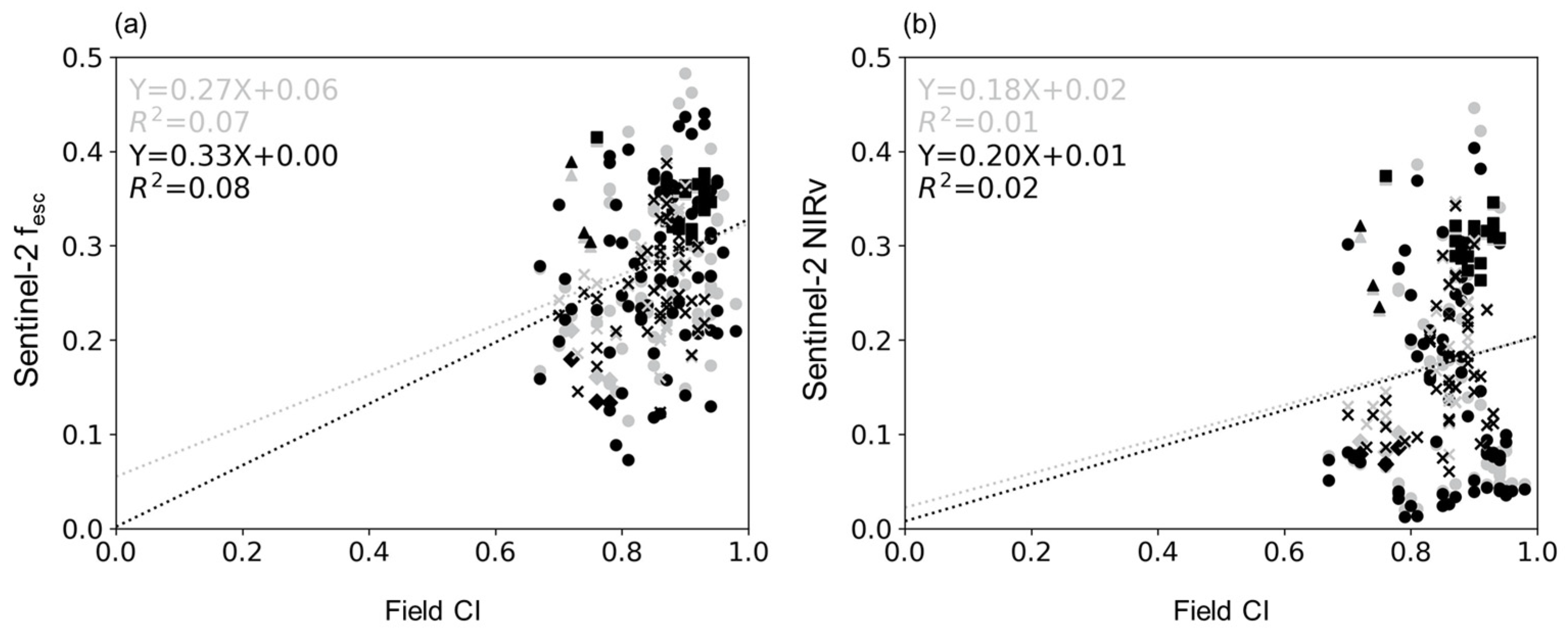
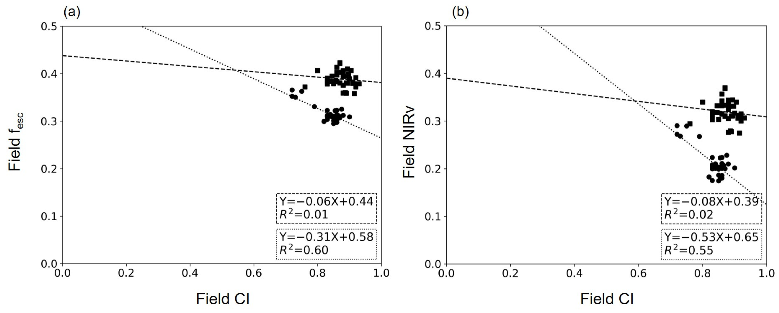
4.2. Relationship between CI and fesc

The comparisons between Sentinel-based fesc and NIRv with field-based CI are illustrated in Figure 5, which are all statistically significant (refer to Tables S4 and S5). In contrast to LAI, CI had a low correlation (R2 less than 0.1) with both fesc and NIRv. This suggests that CI, a measure of aggregation or randomness, has little association with fesc or NIRv. This result was consistent with [39], which demonstrated that horizontal heterogeneity had a stronger effect on SIF than vertical heterogeneity. When compared by forest type, fesc and NIRv only in EBF showed R2 values of approximately 0.15 and 0.11, respectively, while other forest types exhibited R2 values less than 0.1. As mentioned in Section 4.1, while LAI had a relatively higher correlation with NIRv than with fesc, CI showed slightly higher R2 values with fesc than with NIRv.
Field-based comparisons from WD and JJ (Figure 6) revealed different trends compared to Sentinel-based fesc and NIRv. While the regression slopes between field-based CI and Sentinel-based fesc and NIRv were positive, Figure 6 showed negative slopes for both WD and JJ between field-based fesc and NIRv. This pattern suggests that the CI response to fesc and NIRv varies by forest type, with both showing negative regression slopes when comparing Sentinel-based fesc and NIRv with field-based CI (Tables S4 and S5). Therefore, the relationship between CI and both fesc and NIRv is inferred to vary depending on the forest type.

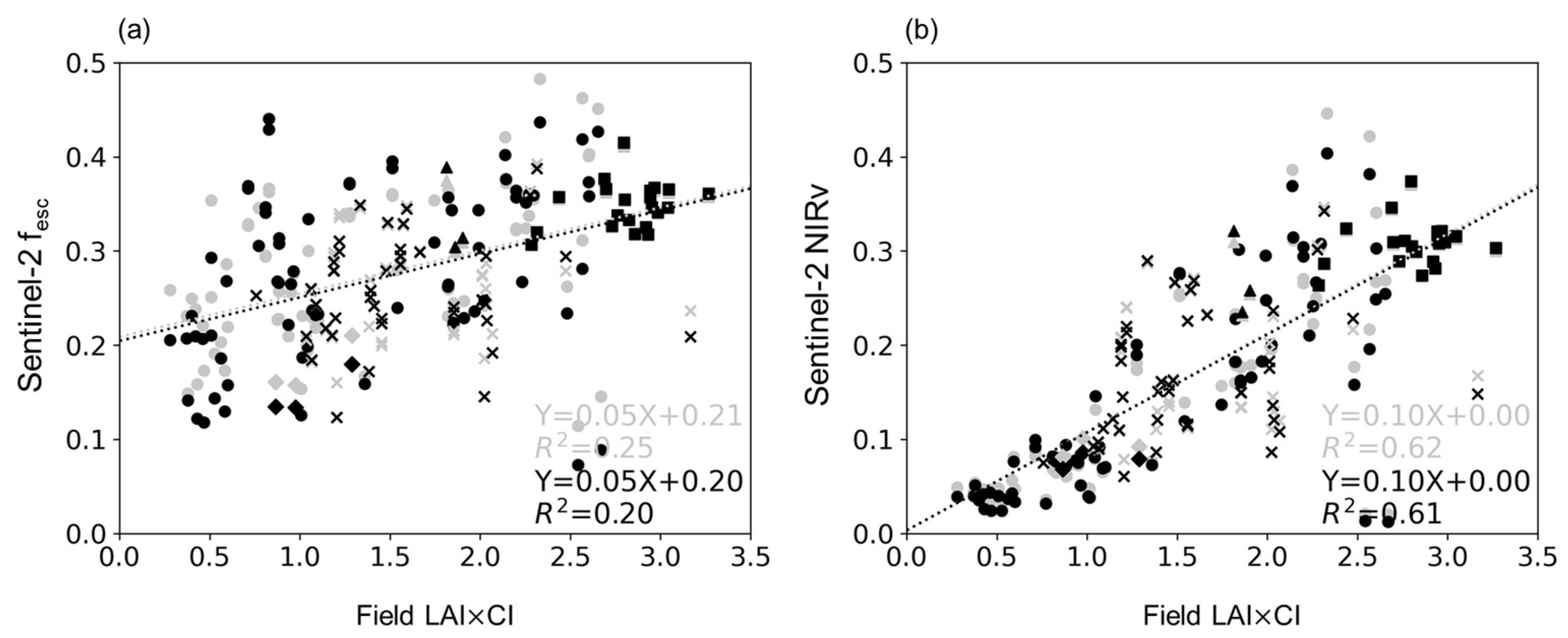
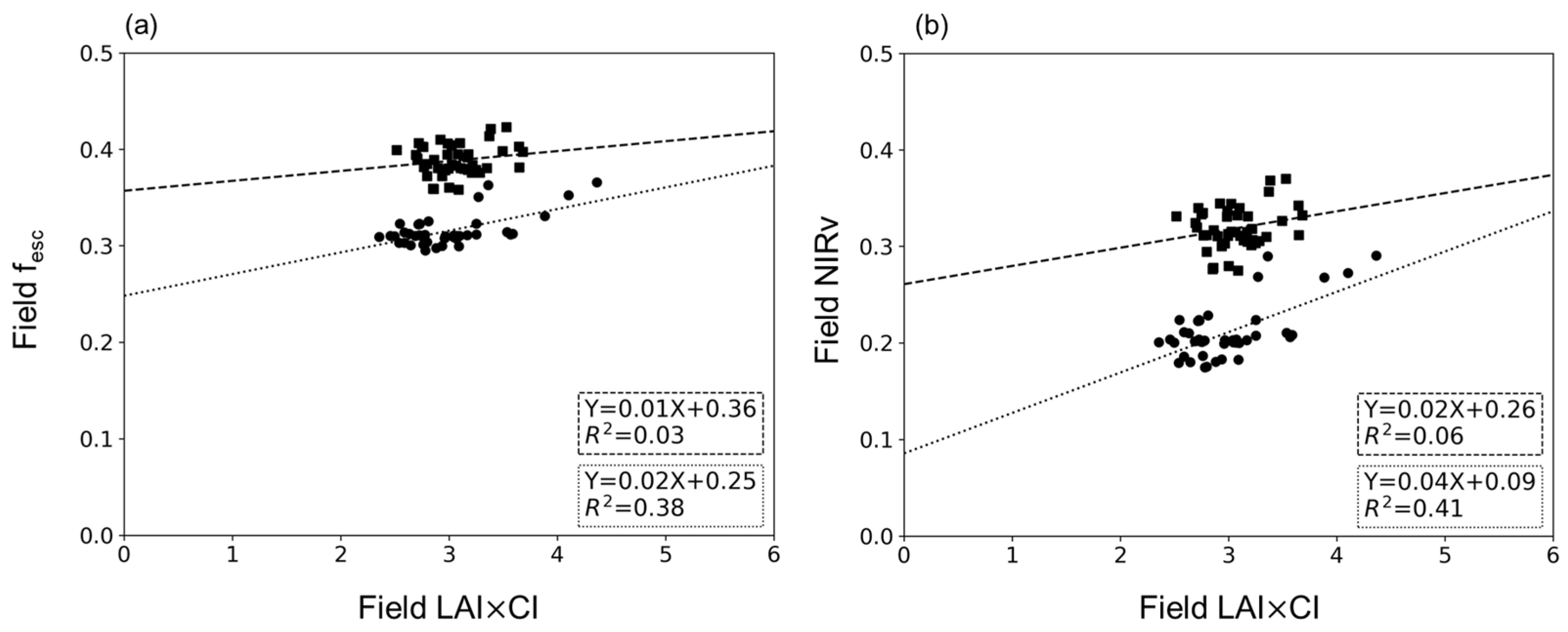
4.3. Relationship between LAI×CI and fesc

In the comparison of field-based LAI×CI with Sentinel-based fesc and NIRv, as shown in Figure 7, we found that multiplying LAI by CI did not improve their correlation with fesc and NIRv. Specifically, while LAI×CI had higher correlations with fesc and NIRv than CI (discussed in Section 4.2), they did not reach the correlation levels observed with LAI (noted in Section 4.1). In a similar pattern to LAI, the coefficient of determination (R2) for the comparison of field-based LAI×CI with Sentinel-based fesc was approximately 0.2, whereas it increased to about 0.6 when comparing LAI×CI with Sentinel-based NIRv. Across most forest types, we observed weak yet positive correlations between CI and both fesc and NIRv (Tables S6 and S7). However, these correlations were weaker than those seen with LAI alone, as detailed in Section 4.1. Additionally, Figure 8, which presents field-based data, reinforces this trend, indicating that NIRv generally has a stronger correlation (higher R2 values) with LAI×CI than fesc does.

5. Discussion

The fesc, representing the ratio between the observed SIF on top of the canopy and the canopy-level SIF, plays a crucial role in translating satellite-observed SIF into the canopy level. Theoretically, fesc is intimately linked with canopy structure. For instance, within the GPP-SIF760 relationship, changes in canopy structure emerged as a more influential driving factor than either chlorophyll a and b or the maximum carboxylation rate at 25 °C [39]. However, fesc calculations still have large deviations according to the assumptions that simplify the equations based on the spectral invariant theory. In [2], the fesc values were calculated using the method described in [27], N I R / i 0 ω N , with those obtained using the ratio of NIRv to fAPAR being compared with the SCOPE simulation-based fesc. The former method includes total NIR, which includes the soil signal, whereas the latter uses NIRv. In comparison to SCOPE simulations, the NIRv-based fesc closely matched a 1:1 ratio, achieving an R2 of 0.91, while the method described in [27] resulted in overestimation, with an R2 value of 0.11. The performance of fesc estimates varied depending on the input data for the ratio of NIRv to fAPAR. The estimated fesc in [40] was underestimated compared to SCOPE simulations, with R2 around 0.7. The SIF was retrieved using field-based hyperspectral data, and fAPAR was estimated using a digital camera with the reference panel for the green component. Although fesc values were calculated with different equations and input data in the above studies and validated against SCOPE simulations, determining a direct physical correlation with canopy structure requires further exploration.
As LAI increases, the total SIF also tends to increase [27], suggesting a strong correlation between LAI and the fesc. However, neither our study nor the findings in [41] demonstrated a significant impact of LAI on fesc in the NIR region. The weak relationships between fesc and LAI can be attributed to the absence of noticeable phenological changes when fesc estimates are presented as time series data, as seen in both Figure 9 and [39]. Conceptually, it is expected that fesc values would fluctuate with changes in canopy structure. The absence of phenological changes in fesc is expected to result from the offset of canopy structure effects during the calculation. Such offset is thought to occur by dividing NIRv by variables closely related to canopy structure, such as canopy interceptance or fAPAR, which approximates canopy interceptance [42]. Nonetheless, direct interpretation between canopy structure and fesc remains a challenge in remote sensing and modeling fields [43].
In addition to LAI and CI, factors such as leaf angle distribution (LAD) and soil reflectance can also influence fesc. LAD, a critical parameter affecting the angular distribution of reflected photons, significantly impacts the scattering and escape probability, thereby influencing directional SIF. In particular, the differences in LAD within dense canopies lead to minor differences in total SIF [44]. Similarly, [45] demonstrated a close relationship between recollision probability and LAI, but the relationship varied with canopy shoot even under the same LAI. Furthermore, soil reflectance plays a role in the estimation of the ratio of NIRv to fAPAR. [40] applied a Gaussian process regression algorithm for correcting soil reflectance, resulting in a significant enhancement in the accuracy of fesc when validated with SCOPE simulations; R2 values improved from 0.86 to 0.95, and root mean squared error decreased from 0.1 to 0.01. In this study, the canopy density of most sites was very high, so the influence of slight LAD fluctuations and soil reflectance on the analysis results is expected to be minimal. However, the presence of diverse tree species and phenological-driven changes in canopy density make it necessary to consider such factors in future research.
The method for estimating fesc based on the ratio of NIRv to fAPAR, as introduced in [2], is readily adaptable to satellite data. This study conducted terrain correction on Sentinel-2-based NIRv to mitigate terrain effects yet observed no notable improvement in performance. Furthermore, the difficulty in obtaining satellite imagery during growing seasons because of cloud contamination may result in analysis bias. To accurately assess how satellite-derived fesc estimates correlate with canopy structure, accurate NIRv measurements across different periods are essential. Consequently, nadir BRDF-adjusted reflectance data [46,47] in the NIR and red bands are deemed necessary. Moreover, enhancing the accuracy of satellite-based fAPAR is critical. A comparison of Sentinel-2-based fAPAR with field observations revealed variations in R2 from 0.22 to 0.64 across different sites, with an absolute discrepancy of up to 25% [48], significantly affecting the performance of the NIRv to fAPAR ratio. The analysis and estimation of fesc must also consider the potential underestimation of satellite-derived LAI and CI [25], in addition to considering the uncertainties of NIRv and fAPAR. For example, the LAI model within the SNAP toolbox has been reported to overestimate in areas of dense vegetation [49]. Therefore, in order to quantify the uncertainty and improve performance on satellite-based fesc, it is considered useful to introduce an algorithm to directly estimate fesc using canopy structural parameters.

6. Conclusions

This study elucidates the quantitative relationship between canopy structure and canopy escape ratio (fesc), the ratio of NIRv to fAPAR. We compared the fesc with canopy structure data (e.g., LAI and CI) through both satellite-based and in situ observations to find out whether the findings are consistent between data. Considering the spatial footprint of the field observations, we used Sentinel-2 imagery for comparison. Since the ratio of NIRv to fAPAR is a simplified equation based on spectral invariant theory, fesc was expected to be highly correlated with LAI and CI, which affect light transmittance, absorption, and reflection within the canopy. According to our results, LAI had the highest R2 of 0.37 and 0.15 for SNAP LAI and field-based LAI, respectively, but the relationship between CI and fesc showed little correlation, with an R2 value of less than 0.1. Such correlations between canopy structure and fesc differed in accordance with forest types. Our results also showed that the canopy structures are more strongly correlated with NIRv than fesc. Notably, the phenological pattern of fesc was almost constant when comparing fesc and LAI in a time series based on field observation. We speculate that the correlation between canopy structure and fesc decreased in the ratio of NIRv to fAPAR due to the high correlation between LAI and fAPAR. Despite advancements in estimating fesc using NIRv to fAPAR, further enhancements are necessary to address significant uncertainties, including those associated with equation assumptions, leaf angle distribution, soil reflectance, and the estimation of LAI and fAPAR derived from satellites. Our results help to better understand the current estimation of canopy escape probability based on the ratio of NIRv to fAPAR and provide guidance for improving the equation in future research. In addition, our research could substantially contribute to bridging a crucial gap in understanding how canopy structures affect light dynamics across different biomes and enhance global vegetation monitoring efforts.

Supplementary Materials

The following supporting information can be downloaded at: https://www.mdpi.com/article/10.3390/f15040665/s1, Table S1: Sentinel-2 image acquisition dates are shown in gray; Table S2: Relationship between LAI and Sentinel-based fesc and NIRv across different forest types without topographic correction; Table S3: Relationship between LAI and Sentinel-based fesc and NIRv on different forest types with topographic correction; Table S4: Relationship between CI and Sentinel-based fesc and NIRv on different forest types without topographic correction; Table S5: Relationship between CI and Sentinel-based fesc and NIRv on different forest types with topographic correction; Table S6: Relationship between LAI × CI and Sentinel-based fesc and NIRv on different forest types without topographic correction; Table S7: Relationship between LAI × CI and Sentinel-based fesc and NIRv on different forest types with topographic correction.

Author Contributions

Conceptualization, J.L. (Junghee Lee); methodology, J.L. (Junghee Lee); formal analysis, J.L. (Junghee Lee); resources, J.L. (Junghee Lee) and J.L. (Joongbin Lim); writing—original draft preparation, J.L. (Junghee Lee); writing—review and editing, J.I.; visualization, J.L. (Junghee Lee); supervision, J.L. (Joongbin Lim) and K.K.; project administration, K.K.; funding acquisition, K.K. All authors have read and agreed to the published version of the manuscript.

Funding

This research was supported by the development of agricultural and forestry satellite convergence products of analysis-ready data (FM0103-2021-01-2024) and continuous forest disaster surveillance and ecosystem monitoring (FM0103-2021-02-2023 and FM0103-2021-02-2024) from the National Institute of Forest Science of the Korea Forest Service, Republic of Korea.

Data Availability Statement

Data are available from the authors on request.

Conflicts of Interest

The authors declare no conflicts of interest.

References

  1. Badgley, G.; Anderegg, L.D.L.; Berry, J.A.; Field, C.B. Terrestrial Gross Primary Production: Using NIRV to Scale from Site to Globe. Glob. Change Biol. 2019, 25, 3731–3740. [Google Scholar] [CrossRef]
  2. Zeng, Y.; Badgley, G.; Dechant, B.; Ryu, Y.; Chen, M.; Berry, J.A. A Practical Approach for Estimating the Escape Ratio of Near-Infrared Solar-Induced Chlorophyll Fluorescence. Remote Sens. Environ. 2019, 232, 111209. [Google Scholar] [CrossRef]
  3. Zhu, W.; Xie, Z.; Zhao, C.; Zheng, Z.; Qiao, K.; Peng, D.; Fu, Y.H. Remote Sensing of Terrestrial Gross Primary Productivity: A Review of Advances in Theoretical Foundation, Key Parameters and Methods. GISci. Remote Sens. 2024, 61, 2318846. [Google Scholar] [CrossRef]
  4. Wang, S.; Zhang, Y.; Ju, W.; Qiu, B.; Zhang, Z. Tracking the Seasonal and Inter-Annual Variations of Global Gross Primary Production during Last Four Decades Using Satellite near-Infrared Reflectance Data. Sci. Total Environ. 2021, 755, 142569. [Google Scholar] [CrossRef] [PubMed]
  5. Wu, G.; Guan, K.; Jiang, C.; Peng, B.; Kimm, H.; Chen, M.; Yang, X.; Wang, S.; Suyker, A.E.; Bernacchi, C.J.; et al. Radiance-Based NIRv as a Proxy for GPP of Corn and Soybean. Environ. Res. Lett. 2020, 15, 34009. [Google Scholar] [CrossRef]
  6. Dechant, B.; Ryu, Y.; Badgley, G.; Köhler, P.; Rascher, U.; Migliavacca, M.; Zhang, Y.; Tagliabue, G.; Guan, K.; Rossini, M.; et al. NIRVP: A Robust Structural Proxy for Sun-Induced Chlorophyll Fluorescence and Photosynthesis across Scales. Remote Sens. Environ. 2022, 268, 112763. [Google Scholar] [CrossRef]
  7. Jin, J.; Hou, W.; Ma, X.; Wang, H.; Xie, Q.; Wang, W.; Zhu, Q.; Fang, X.; Zhou, F.; Liu, Y.; et al. Improved Estimation of Gross Primary Production with NIRvP by Incorporating a Phenophase Scheme for Temperate Deciduous Forest Ecosystems. For. Ecol. Manage 2024, 556, 121742. [Google Scholar] [CrossRef]
  8. Huang, X.; Xiao, J.; Ma, M. Evaluating the Performance of Satellite-Derived Vegetation Indices for Estimating Gross Primary Productivity Using FLUXNET Observations across the Globe. Remote Sens. 2019, 11, 1823. [Google Scholar] [CrossRef]
  9. Yang, R.; Wang, J.; Zeng, N.; Sitch, S.; Tang, W.; McGrath, M.J.; Cai, Q.; Liu, D.; Lombardozzi, D.; Tian, H.; et al. Divergent Historical GPP Trends among State-of-the-Art Multi-Model Simulations and Satellite-Based Products. Earth Syst. Dyn. 2022, 13, 833–849. [Google Scholar] [CrossRef]
  10. McMahon, D.E.; Jackson, R.B. Management Intensification Maintains Wood Production over Multiple Harvests in Tropical Eucalyptus Plantations. Ecol. Appl. 2019, 29, e01879. [Google Scholar] [CrossRef]
  11. Tang, L.; Zhang, S.; Zhang, J.; Liu, Y.; Bai, Y. Estimating Evapotranspiration Based on the Satellite-Retrieved near-Infrared Reflectance of Vegetation (NIRv) over Croplands. GISci. Remote Sens. 2021, 58, 889–913. [Google Scholar] [CrossRef]
  12. Merrick, T.; Pau, S.; Detto, M.; Broadbent, E.N.; Bohlman, S.A.; Still, C.J.; Almeyda Zambrano, A.M. Unveiling Spatial and Temporal Heterogeneity of a Tropical Forest Canopy Using High-Resolution NIRv, FCVI, and NIRvrad from UAS Observations. Biogeosciences 2021, 18, 6077–6091. [Google Scholar] [CrossRef]
  13. Baldocchi, D.D.; Ryu, Y.; Dechant, B.; Eichelmann, E.; Hemes, K.; Ma, S.; Sanchez, C.R.; Shortt, R.; Szutu, D.; Valach, A.; et al. Outgoing Near-Infrared Radiation From Vegetation Scales With Canopy Photosynthesis Across a Spectrum of Function, Structure, Physiological Capacity, and Weather. J. Geophys. Res. Biogeosci. 2020, 125, e2019JG005534. [Google Scholar] [CrossRef]
  14. Yang, Y.; Chen, R.; Yin, G.; Wang, C.; Liu, G.; Verger, A.; Descals, A.; Filella, I.; Peñuelas, J. Divergent Performances of Vegetation Indices in Extracting Photosynthetic Phenology for Northern Deciduous Broadleaf Forests. IEEE Geosci. Remote Sens. Lett. 2022, 19, 1–5. [Google Scholar] [CrossRef]
  15. Ersi, C.; Bayaer, T.; Bao, Y.; Bao, Y.; Yong, M.; Lai, Q.; Zhang, X.; Zhang, Y. Comparison of Phenological Parameters Extracted from SIF, NDVI and NIRv Data on the Mongolian Plateau. Remote Sens. 2022, 15, 187. [Google Scholar] [CrossRef]
  16. Chen, R.; Yin, G.; Liu, G.; Yang, Y.; Wang, C.; Xie, Q.; Zhao, W.; Verger, A. Correction of Illumination Effects on Seasonal Divergent NIRv Photosynthetic Phenology. Agric. For. Meteorol. 2023, 339, 109542. [Google Scholar] [CrossRef]
  17. Zhang, J.; Xiao, J.; Tong, X.; Zhang, J.; Meng, P.; Li, J.; Liu, P.; Yu, P. NIRv and SIF Better Estimate Phenology than NDVI and EVI: Effects of Spring and Autumn Phenology on Ecosystem Production of Planted Forests. Agric. For. Meteorol. 2022, 315, 108819. [Google Scholar] [CrossRef]
  18. Qiu, R.; Li, X.; Han, G.; Xiao, J.; Ma, X.; Gong, W. Monitoring Drought Impacts on Crop Productivity of the US Midwest with Solar-Induced Fluorescence: GOSIF Outperforms GOME-2 SIF and MODIS NDVI, EVI, and NIRv. Agric. For. Meteorol. 2022, 323, 109038. [Google Scholar] [CrossRef]
  19. Zeng, Y.; Chen, M.; Hao, D.; Damm, A.; Badgley, G.; Rascher, U.; Johnson, J.E.; Dechant, B.; Siegmann, B.; Ryu, Y.; et al. Combining Near-Infrared Radiance of Vegetation and Fluorescence Spectroscopy to Detect Effects of Abiotic Changes and Stresses. Remote Sens. Environ. 2022, 270, 112856. [Google Scholar] [CrossRef]
  20. Gu, H.; Yin, G.; Yang, Y.; Verger, A.; Descals, A.; Filella, I.; Zeng, Y.; Hao, D.; Xie, Q.; Li, X.; et al. Satellite-Detected Contrasting Responses of Canopy Structure and Leaf Physiology to Drought. IEEE J. Sel. Top. Appl. Earth Obs. Remote Sens. 2023, 16, 2427–2436. [Google Scholar] [CrossRef]
  21. Chen, J.; Liu, X.; Du, S.; Ma, Y.; Liu, L. Effects of Drought on the Relationship between Photosynthesis and Chlorophyll Fluorescence for Maize. IEEE J. Sel. Top. Appl. Earth Obs. Remote Sens. 2021, 14, 11148–11161. [Google Scholar] [CrossRef]
  22. Sakai, Y.; Kobayashi, H.; Kato, T. FLiES-SIF Version 1.0: Three-Dimensional Radiative Transfer Model for Estimating Solar Induced Fluorescence. Geosci. Model Dev. 2020, 13, 4041–4066. [Google Scholar] [CrossRef]
  23. Magney, T.S.; Barnes, M.L.; Yang, X. On the Covariation of Chlorophyll Fluorescence and Photosynthesis across Scales. Geophys. Res. Lett. 2020, 47, e2020GL091098. [Google Scholar] [CrossRef]
  24. Maguire, A.J.; Eitel, J.U.H.; Magney, T.S.; Frankenberg, C.; Köhler, P.; Orcutt, E.L.; Parazoo, N.C.; Pavlick, R.; Pierrat, Z.A. Spatial Covariation between Solar-Induced Fluorescence and Vegetation Indices from Arctic-Boreal Landscapes. Environ. Res. Lett. 2021, 16, 95002. [Google Scholar] [CrossRef]
  25. Liu, W.; Luo, S.; Lu, X.; Atherton, J.; Gastellu-Etchegorry, J.-P. Simulation-Based Evaluation of the Estimation Methods of Far-Red Solar-Induced Chlorophyll Fluorescence Escape Probability in Discontinuous Forest Canopies. Remote Sens. 2020, 12, 3962. [Google Scholar] [CrossRef]
  26. Liu, X.; Guanter, L.; Liu, L.; Damm, A.; Malenovský, Z.; Rascher, U.; Peng, D.; Du, S.; Gastellu-Etchegorry, J.-P. Downscaling of Solar-Induced Chlorophyll Fluorescence from Canopy Level to Photosystem Level Using a Random Forest Model. Remote Sens. Environ. 2019, 231, 110772. [Google Scholar] [CrossRef]
  27. Yang, P.; van der Tol, C. Linking Canopy Scattering of Far-Red Sun-Induced Chlorophyll Fluorescence with Reflectance. Remote Sens. Environ. 2018, 209, 456–467. [Google Scholar] [CrossRef]
  28. Filella, I.; Descals, A.; Balzarolo, M.; Yin, G.; Verger, A.; Fang, H.; Peñuelas, J. Photosynthetically Active Radiation and Foliage Clumping Improve Satellite-Based NIRv Estimates of Gross Primary Production. Remote Sens. 2023, 15, 2207. [Google Scholar] [CrossRef]
  29. Lee, J.; Cha, S.; Lim, J.; Chun, J.; Jang, K. Practical LAI Estimation with DHP Images in Complex Forest Structure with Rugged Terrain. Forests 2023, 14, 2047. [Google Scholar] [CrossRef]
  30. Chianucci, F.; Macek, M. HemispheR: An R Package for Fisheye Canopy Image Analysis. Agric. For. Meteorol. 2023, 336, 109470. [Google Scholar] [CrossRef]
  31. Chianucci, F.; Zou, J.; Leng, P.; Zhuang, Y.; Ferrara, C. A New Method to Estimate Clumping Index Integrating Gap Fraction Averaging with the Analysis of Gap Size Distribution. Can. J. For. Res. 2019, 49, 471–479. [Google Scholar] [CrossRef]
  32. Beck, H.E.; McVicar, T.R.; Vergopolan, N.; Berg, A.; Lutsko, N.J.; Dufour, A.; Zeng, Z.; Jiang, X.; van Dijk, A.I.J.M.; Miralles, D.G. High-Resolution (1 Km) Köppen-Geiger Maps for 1901–2099 Based on Constrained CMIP6 Projections. Sci. Data 2023, 10, 724. [Google Scholar] [CrossRef] [PubMed]
  33. Badgley, G.; Field, C.B.; Berry, J.A. Canopy Near-Infrared Reflectance and Terrestrial Photosynthesis. Sci. Adv. 2017, 3, e1602244. [Google Scholar] [CrossRef] [PubMed]
  34. Zhen, Z.; Chen, S.; Yin, T.; Gastellu-Etchegorry, J.-P. Globally Quantitative Analysis of the Impact of Atmosphere and Spectral Response Function on 2-Band Enhanced Vegetation Index (EVI2) over Sentinel-2 and Landsat-8. ISPRS J. Photogramm. Remote Sens. 2023, 205, 206–226. [Google Scholar] [CrossRef]
  35. Chen, R.; Yin, G.; Zhao, W.; Xu, B.; Zeng, Y.; Liu, G.; Verger, A. TCNIRv: Topographically Corrected Near-Infrared Reflectance of Vegetation for Tracking Gross Primary Production Over Mountainous Areas. IEEE Trans. Geosci. Remote Sens. 2022, 60, 1–10. [Google Scholar] [CrossRef]
  36. Weiss, M.; Baret, F.; Jay, S. S2ToolBox Level 2 Products: LAI, FAPAR, FCOVER; Research for Agriculture, Food and Environment (INRAE): Avignon, France, 2016. [Google Scholar]
  37. Ma, X.; Huete, A.; Yu, Q.; Restrepo-Coupe, N.; Beringer, J.; Hutley, L.B.; Kanniah, K.D.; Cleverly, J.; Eamus, D. Parameterization of an Ecosystem Light-Use-Efficiency Model for Predicting Savanna GPP Using MODIS EVI. Remote Sens. Environ. 2014, 154, 253–271. [Google Scholar] [CrossRef]
  38. Liang, S.; Ma, W.; Sui, X.; Wang, M.; Li, H. An Assessment of Relations between Vegetation Green FPAR and Vegetation Indices through a Radiative Transfer Model. Plants 2023, 12, 1927. [Google Scholar] [CrossRef] [PubMed]
  39. Regaieg, O.; Yin, T.; Malenovský, Z.; Cook, B.D.; Morton, D.C.; Gastellu-Etchegorry, J.P. Assessing Impacts of Canopy 3D Structure on Chlorophyll Fluorescence Radiance and Radiative Budget of Deciduous Forest Stands Using DART. Remote Sens. Environ. 2021, 265, 112673. [Google Scholar] [CrossRef]
  40. Qi, M.; Liu, X.; Du, S.; Guan, L.; Chen, R.; Liu, L. Improving the Estimation of Canopy Fluorescence Escape Probability in the Near-Infrared Band by Accounting for Soil Reflectance. Remote Sens. 2023, 15, 4361. [Google Scholar] [CrossRef]
  41. Lu, X.; Liu, Z.; Zhao, F.; Tang, J. Comparison of Total Emitted Solar-Induced Chlorophyll Fluorescence (SIF) and Top-of-Canopy (TOC) SIF in Estimating Photosynthesis. Remote Sens. Environ. 2020, 251, 112083. [Google Scholar] [CrossRef]
  42. Brown, L.A.; Meier, C.; Morris, H.; Pastor-Guzman, J.; Bai, G.; Lerebourg, C.; Gobron, N.; Lanconelli, C.; Clerici, M.; Dash, J. Evaluation of Global Leaf Area Index and Fraction of Absorbed Photosynthetically Active Radiation Products over North America Using Copernicus Ground Based Observations for Validation Data. Remote Sens. Environ. 2020, 247, 111935. [Google Scholar] [CrossRef]
  43. Huang, D.; Knyazikhin, Y.; Dickinson, R.E.; Rautiainen, M.; Stenberg, P.; Disney, M.; Lewis, P.; Cescatti, A.; Tian, Y.; Verhoef, W.; et al. Canopy Spectral Invariants for Remote Sensing and Model Applications. Remote Sens. Environ. 2007, 106, 106–122. [Google Scholar] [CrossRef]
  44. Zeng, Y.; Badgley, G.; Chen, M.; Li, J.; Anderegg, L.D.L.; Kornfeld, A.; Liu, Q.; Xu, B.; Yang, B.; Yan, K.; et al. A Radiative Transfer Model for Solar Induced Fluorescence Using Spectral Invariants Theory. Remote Sens. Environ. 2020, 240, 111678. [Google Scholar] [CrossRef]
  45. Smolander, S.; Stenberg, P. Simple Parameterizations of the Radiation Budget of Uniform Broadleaved and Coniferous Canopies. Remote Sens. Environ. 2005, 94, 355–363. [Google Scholar] [CrossRef]
  46. Roy, D.P.; Li, J.; Zhang, H.K.; Yan, L.; Huang, H.; Li, Z. Examination of Sentinel-2A Multi-Spectral Instrument (MSI) Reflectance Anisotropy and the Suitability of a General Method to Normalize MSI Reflectance to Nadir BRDF Adjusted Reflectance. Remote Sens. Environ. 2017, 199, 25–38. [Google Scholar] [CrossRef]
  47. Galvão, L.S.; Arlanche Petri, C.; Dalagnol, R. Coupled Effects of Solar Illumination and Phenology on Vegetation Index Determination: An Analysis over the Amazonian Forests Using the SuperDove Satellite Constellation. GISci. Remote Sens. 2024, 61, 2290354. [Google Scholar] [CrossRef]
  48. Putzenlechner, B.; Castro, S.; Kiese, R.; Ludwig, R.; Marzahn, P.; Sharp, I.; Sanchez-Azofeifa, A. Validation of Sentinel-2 FAPAR Products Using Ground Observations across Three Forest Ecosystems. Remote Sens. Environ. 2019, 232, 111310. [Google Scholar] [CrossRef]
  49. Estévez, J.; Vicent, J.; Rivera-Caicedo, J.P.; Morcillo-Pallarés, P.; Vuolo, F.; Sabater, N.; Camps-Valls, G.; Moreno, J.; Verrelst, J. Gaussian Processes Retrieval of LAI from Sentinel-2 Top-of-Atmosphere Radiance Data. ISPRS J. Photogramm. Remote Sens. 2020, 167, 289–304. [Google Scholar] [CrossRef]
Figure 2. Relationship between EVI and fAPAR using Sentinel-2 data. The shape of the markers corresponds to different forest types: circles for deciduous broadleaf forest (DBF), triangles for deciduous needleleaf forest (DNF), squares for evergreen broadleaf forest (EBF), diamonds for evergreen needleleaf forest (ENF), and crosses for mixed forest (MF).
Forests 15 00665 g002
Figure 3. Comparisons between (a) SNAP LAI and Sentinel-based fesc, (b) field-based LAI and Sentinel-based fesc, (c) SNAP LAI and Sentinel-based NIRv, and (d) field-based LAI and Sentinel-based NIRv. Gray exhibits data without topographic correction, while black represents data with topographic correction applied. The shape of the markers corresponds to the different forest types: circles for deciduous broadleaf forest (DBF), triangles for deciduous needleleaf forest (DNF), squares for evergreen broadleaf forest (EBF), diamonds for evergreen needleleaf forest (ENF), and crosses for mixed forest (MF).
Forests 15 00665 g003
Figure 4. Relationship between field-based LAI and (a) fesc and (b) NIRv. Square markers indicate data from WD, and circular ones represent data from JJ. Regression lines for WD and JJ are drawn with dashed and dotted lines, respectively. The equations are enclosed in the same line styles.
Forests 15 00665 g004
Figure 5. Comparisons between (a) field-based CI and Sentinel-based fesc and (b) field-based CI and Sentinel-based NIRv. Gray represents data without topographic correction, and black represents data with topographic correction applied. The shape of the markers corresponds to different forest types: circles for deciduous broadleaf forest (DBF), triangles for deciduous needleleaf forest (DNF), squares for evergreen broadleaf forest (EBF), diamonds for evergreen needleleaf forest (ENF), and crosses for mixed forest (MF).
Forests 15 00665 g005
Figure 6. Relationship between field-based CI and (a) fesc and (b) NIRv. Square markers indicate data from WD, and circular ones represent data from JJ. Regression lines for WD and JJ are drawn with dashed and dotted lines, respectively. The equations are enclosed in the same line styles.
Forests 15 00665 g006
Figure 7. Comparisons between (a) field-based LAI×CI and Sentinel-based fesc and (b) field-based LAI×CI and Sentinel-based NIRv. Gray represents data without topographic correction, and black represents data with topographic correction applied. The shape of the markers corresponds to the different forest types: circles for deciduous broadleaf forest (DBF), triangles for deciduous needleleaf forest (DNF), squares for evergreen broadleaf forest (EBF), diamonds for evergreen needleleaf forest (ENF), and crosses for mixed forest (MF).
Forests 15 00665 g007
Figure 8. Relationship between field-based LAI×CI and (a) fesc and (b) NIRv. Square markers indicate data from WD, and circular ones represent data from JJ. Regression lines for WD and JJ are drawn with dashed and dotted lines, respectively. The equations are enclosed in the same line styles.
Forests 15 00665 g008
Figure 9. Time series of LAI (gray circles) and NIRv (black diamonds) and fesc (black crosses) throughout 2023, with the x-axis denoting the months. (a) Wando and (b) Jeju.
Forests 15 00665 g009
Table 2. Spectral wavelengths of SD-600 and Sentinel-2 sensors.
BandSD-600Sentinel-2
Central Wavelength
(nm)
Bandwidth
(nm)
Central Wavelength
(nm)
Bandwidth
(nm)
Blue47530492.466
Green55035559.836
Red64050664.631
Red Edge6905570515
NIR85554832.8106
Disclaimer/Publisher’s Note: The statements, opinions and data contained in all publications are solely those of the individual author(s) and contributor(s) and not of MDPI and/or the editor(s). MDPI and/or the editor(s) disclaim responsibility for any injury to people or property resulting from any ideas, methods, instructions or products referred to in the content.

