


Stability Analysis of Planetary Rotor with Variable Speed Self Rotation and Uniform Eccentric Revolution in the Rubber Tapping Machinery
Abstract
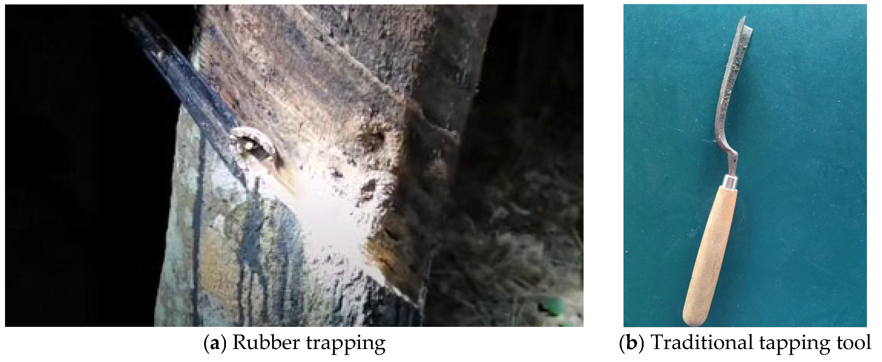
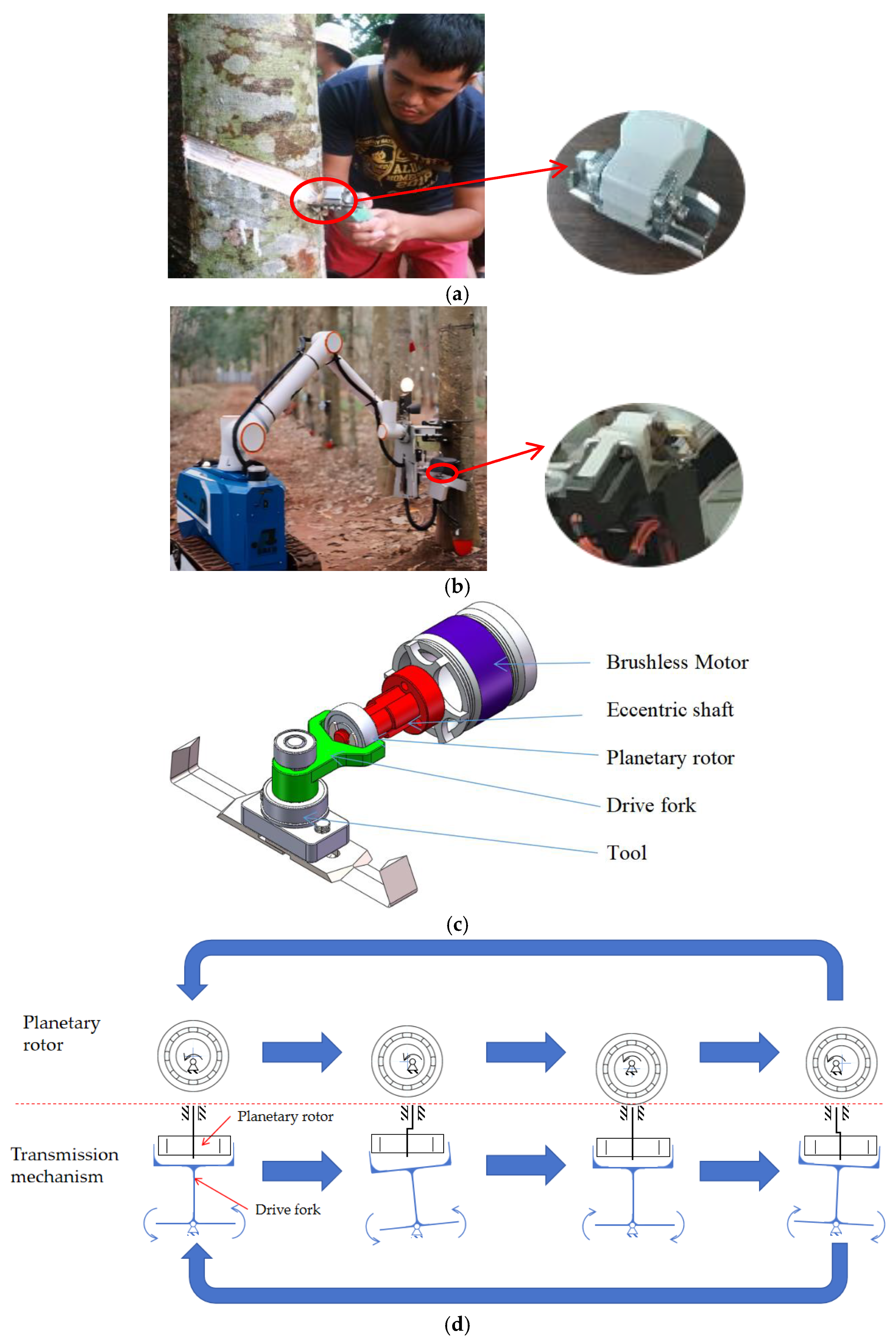
1. Introduction
2. Methods and Materials
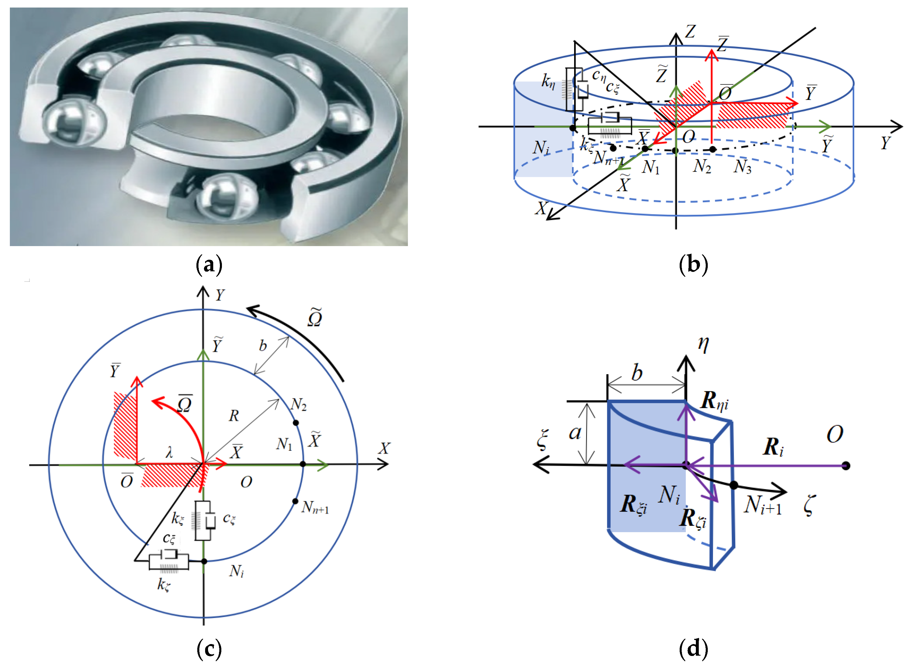
2.1. Overview of the Novel Eccentric 3D-REF Model
- (1)
- The element undergoes flexible deformation in ;
- (2)
- The element rigidly self rotates in ;
- (3)
- The element rigidly reaches eccentric revolution in .
2.2. The ANCF 3D-Beam Element
2.3. The Nonlinear Dynamic Differential Equation of Novel Eccentric 3D REF Model
2.3.1. Kinetic Energy of Planetary Rotor
2.3.2. Strain Energy of Planetary Rotor
2.3.3. Boundary Condition
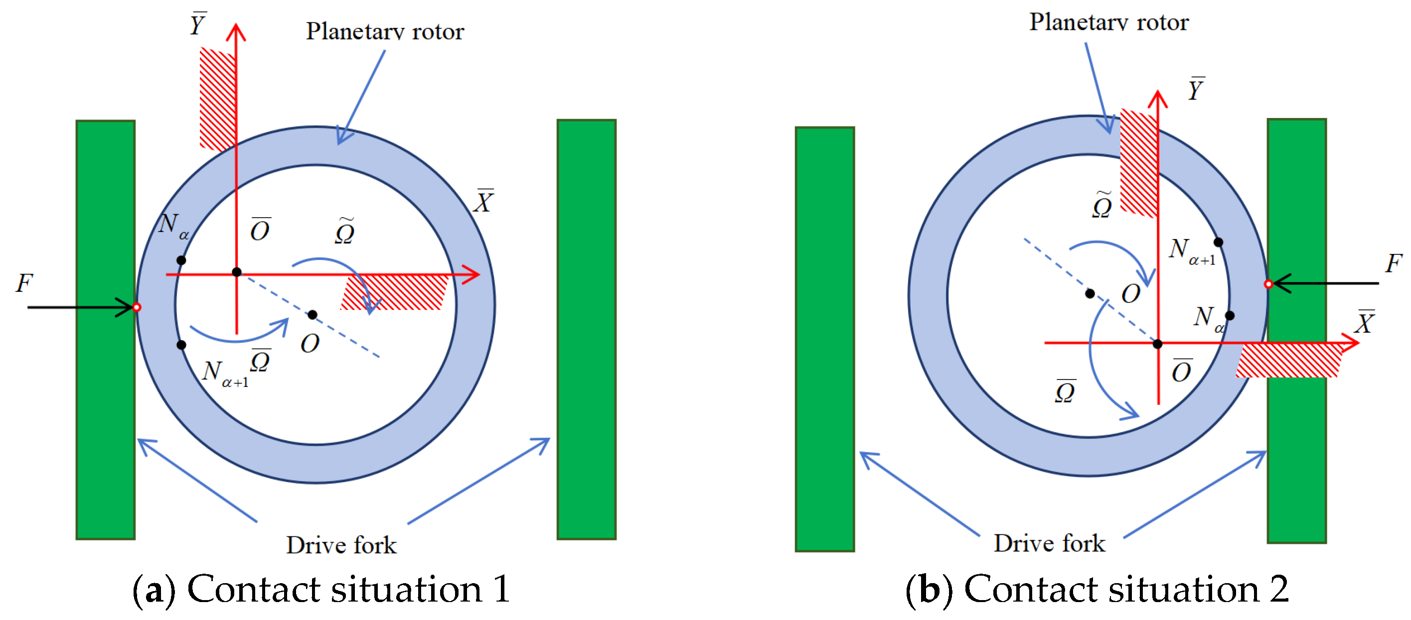
2.3.4. External Load
2.3.5. Nonlinear Dynamic Differential Equation
2.4. Numerical Calculation Method for Characteristic Multipliers
2.5. Initial Parameters of Planetary Rotor
3. Verification and Experiment
3.1. Theoretical Verification
3.1.1. Vibration of Uniformly Rotating Circular Ring Model
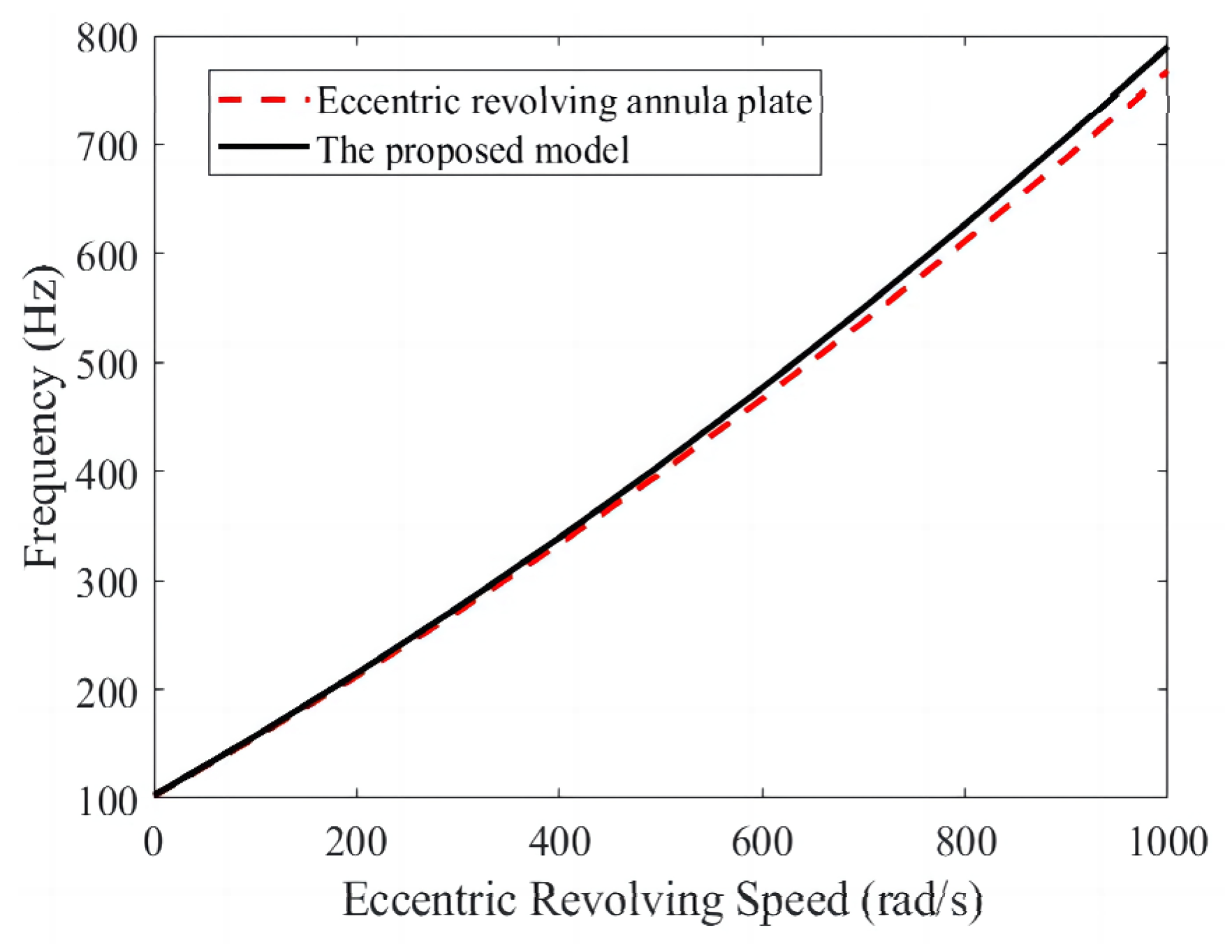
3.1.2. Rigid-Body Vibration Mode of Uniformly Eccentric Revolving Annular Plate
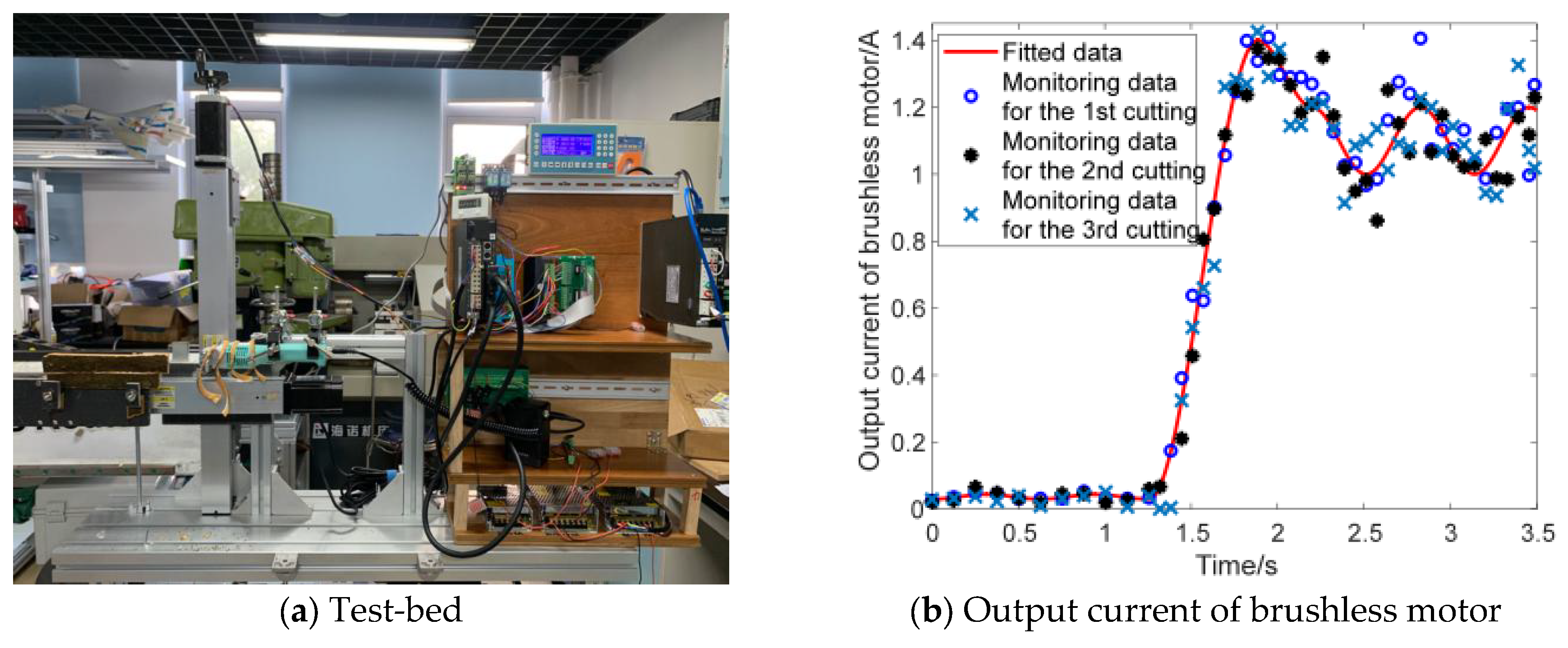
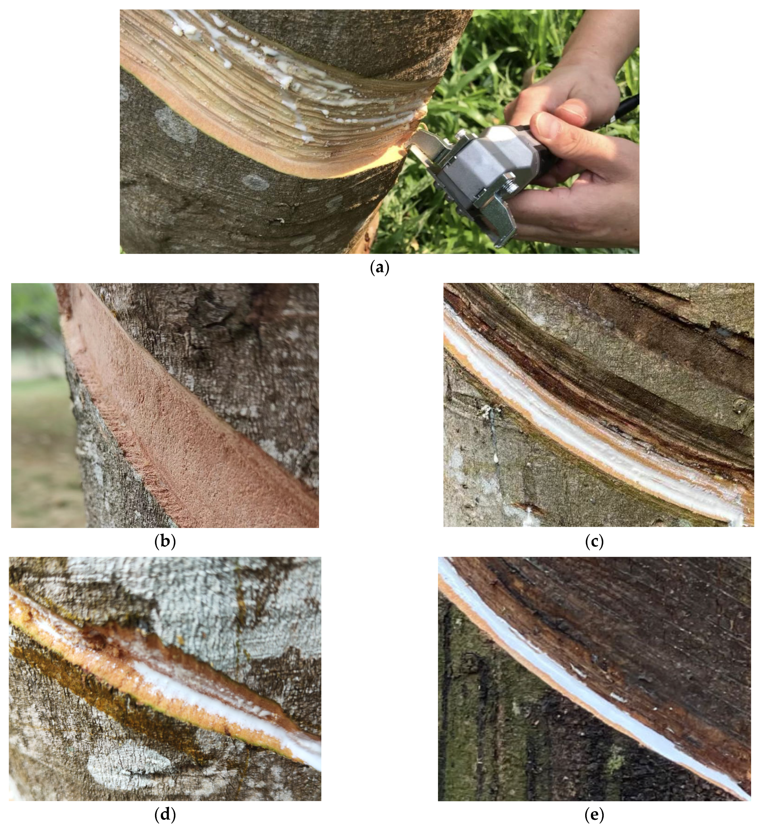
3.2. Stability Analysis and Experimental Analysis of the Planetary Rotor in the Rubber Tapping Machinery
4. Conclusions
Author Contributions
Funding
Data Availability Statement
Acknowledgments
Conflicts of Interest
Abbreviations
Appendix A
Appendix B
References
- Farag, N.H.; Pan, J. Modal characteristics of in-plane vibration of circular plates clamped at the outer edge. J. Acoust. Soc. Am. 2003, 113, 1935–1946. [Google Scholar] [CrossRef]
- Kim, C.B.; Cho, H.S.; Beom, H.G. Exact solutions of in-plane natural vibration of a circular plate with outer edge restrained elastically. J. Sound Vib. 2012, 331, 2173–2189. [Google Scholar] [CrossRef]
- Wang, Z.M.; Wang, Z.; Zhang, R. Transverse vibration analysis of spinning circular plate based on differential quadrature method. J. Vib. Shock 2014, 33, 125–129. (In Chinese) [Google Scholar] [CrossRef]
- Żur, K.K. Free vibration analysis of elastically supported functionally graded annular plates via quasi-Green’s function method. Compos. Part B Eng. 2018, 144, 37–55. [Google Scholar] [CrossRef]
- Tian, W.M.; Shi, M.J.; Tan, H.Y.; Wu, J.L.; Hao, B.Z. Structure and Development of Rubber Tree Bark, 1st ed.; Science Press: Beijing, China, 2015. (In Chinese) [Google Scholar]
- Zhang, X.R.; Wen, Z.T.; Zhang, Z.F.; Sun, Z.J.; Zhang, H.; Liu, J.X. Design and test of automatic rubber-tapping device with spiral movement. Trans. Chin. Soc. Agric. Mach. 2023, 54, 169–179. (In Chinese) [Google Scholar] [CrossRef]
- Soumahin, E.F.; Chantal, E.K.M.; N’dri, A.A.E.; Kouadio, Y.J.; Obouayeba, S. Influence of tapping time on rubber yield and the physiological status of rubber trees southeastern Côte d’Ivoire in a context of climate change. Int. J. Agric. Pol. Res. 2022, 10, 134–146. [Google Scholar] [CrossRef]
- Fang, J.; Shi, Y.; Cao, J.; Sun, Y.; Zhang, W. Active navigation system for a rubber-tapping robot based on trunk detection. Remote. Sens. 2023, 15, 3717. [Google Scholar] [CrossRef]
- Yang, H.; Sun, Z.; Liu, J.; Zhang, Z.; Zhang, X. The development of rubber tapping machines in intelligent agriculture: A review. Appl. Sci. 2022, 12, 9304. [Google Scholar] [CrossRef]
- Zhou, H.; Zhang, S.; Zhang, J.; Zhang, C.; Wang, S.; Zhai, Y.; Li, W. Design, development, and field evaluation of a rubber tapping robot. J. Field Robot. 2021, 39, 28–54. [Google Scholar] [CrossRef]
- Nie, F.; Zhang, W.; Wang, Y.; Shi, Y.; Huang, Q. A forest 3D Lidar SLAM system for rubber-tapping robot based on trunk center atlas. IEEE/ASME Trans. Mechatron. 2022, 27, 2623–2633. [Google Scholar] [CrossRef]
- Zhang, C.; Yong, L.; Chen, Y.; Zhang, S.; Ge, L.; Wang, S.; Li, W. A rubber-tapping robot forest navigation and information collection system based on 2D LiDAR and a gyroscope. Sensors 2019, 19, 2136. [Google Scholar] [CrossRef] [PubMed]
- Wang, S.; Zhou, H.; Zhang, C.; Ge, L.; Li, W.; Yuan, T.; Zhang, W.; Zhang, J. Design, development and evaluation of latex harvesting robot based on flexible toggle. Robot. Auton. Syst. 2022, 147, 103906. [Google Scholar] [CrossRef]
- Zhang, X.R.; Cao, C.; Zhang, L.N.; Xing, J.J.; Liu, J.X.; Dong, X.H. Design and Test of Profiling Progressive Natural Rubber Automatic Tapping Machine. Trans. Chin. Soc. Agric. Mach. 2022, 53, 99–108. (In Chinese) [Google Scholar] [CrossRef]
- Gao, K.K.; Sun, J.H.; Gao, F.; Jiao, J. Tapping error analysis and precision control of fixed tapping robot. Trans. Chin. Soc. Agric. Mach. 2021, 37, 44–50. (In Chinese) [Google Scholar] [CrossRef]
- Wen, X.Y.; Hong, Y.M.; Xiong, J.M.; Yu, Y.G.; Tan, J.H.; Meng, X.B. Design and experiment of fixed automatic natural rubber tapping machine. Trans. Chin. Soc. Agric. Mach. 2023, 54 (Suppl. S2), 128–135. (In Chinese) [Google Scholar] [CrossRef]
- Kamil, M.F.M.; Zakaria, W.N.W.; Tomari, M.R.M.; Sek, T.K.; Zainal, N. Design of automated rubber tapping mechanism. IOP Conf. Ser. Mater. Sci. Eng. 2020, 917, 012016. [Google Scholar] [CrossRef]
- Sun, Z.J.; Xing, J.J.; Hu, H.N.; Zhang, X.R.; Dong, X.H.; Deng, Y.G. Research on recognition and planning of tapping trajectory of natural rubber tree based on machine vision. J. Chin. Agric. Mech. 2022, 43, 102–108. (In Chinese) [Google Scholar] [CrossRef]
- Wongtanawijit, R.; Khaorapapong, T. Rubber tapping line detection in near-range images via customized YOLO and U-Net branches with parallel aggregation heads convolutional neural network. Neural Comput. Appl. 2022, 34, 20611–20627. [Google Scholar] [CrossRef]
- Wongtanawijit, R.; Khaorapapong, T. Nighttime rubber tapping line detection in near-range images. Multimed. Tools Appl. 2021, 80, 29401–29422. [Google Scholar] [CrossRef]
- Zhang, C.L.; Li, D.C.; Zhang, S.L.; Shui, Y.; Tan, Y.Z.; Li, W. Design and test of three-coordinate linkage natural rubber tapping device based on laser ranging. Trans. Chin. Soc. Agric. Mach. 2019, 50, 121–127. (In Chinese) [Google Scholar] [CrossRef]
- Yang, H.; Chen, Y.; Liu, J.; Zhang, Z.; Zhang, X. A 3D lidar SLAM system based on semantic segmentation for rubber-tapping robot. Forests 2023, 14, 1856. [Google Scholar] [CrossRef]
- Xu, W.X.; Zhang, L.C. Ultrasonic vibration-assisted machining: Principle, design and application. Adv. Manuf. 2015, 3, 173–192. [Google Scholar] [CrossRef]
- Bai, W.; Roy, A.; Guo, L.; Xu, J.; Silberschmidt, V.V. Silberschmidt. Analytical prediction of frictional behaviour and shear angle in vibration-assisted cutting. J. Manuf. Process. 2021, 62, 37–46. [Google Scholar] [CrossRef]
- Liang, X.L.; Zhang, C.B.; Cheung, C.F.; Wang, C.; Li, K.; Bulla, B. Micro/nano incremental material removal mechanisms in high-frequency ultrasonic vibration-assisted cutting of 316L stainless steel. Int. J. Mach. Tool Manu. 2023, 191, 104064. [Google Scholar] [CrossRef]
- Zhang, X.Y.; Peng, Z.L.; Liu, L.B. A transient cutting temperature prediction model for high-speed ultrasonic vibration turning. J. Manuf. Process. 2022, 83, 257–269. [Google Scholar] [CrossRef]
- Zou, L.; Yan, D.; Niu, Z.; Yuan, J.; Cheng, H.; Zheng, H. Parametric analysis and numerical optimisation of spinach root vibration shovel cutting using discrete element method. Comput. Electron. Agric. 2023, 212, 108138. [Google Scholar] [CrossRef]
- Shu, L.M.; Sugita, N. Analysis of fracture, force, and temperature in orthogonal elliptical vibration-assisted bone cutting. J. Comput. Electron. Agric. 2020, 103, 103599. [Google Scholar] [CrossRef]
- Chen, Y.; Pan, L.; Yin, Z.; Wu, Y. Effects of ultrasonic vibration-assisted machining methods on the surface polishing of silicon carbide. J. Mater. Sci. 2024, 59, 7700–7715. [Google Scholar] [CrossRef]
- Peng, Y.; Liang, Z.; Wu, Y.; Guo, Y.; Wang, C. Effect of vibration on surface and tool wear in ultrasonic vibration-assisted scratching of brittle materials. Int. J. Adv. Manuf. Technol. 2012, 59, 67–72. [Google Scholar] [CrossRef]
- Chinta, M.; Palazzolo, A.B. Stability and bifurcation of rotor motion in a magnetic bearing. J. Sound Vib. 1998, 214, 793–803. [Google Scholar] [CrossRef]
- Tiwari, M.; Gupta, K.; Prakash, O. Effect of radial internal clearance of a ball bearing on the dynamics of a balanced horizontal rotor. J. Sound Vib. 2000, 238, 723–756. [Google Scholar] [CrossRef]
- Rafsanjani, A.; Abbasion, S.; Farshidianfar, A.; Moeenfard, H. Nonlinear dynamic modeling of surface defects in rolling element bearing systems. J. Sound Vib. 2009, 319, 1150–1174. [Google Scholar] [CrossRef]
- Tu, W.B.; Liang, J.; Yu, W.N. Motion stability analysis of cage of rolling bearing under the variable-speed condition. Nonlinear Dyn. 2023, 111, 11045–11063. [Google Scholar] [CrossRef]
- Cooley, C.G.; Parker, R.G. Vibration of high-speed rotating rings coupled to space-fixed stiffnesses. J. Sound Vib. 2014, 333, 2631–2648. [Google Scholar] [CrossRef]
- Liu, Z.; Gao, Q. Development and parameter identification of the flexible beam on elastic continuous tire model for a heavy-loaded radial tire. J. Vib. Control 2018, 24, 5233–5248. [Google Scholar] [CrossRef]
- Liu, J.; Tang, C.K.; Shao, Y.M. An innovative dynamic model for vibration analysis of a flexible roller bearing. Mech. Mach. Theory 2019, 135, 27–39. [Google Scholar] [CrossRef]
- Viitala, R. Minimizing the bearing inner ring roundness error with installation shaft 3D grinding to reduce rotor subcritical response. CIRP J. Manuf. Sci. Technol. 2020, 30, 140–148. [Google Scholar] [CrossRef]
- Fan, B.; Wang, Z.M. Vibration analysis of radial tire using the 3D rotating hyperelastic composite REF based on ANCF. Appl. Math. Model. 2024, 126, 206–231. [Google Scholar] [CrossRef]
- Chen, X.Z.; Zhang, D.G.; Li, L. Dynamic analysis of rotating curved beams by using absolute nodal coordinate formulation based on radial point interpolation method. J. Sound Vib. 2019, 441, 63–83. [Google Scholar] [CrossRef]
- Kindt, P.; Sas, P.; Desmet, W. Development and validation of a three-dimensional ring-based structural tyre model. J. Sound Vib. 2009, 326, 852–869. [Google Scholar] [CrossRef]
- Wei, Y.T.; Liu, Z.; Zhou, F.Q.; Zhao, C.L. Three-dimensional REF model of tire including the out-of-plane vibration. J. Vib. Eng. 2016, 29, 795–803. (In Chinese) [Google Scholar] [CrossRef]
- Sopanen, J.; Mikkola, A. Dynamic model of a deep-groove ball bearing including localized and distributed defects. Part 1: Theory. Proc. Inst. Mech. Eng. Part K J. Multi-Body Dyn. 2003, 217, 201–211. [Google Scholar] [CrossRef]
- Sopanen, J.; Mikkola, A. Dynamic model of a deep-groove ball bearing including localized and distributed defects. Part 2: Implementation and results. Proc. Inst. Mech. Eng. Part K J. Multi-Body Dyn. 2003, 217, 213–223. [Google Scholar] [CrossRef]
- Vu, T.D.; Duhamel, D.; Abbadi, Z.; Yin, H.-P.; Gaudin, A. A nonlinear circular ring model with rotating effects for tire vibrations. J. Sound Vib. 2016, 388, 245–271. [Google Scholar] [CrossRef]
- Chung, J.T.; Heo, J.W.; Han, C.S. Natural frequencies of a spinning disk misaligned with the axis of rotation. J. Sound Vib. 2003, 260, 763–775. [Google Scholar] [CrossRef]


| Parameter | Symbol | Value | Unit |
|---|---|---|---|
| Radius | 6.8 | mm | |
| Radial thickness | 2.5 | mm | |
| Transverse thickness | 1.2 | mm | |
| Elastic modulus of outer ring | 207 | GPa | |
| Poisson’s ratio | 0.3 | - | |
| Density | 7810 | kg/m3 | |
| Eccentricity | 0.6 | mm |
| Parameter | Symbol | Value | Unit |
|---|---|---|---|
| Radius | 0.285 | m | |
| Radial thickness | 0.01 | mm | |
| Transverse thickness | 0.085 | mm | |
| Elastic modulus | 2.6611 | GPa | |
| Poisson’s ratio | 0.3 | - | |
| Density | 1160.7 | kg/m3 | |
| Spring stiffness | 4.35 | MPa | |
| 0.319 | MPa | ||
| 0 | MPa |
| Parameter | Symbol | Value | Unit |
|---|---|---|---|
| Radius | 40 | mm | |
| Radial thickness | 50 | mm | |
| Transverse thickness | 1.2 | mm | |
| Elastic modulus | 6.55 | MPa | |
| Poisson’s ratio | 0.3 | - | |
| Density | 1200 | kg/m3 | |
| Eccentricity | 13 | mm | |
| Revolving speed | 1000 | rad/s |
Disclaimer/Publisher’s Note: The statements, opinions and data contained in all publications are solely those of the individual author(s) and contributor(s) and not of MDPI and/or the editor(s). MDPI and/or the editor(s) disclaim responsibility for any injury to people or property resulting from any ideas, methods, instructions or products referred to in the content. |
© 2024 by the authors. Licensee MDPI, Basel, Switzerland. This article is an open access article distributed under the terms and conditions of the Creative Commons Attribution (CC BY) license (https://creativecommons.org/licenses/by/4.0/).
Share and Cite
Cao, J.; Fan, B.; Xiao, S.; Su, X. Stability Analysis of Planetary Rotor with Variable Speed Self Rotation and Uniform Eccentric Revolution in the Rubber Tapping Machinery. Forests 2024, 15, 1071. https://doi.org/10.3390/f15061071
Cao J, Fan B, Xiao S, Su X. Stability Analysis of Planetary Rotor with Variable Speed Self Rotation and Uniform Eccentric Revolution in the Rubber Tapping Machinery. Forests. 2024; 15(6):1071. https://doi.org/10.3390/f15061071
Chicago/Turabian StyleCao, Jianhua, Bo Fan, Suwei Xiao, and Xin Su. 2024. "Stability Analysis of Planetary Rotor with Variable Speed Self Rotation and Uniform Eccentric Revolution in the Rubber Tapping Machinery" Forests 15, no. 6: 1071. https://doi.org/10.3390/f15061071
APA StyleCao, J., Fan, B., Xiao, S., & Su, X. (2024). Stability Analysis of Planetary Rotor with Variable Speed Self Rotation and Uniform Eccentric Revolution in the Rubber Tapping Machinery. Forests, 15(6), 1071. https://doi.org/10.3390/f15061071