Improving the Site Index and Stand Basal Area Model of Picea asperata Mast. by Considering Climate Effects

Abstract

The stand basal area, closely related to age, site quality, and stand density, is an important factor for predicting forest growth and yield. The accurate estimation of site quality is especially a key component in the stand basal area model. We utilized sample plots with Picea asperata Mast. as the dominant species in the multi-period National Forest Inventory (NFI) dataset to establish a site index (SI) model including climate effects through the difference form of theoretical growth equations and mixed-effects models. We combined the SI calculated from the SI model, stand age, and stand density index to construct a basal area growth model for Picea asperata Mast. stands. The results show that the Korf model is the best SI base model for Picea asperata Mast. The mean temperatures in summer and winter precipitation were used as the fixed parameters to construct a nonlinear model. Ultimately, elevation, origin, and region, as random effects, were incorporated into the mixed-effects model. The coefficients (R²) of determination of the base model, the nonlinear model including climate, and the nonlinear mixed-effects model are 0.869, 0.899, and 0.921, with root-mean-square errors (RMSEs) of 1.320, 1.315, and 1.301, respectively. Among the basal area models, the Richards model has higher precision. And the basal area model including an SI incorporating climatic factors had a higher determination coefficient (R²) of 0.918 than that of the model including an SI without considering climatic effects. The mixed-effects model incorporating climatic and topographic factors shows a better fitting performance of SI, resulting in a higher precision of the basal area model. This indicates that in the development of forest growth models, both biophysical and climatic factors should be comprehensively considered.

1. Introduction

Stand growth and yield models, as fundamental tools for studying the patterns of forest growth changes and predicting the growth and yield of stands, are closely linked to age, site quality, and stand density [1,2]. In the system for predicting stand growth and yield, the stand basal area serves not only as a critical variable for estimating volume [3,4] but also as a primary factor in assessments [5]. Due to its high stability and predictability, research on the growth model of the stand basal area is a central focus in the modeling of stand measurement factors [4,5]. The stand basal area, intimately linked to species and stand productivity [6], is widely employed in estimating the dynamic changes in forest structure and resources and forms the foundation for formulating forest management plans [7].

When constructing a stand basal area model, the stand age, site quality, and stand density are pivotal variables [8]. The growth rates of a stand basal area vary significantly across different ages, with stand structure and intra-stand competition influencing basal area growth at varying stand ages [5]. Site quality impacts land productivity [9,10], with studies indicating that the magnitude of the basal area is influenced by site quality and initial density [11], and its growth rate is also affected by density [12,13]. Stand age and density are variables that can be easily measured; thus, accurately estimating site quality is a crucial component in developing a stand basal area model [14]. The site index (SI), established using the height–age relationship, serves as an indicator of site quality, elucidating the variations in productivity among stands [15]. Given that the SI integrates numerous factors and is commonly regarded as independent of density [16], it most directly reflects the potential growth differences in stands [17]. A precise estimation of the SI is essential to avoid introducing biases into growth models, which underpin forest management decisions [14].

The construction of a site index can be achieved through the use of static equations and dynamic equations that accommodate variable reference ages [18]. Static equations are highly contingent upon the reference age, with the function value representing the dominant height at the fixed reference age, whereas dynamic equations are capable of providing simultaneous estimates for tree height growth and site index [19], offering a distinct advantage over static equations in the fitting of site index models [20]. The algebraic difference approach (ADA) is a frequently utilized method for deriving dynamic site index equations. Bailey et al. [21] proposed the ADA, which involves establishing difference equations by assigning certain parameters within the growth equations as free parameters, thereby constructing polymorphic and dynamic site index models [22,23].

In this study, we utilized mixed-effects models to establish a site index model. Recently, mixed-effects model approaches are increasingly applied in developing various forest models [19,24]. The conventional ordinary least squares method, following the assumption of independent observations, provides appropriate parameter estimates for the population mean [25]. However, when significant differences exist between groups, the variance becomes biased [26]. Given the extensive and broad scope of the study area, the nonlinear mixed-effects (NLMEs) modeling approach was adopted to reduce biases by considering inter-group differences [25,27]. Comprising fixed and random effect parameters, NLMEs address autocorrelation issues in datasets [28], where their variance–covariance structure more effectively analyzes hierarchically structured data, thereby enhancing the model’s predictive accuracy [29].

The climate exerts a significant influence on forest growth [6,30]. It impacts crucial physiological and phenological processes in trees [31,32], leading to shifts in species distribution, forest composition, and productivity [33,34]. A better understanding of the relationship between tree growth and the climate may aid in forecasting the potential impacts of climate change on forest ecosystems [6,35]. Some researchers have demonstrated that the site index is influenced by environmental factors and forest management [36,37], while in the current scenario, changes in climatic conditions introduce uncertainty in estimating site quality [38]. As a countermeasure, scholars have incorporated climate variables into the site index model, developing a climate-sensitive site index [32]. This research investigates the impact of the climate on site quality by incorporating climate factors reflecting temperature and precipitation as random effects into the site index model.

Picea asperata Mast. is extensively distributed across the cold temperate and temperate high-mountain and subalpine regions of the Northern Hemisphere, being a primary species in northern coniferous forests and subalpine coniferous forests. Studies indicate that Picea asperata Mast. exhibits significant growth and phenological differences, reflecting the impact of the growth environment [31]. The climate is a crucial factor affecting the systematics and morphological differentiation of Picea asperata Mast. [39]; hence, incorporating climatic factors in constructing growth models for this species is vital.

Utilizing the site index as an indicator of site quality, and integrating difference equations and mixed-effects models, this research conducts an evaluation study on the site quality of Picea asperata Mast. inclusive of climatic effects; employing the site index along with the stand age and stand density index, a growth model for the basal area of Picea asperata Mast. stands are constructed, providing a theoretical basis for the management measures taken by forest operators under the influence of the climate. The specific objectives of this study are as follows: (1) to construct the DBH–tree height model and calculate the stand dominant height of Picea asperata Mast.; (2) to analyze the impact of the climate on tree height (site productivity) growth; (3) to establish a Picea asperata Mast. SI model incorporating climatic variables; and (4) to develop a stand basal area model of Picea asperata Mast. stands.

2. Materials and Methods

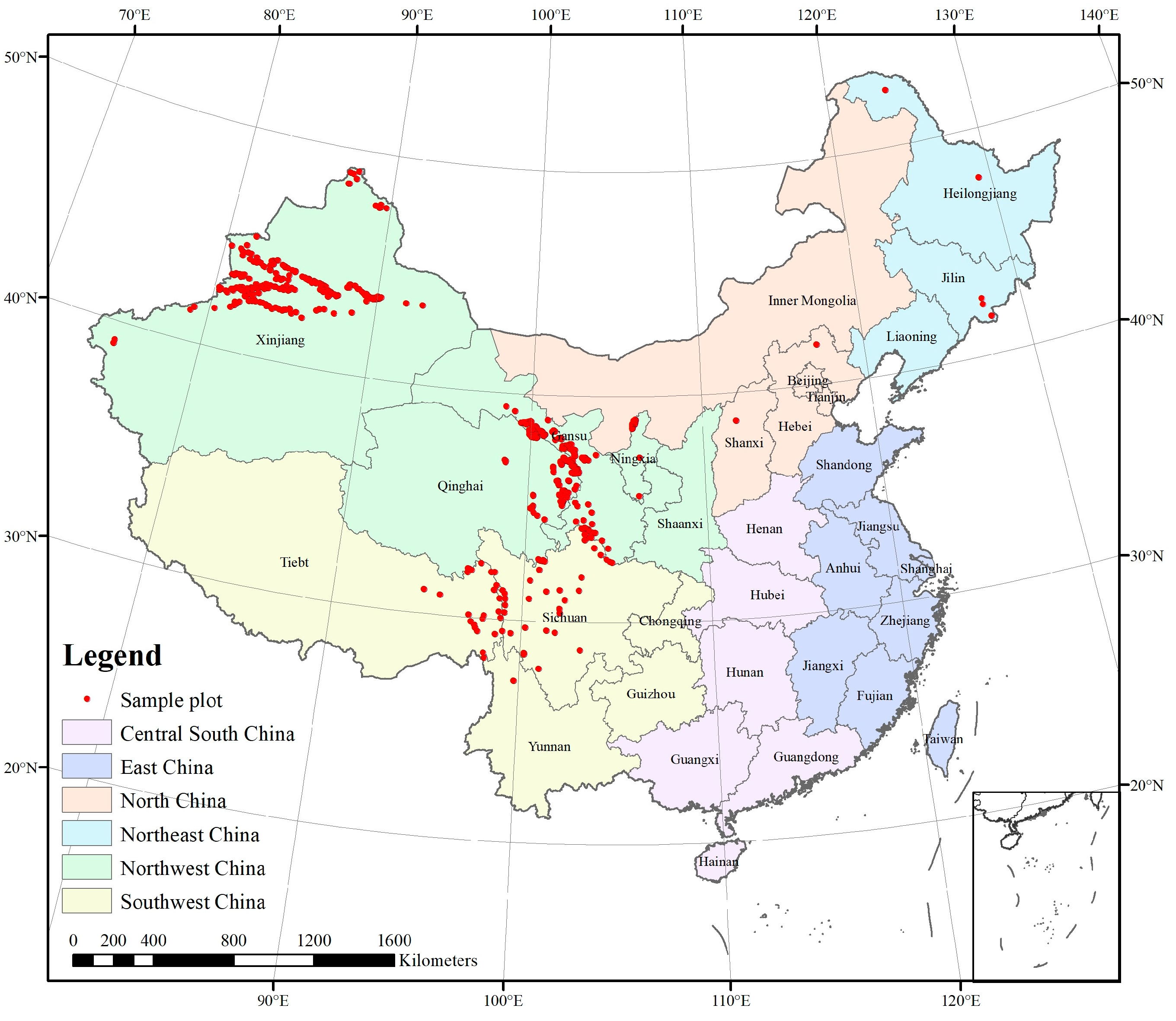
2.1. Data Collection

The data for this study were derived from the multi-period National Forest Inventory (NFI) dataset spanning 1999–2003, 2004–2008, 2009–2013, and 2014–2018 in China. We focused our analysis on forest plot data from the NFI data where the dominant tree species—defined as a tree species constituting more than 65% of the total stock in the sample plot—is Picea asperata Mast. A total of 660 plots were selected, as illustrated in Figure 1, with the main factor statistical information presented in

Table 1. Summary of main factors in 660 plots.

Variable Symbol	Variable	Mean	Median	Min.	Max.
H	Tree height/m	15.6	14.9	2.0	30.5
BA	Stand basal area/(m2·ha−1)	18.86	19.00	0.12	63.68
N	Number of trees per hectare	716.66	575	12	4383
T	Stand average age/year	109	107	8	280
Elev	Elevation (m)	2748	2780	310	4700
Slope-A	Slope aspect	/	/	/	/
Slope-D	Slope degree	29.32	30	0	80

.

The climatic data were referenced from an open access software package, ClimateAP (v3.10, the University of British Columbia, Vancouver, BC Canada), developed by Wang et al. [40]. We extracted the annual meteorological data for a total of 20 years, from 1999 to 2018, based on the coordinate information of each plot in the NFI. We calculated it according to the average values of four time periods from 1999 to 2003, 2004 to 2008, 2009 to 2013, and 2014 to 2018 as meteorological factors. The descriptions and summaries of these 16 climatic variables are compiled into

Table A1. Summary and description of climatic factors.

Variable Symbol	Variable	Mean	Median	Min.	Max.
Tmax_wt	Mean maximum temperature in the winter (°C)	−2.678	−2.320	−18.300	9.340
Tmax_sm	Mean maximum temperature in the summer (°C)	18.136	17.860	11.920	25.960
Tmin_wt	Mean minimum temperature in the winter (°C)	−15.637	−15.640	−33.940	−3.860
Tmin_sm	Mean minimum temperature in the summer (°C)	7.042	6.860	1.660	14.360
Tave_wt	Mean temperature in the winter (°C)	−9.157	−9.200	−26.120	2.760
Tave_sm	Mean temperature in the summer (°C)	12.588	12.360	7.060	19.760
PPT_wt	Winter precipitation (mm)	22.468	11.400	1.000	199.400
PPT_sm	Summer precipitation (mm)	288.540	282.600	4.800	784.000
MAT	Mean annual temperature (°C)	2.263	2.190	−3.800	9.820
MWMT	Mean warmest month temperature (°C)	13.643	13.400	8.140	21.700
MCMT	Mean coldest month temperature (°C)	−11.196	−11.220	−28.420	1.520
TD	Temperature difference between MWMT and MCMT, or continentality (°C)	24.838	24.600	14.960	46.100
MAP	Mean annual precipitation (mm)	550.924	528.400	6.000	1407.800
AHM	Annual heat:moisture index (MAT + 10)/(MAP/1000))	26.443	23.110	9.580	1055.780
Eref	Hargreaves reference evaporation (mm)	608.027	604.600	372.400	1039.400
CMD	Hargreaves climatic moisture deficit (mm)	184.868	174.600	7.400	601.000

in Appendix A.

2.2. DBH–Tree Height Model and Stand Dominant Height

In forestry surveys, tree height and diameter at breast height are the most important tree-measuring factors. However, due to the difficulty in measuring tree height, it is common to select several sample trees in each plot to measure their heights and construct a height–diameter model for calculating the missing values of the tree height within the plot [41,42]. Given the lack of dominant height data in Chinese forest inventory data [43], we utilized a height–diameter model to identify the top 20% thickest trees (i.e., dominant trees) in each stand, using their average height as the dominant height for each plot [44,45].

Studies have demonstrated that mixed-effects models built upon the Richards equation provide the optimal fit for tree height [45]. Consequently, we adopt this approach, employing 660 plot datasets partitioned into training and testing sets in a 4:1 ratio. Additionally, we integrated region and origin as random effects to construct a mixed-effects model for spruce height–diameter relationships, utilizing this model to predict individual tree heights.

The nonlinear mixed effects model (NLMEM) is a statistical model that incorporates both fixed effects and random effects to analyze data with hierarchical structures or repeated measures [46]. This model is adept at capturing nonlinear relationships within the data and accommodating variability among individuals. The mathematical formulation of the model is as follows:

$$\left\{\begin{array}{l}{Y}_i=f(\beta ,\mu ,X_i)+{\epsilon }_i\\ \mu ~N(0,D)\\ {\epsilon }_i~N(0,R)\end{array}\right.$$

(1)

where Y_i and X_i are the dependent and independent variables of the ith stand type; ${\epsilon }_i$ is the error vector; $\beta ,\mu$ are the fixed and random effects parameters, respectively; D is the random effect variance–covariance matrix; and R is the random error variance–covariance matrix. The optimal random effect variance–covariance structure is selected from a diagonal matrix, a compound symmetric matrix, and a generalized positive definite matrix, where R can be expressed as follows:

$$R={\sigma }^2{G}_i^{0.5}{\Gamma }_i{G}_i^{0.5}$$

(2)

where σ² represents the variance of the residuals within the model, and G_i accounts for within-group variance heteroscedasticity, with its diagonal elements provided by the variance function. Additionally, ${\Gamma }_i$ accounts for within-group autocorrelations of the residual errors and is considered to be an identity matrix in the absence of time autocorrelation.

When applying the mixed model in validation datasets, the random parameters should be predicted. The calculation formula is as follows [46,47]:

$$\widehat{\mu }=\widehat{D}{\widehat{Z}}_i^T{({\widehat{R}}_i+{\widehat{Z}}_i\widehat{D}{\widehat{Z}}_i^T)}^{-1}{\widehat{e}}_i$$

(3)

where $\widehat{\mu }$ is the estimate of the random parameters for region i; $\widehat{D}$ is the estimate of D; ${\widehat{Z}}_i$ is the designed matrices for random effects, $Z_i=\frac{\partial (\beta ,\mu ,X_i)}{\partial \mu }{|}_{\widehat{\beta },\widehat{\mu }}$, ${\widehat{Z}}_i^T$ is the transpose of Z_i; ${\widehat{R}}_i$ is the estimate of R_i; and ${\widehat{e}}_i$ is the difference between the observed value and the predicted value calculated from the fixed effect parameter.

2.3. Site Index Model

2.3.1. Base Difference Model Selection

The relationship between tree height and age is nonlinear; hence, nonlinear mathematical models are commonly employed to describe it [19]. The site index method, based on stand age and dominant height data, quantifies site quality by establishing the corresponding dominant height at the reference age as the site index through related theoretical growth equations [14]. The algebraic difference approach, developed from the difference form of theoretical growth equations, generates polymorphic site index curves [28]. This method assumes different tree height–growth curves under varying site conditions, aligning more closely with biological characteristics [48]. Moreover, the algebraic difference approach provides a direct expression for the site index equation, facilitating its application.

Drawing on previous scholars’ work, we selected four theoretical equations for tree height growth, including Richards, Hossfeld, Logistic, and Korf equations [19,49]. By treating the parameters as free variables, we derived the difference form of the theoretical equations for the dominant height growth of Picea asperata Mast. stands using the algebraic difference method (

Table 2. Theoretical growth equation, corresponding difference form, and site index model.

Model	Theoretical Equations	Difference Form	SI Equations
Richards	$H=a\times {(1-e^{-bt})}^c$	$H=H_0\times {\left(\frac{1-e^{-bt}}{1-e^{-b{t}_0}}\right)}^c+\epsilon$	$SI=H_t\times {\left(\frac{1-e^{-bT}}{1-e^{-bt}}\right)}^c+\epsilon$
Hossfeld	$H=\frac{a\times t^c}{b+t^c}$	$H=\frac{a}{1-\left(1-\frac{a}{H_0}\right){\left(\frac{t_0}{t}\right)}^b}+\epsilon$	$SI=\frac{a}{1-\left(1-\frac{a}{H_t}\right){\left(\frac{t}{T}\right)}^b}+\epsilon$
Logistic	$H=\frac{a}{1+e^{b-ct}}$	$H=\frac{a}{(a/H_0-1)\times e^{c{t}_0-ct}+1}+\epsilon$	$SI=\frac{a}{(a/H_t-1)\times e^{ct-cT}+1}+\epsilon$
Korf	$H=a\times e^{-\frac{b}{t^c}}$	$H={H_0}^{t_0^c/t^c}\times a^{1-t_0^c/t^c}+\epsilon$	$SI={H_t}^{t^c/T^c}\times a^{1-t^c/T^c}+\epsilon$

In the theoretical growth equation, H represents dominant height and t represents age. In the corresponding difference equation, H and t represent the mean height and age of the stand in the later period, and H₀ and t₀ represent the mean height and age of the stand in the previous period. In the SI equation, SI is the site index, T is the base age, and H_t and t are the dominant height and age of real stands. a, b, and c are the parameters.

). During the fitting of the difference equation, the input data comprise dominant height and age data from two consecutive periods for the plots, where H₀ and t₀ are the mean height and age of stands in the previous period, and H and t are the mean height and age of stands in the later period. When converting it to a site index, let H₀ = H_t when t₀ = t; H = SI, and t = T, where SI represents the dominant height of Picea asperata Mast. at the reference age, T denotes the reference age of the Picea asperata Mast., t is the age of the Picea asperata Mast. at any given time, and H_t is the dominant height at time t. Substituting these variables into the difference equation and performing variable substitution yields the site index equation for Picea asperata Mast.

2.3.2. Difference Model Equations with Environmental Factors

In ecological and forestry research, it is common to link certain parameters within models to environmental variables, such as climatic conditions, to enable the model to reflect the impact of these environmental factors on biological processes, like tree growth [14,32,50]. We employed a multiple stepwise regression analysis to filter out environmental factors that significantly influence tree growth. These key environmental factors were then linked to model parameters to establish their mathematical relationships. The fundamental principle of multiple stepwise regression starts with a comprehensive model containing all potential independent variables, iteratively adding or removing variables to construct a simpler, more optimal model. At each step, the model’s adequacy was evaluated using the Akaike Information Criterion (AIC), with variables being eliminated based on the objective of minimizing the AIC value. The stepwise regression process halts when no further improvements to the model are evident, resulting in a selectively optimized model. The independent variables within this final model, deemed to significantly impact the dependent variable, are described using a regression equation [34]. We conducted significance tests on these variables’ regression coefficients and reassessed the model’s collinearity. Ultimately, variables that were significant in the regression analysis and contributed to a notable reduction in AIC were selected to determine the final model.

2.3.3. Nonlinear Mixed-Effects Model

The nonlinear mixed-effects model is described in Section 2.2. In the process of constructing a mixed-effects model, a crucial step is the formulation of the model’s two main effects—random effects and fixed effects [24]. In this study, we took climate factor as a fixed effect [14] and terrain factor and distribution area together as a random effect to fit [51]. The model was evaluated using goodness-of-fit indicators such as the Akaike Information Criterion (AIC), the Bayesian Information Criterion (BIC), and the likelihood ratio test (LRT), where smaller AIC and BIC values indicated a better model fit, and the LRT provided additional evidence regarding the significance of model improvements. However, an excessive number of independent variables and parameters can lead to model non-convergence. To avoid this issue, a parameter construction with fewer parameters and a convergent form are selected. In this study, we first filtered out significant factors related to the subject of research and then utilized the optimal base model for the testing of the simulations of multi-parameter effects.

2.4. Stand Basal Area Model

The growth and development of forest stands are influenced by their stand age, site quality, and the degree of utilization of stand resources [8]. Therefore, the construction of a stand basal area growth model should include three variables: site quality index, stand density index, and stand age. The Richards and Schumacher models are recognized as suitable for calculating a stand basal area [24]. Both models incorporate parameters that reflect the asymptotic value and growth rate of the basal area, offering favorable mathematical and biological interpretations [7,8,52]. In this study, we selected these two nonlinear models as candidate base models for simulating the stand basal area. In the model construction, we incorporated the average stand age (T), stand density index, and site quality index. The site quality index was represented by the site index SI calculated in the previous section, while the density index was represented by the stand density index (SDI) to derive the basal area growth model.

SDI refers to Reineke’s stand density index [53]. The SDI is given by

$$SDI=N{(D_0/D)}^{\beta }$$

(4)

where β is a parameter, which we set to 1.605 [54]; D₀ is the standard base diameter (the recommended value is 20 cm); D is the arithmetic mean diameter at the breast height of the stand; and N is the number of standing living trees per hectare, respectively.

Among the two models, the one that performs better will be chosen. The specific forms of the models are as follows:

$$BA=aS{I}^b{(1-e^{(-c{(SDI/1000)}^{d}T)})}^f$$

(5)

$$BA=aS{I}^b\times e^{-c/T}\times {(SDI/1000)}^d$$

(6)

where BA, T, SI, and SDI are the stand basal area, stand age, site index, and stand density index; and a, b, c, d, and f are coefficients, respectively.

2.5. Model Selection and Evaluation

In the modeling process, we divided all the data into modeling data and validation data according to 8:2 and evaluated the goodness of fit of the model and the accuracy of the validation dataset. In statistical modeling, evaluating model performance is a crucial step. To thoroughly assess the model’s goodness of fit and predictive capacity, we employed the following five criteria: Akaike Information Criterion (AIC), Bayesian Information Criterion (BIC), coefficient of determination (R²), root-mean-square error (RMSE), and Mean Absolute Error (MAE).

In this study, AIC and BIC were used to measure the model’s goodness of fit. AIC tends to favor models that offer the best fit to the data while avoiding overfitting; it penalizes model complexity but not as severely as the BIC. Building upon this, the BIC takes into account the sample size, thus imposing a more stringent penalty on the number of model parameters when the sample size is large, thereby favoring simpler models. Utilizing both of these criteria in the model selection process allows for a more comprehensive decision-making approach. Typically, the model with the smallest AIC and BIC values is selected during the model selection process. R² measures the model’s ability to explain the variability in the data; a value closer to 1 indicates a stronger explanatory power of the model. RMSE directly reflects the accuracy of the model’s predictions, with smaller values indicating smaller predictive errors. Together, these indicators provide a comprehensive framework for assessing model performance.

$$AIC=-2\ln (l)+2p$$

(7)

$$BIC=-2\ln (l)+\ln (n)\times p$$

(8)

$$RMSE=\sqrt{\frac{{\displaystyle {\sum }_{i=1}^n(y_i}-{\widehat{y}}_i{)}^2}{n}}$$

(9)

$$R^2=1-\frac{{\displaystyle {\sum }_{i=1}^n(y_i-}{\widehat{y}}_i{)}^2}{{\displaystyle {\sum }_{i=1}^n(}{y}_i-{\overline{y}}_i{)}^2}$$

(10)

$$MAE={\displaystyle {\sum }_{i=1}^n\left|\frac{y_i-{\widehat{y}}_i}{n}\right|}$$

(11)

where y_i is the measured value of the ith sample; ${\widehat{y}}_i$ is the predicted value of the ith sample; ${\overline{y}}_i$ is the average measured value; p is the number of parameters in the model; n is the number of samples; and l is the value of the model’s great likelihood function.

3. Results

3.1. Environmental Factor Selection

In this study, we employed a multiple stepwise regression model for factor selection. Tree height was utilized as the dependent variable, with 16 climatic factors, along with three topographic factors—elevation, slope degree, and slope aspect—and origin as independent variables to establish the stepwise regression model. Before executing the multiple stepwise regression, we normalized the data to ensure the reliability of the results. The results are shown in

Table 3. Multivariate stepwise regression analysis with tree height as the dependent variable and a summary of selected environmental factors.

Factor	Description	Mean	Median	Min.	Max.	Estimate	Std. Error	p Value
Tmax_sm	Mean maximum temperature in the summer (°C)	18.136	17.860	11.920	25.960	3.005	0.385	<0.001
Tave_sm	Mean temperature in the summer (°C)	12.588	12.360	7.060	19.760	−3.013	0.849	<0.001
PPT_sm	Summer precipitation (mm)	288.540	282.600	4.800	784.000	0.007	0.001	<0.001
PPT_wt	Winter precipitation (mm)	22.468	11.400	1.000	199.400	−0.072	0.001	<0.001
MWMT	Mean warmest month temperature (°C)	13.643	13.400	8.140	21.700	−1.266	0.587	<0.01
RH	Relative humidity (%)	57.587	57.800	43.800	72.200	0.579	0.057	<0.001
Elev	Elevation	2748	2780	310	4700	−0.457	0.201	<0.01
Origin	/	/	/	/	/	3.067	0.637	<0.001

, with elevation being the only topographic factor selected. Since random effects require categorical variables, elevation is graded, with nine levels per 500 m of one level.

The results reveal that six climatic variables—Tmax_sm, Tave_sm, PPT_sm, PPT_wt, MWMT, and RH—along with elevation and origin were selected. The standardized regression coefficients indicated that origin had the most substantial impact on tree height growth, followed by Tmax_sm and Tave_sm. Among the chosen factors, PPT_sm had the least influence on tree height.

3.2. DBH–Tree Height Model and Stand Dominant Height Fitting

We used the Richards model as the ba model to construct a mixed effect model to calculate the stand dominant height. The fitting results are shown in

Table 4. Parameter fitting and accuracy verification results of DBH–tree height model.

Parameter	Estimate	Std. Error	p Value	R2	RMSE	MAE
${\beta }_1$	29.902	1.852	<0.001	0.738	3.026	2.352
${\beta }_2$	0.032	0.004	<0.001
${\beta }_3$	1.162	0.066	<0.001

and Equation (12).

The results indicate that the developed model had an R² value of 0.738, an RMSE of 3.026, and an MAE of 2.352. The fitting results for each factor were significant.

$$\begin{array}{c}H=1.3+( {\beta }_1+{\mu }_1+{\mu }_2){(1-e^{-{\beta }_2\times D})}^{{\beta }_3}+\epsilon \\ \mu =\left[\begin{array}{l}{\mu }_1\\ {\mu }_2\end{array}\right]~N\left\{\left[\begin{array}{l}0\\ 0\end{array}\right],D=\left(\begin{array}{cc}8.281\times {10}^{-3}& 0\\ 0& 2.540\times {10}^{-1}\end{array}\right)\right\}\end{array}$$

(12)

Using Equation (12), we calculated the tree height of individual trees based on their diameter at breast height and selected the average height of the top 20% dominant trees to serve as the dominant height for the calculation of the site index.

3.3. Site Index Model Fitting

3.3.1. Base Difference Model Selection and Fitting

By fitting tree height–growth curves using theoretical growth equations and their corresponding difference equations, the results, as shown in

Table 5. Parameter fitting results and precision test of the four basic differential equations.

Model	Parameters	Estimate	Std. Error	AIC	BIC	R2	RMSE	MAE
Richards	b	0.060 *	0.005	5059.873	5075.554	0.846	1.338	0.580
	c	−0.155 *	0.065
Hossfeld	a	9.573 ***	1.089	5038.709	5054.389	0.860	1.327	0.597
	b	0.265 ***	0.083
Logistic	a	11.761 ***	1.849	5057.061	5072.741	0.846	1.338	0.586
	c	0.001 ***	0.006
Korf	a	7.505 **	1.244	5028.946	5044.626	0.869	1.320	0.595
	c	0.248 **	0.065

*** p < 0.001, ** p < 0.01, * p < 0.05.

, were filtered based on the principles of minimum AIC, BIC, and RMSE values. The findings indicate that the Korf model, with an AIC of 5028.946, a BIC of 5044.626, an RMSE of 1.320, and an MAE of 0.595, exhibited the best performance. Among the other three models, the logistic model showed inferior outcomes, while the remaining two models demonstrated slightly less optimal results compared to the Korf model but still achieved relatively good performance.

In this study, 80a was selected as the reference age. According to variable substitution, the site index model based on the Korf difference equation was calculated as follows:

$$S{I}_{base}={H_t}^{t^{0.248}/2.965}\times {7.505}^{1-t^{0.248}/2.965}+\epsilon$$

(13)

where SI_base is the dominant height of Picea asperata Mast. at the reference age of 80a, H_t is the actual stand height at age t, and $\epsilon$ is the error.

3.3.2. Difference Model Fitting with Climate Factors

The environmental factors selected were incorporated in a parameterized form into the difference equations, integrating the six climatic factors (Tmax_sm, Tave_sm, PPT_sm, PPT_wt, MWMT, and RH) in various combinations into the optimal base model, the Korf model. By comparing the R², RMSE, and MAE values of models with different combination forms, the results indicate that the model’s accuracy improved with the inclusion of Tave_sm and PPT_wt. The final model was determined, with its specific form presented below.

$$H={H_0}^{t_0^{c+m1\times Tave\_sm}/t^{c+m2\times PPT\_wt}}\times a^{1-t_0^c/t^c}+\epsilon$$

(14)

The obtained model had an RMSE of 1.315, an R² of 0.0.899, and an MAE of 0.594; the fitting results of each factor were significant.

Table 6. Parameter fitting and accuracy verification results of difference equations with climate effects.

Parameter	Estimate	Std. Error	p Value	R2	RMSE	MAE
a	7.495	0.874	<0.01	0.899	1.315	0.594
c	0.249	0.054	<0.01
m1	0.001	0.000	<0.05
m2	0.006	0.000	<0.05

shows the fitted values of each parameter of the model.

3.3.3. Nonlinear Mixed-Effects Model Fitting

On the foundation of parameterizing the climate factor model, random effects were introduced. The results of the stepwise regression analysis reveal that elevation was a significant topographic factor, and origin also exhibited a high degree of correlation with tree height. Consequently, elevation, origin, and region were selected as random effects. We employed AIC and BIC criteria to compare models and identify which factors significantly enhance the model’s goodness of fit. When introducing random effects into parameter c, we observed a very low standard deviation of random effects, indicating that the variability in the model was primarily explained by fixed effects, with limited explanatory power from random effects on data variability. Additionally, based on the AIC and BIC results, the introduction of random effects to c had a minimal impact on the model outcomes; hence, no random effects were added to parameter c; all random effects were applied to parameter a.

With one random parameter considered, the model converged entirely, showing the highest fitting accuracy for origin, with AIC and BIC being 4656.731, 4688.092, respectively. When two random parameters were introduced, with the model incorporating origin and region achieving the highest fitting accuracy, AIC and BIC were 4658.933 and 4695.522, respectively. Among combinations with three random parameters, and the model including origin, region and elevation had the highest fitting accuracy, with AIC and BIC values of 4654.190 and 4696.006, respectively. The results of the likelihood ratio test (LRT) indicate that models incorporating varying numbers of random factors differed significantly. Specifically, the model with two random factors showed a significant difference from the model with one random factor at the 0.05 level. Similarly, the model with three random factors also exhibited a significant difference when compared to the model with two random factors. Therefore, it was meaningful to include three random factors in the model (

Table 7. Model fitting results with different random effects.

Random Effect	AIC	BIC	LRT (Chisq)	p Value
Origin	4656.731	4688.092	/	/
Region	4671.483	4702.845	14.753	<0.001
Elev	4676.42	4707.78	4.9353	<0.001
Origin, region	4658.933	4695.522	19.485	<0.001
Elev, origin	4658.94	4695.525	0.0028	<0.001
Elev, region	4671.183	4707.772	12.247	<0.001
Origin, region, elev	4654.190	4696.006	18.993	<0.001

In the formula, LRT and p value are the results of the likelihood ratio test, and the LRT value is the corresponding Chi-square statistic. If the corresponding p value is less than 0.05, it indicates that the model is optimized by adding new factors.

).

In the model development, we sequentially introduced three types of random parameter covariance structures: the diagonal matrix, the compound symmetry matrix, and the generalized positive definite matrix. Through calculations, we determined that the diagonal matrix was the optimal structure for the variance–covariance of random effects, where the model incorporates multiple random effects, each with a standard deviation. This standard deviation represented the degree of variation in the random effects across different groups and is represented in Equation (15) as the variance matrix D (

Table 8. Fixed parameter fitting and accuracy evaluation of nonlinear mixed effect model.

Parameter	Estimate	Std. Error	R2	RMSE	MAE
a	7.9345	2.24656	0.921	1.301	0.588
c	0.3534	0.0600
m1	0.0001	0.0003
m2	0.0007	0.0003

).

$$\begin{array}{c}H={H_0}^{t_0^{0.3534+0.00010\times Tave\_sm}/t^{0.3534+0.00067\times PPT\_wt}}\times {(7.9345+{\mu }_1+{\mu }_2+{\mu }_3)}^{{1-t_0}^{0.3534}/t^{0.3534}}+\epsilon \\ \mu =\left[\begin{array}{l}{\mu }_1\\ {\mu }_2\\ {\mu }_3\end{array}\right]~N\left\{\left[\begin{array}{l}0\\ 0\\ 0\end{array}\right],D=\left(\begin{array}{ccc}9.37& 0& 0\\ 0& 6.400\times {10}^{-5}& 0\\ 0& 0& 1.672\times {10}^{-5}\end{array}\right)\right\}\end{array}$$

(15)

where ${\mu }_1$, ${\mu }_2$, and ${\mu }_3$ denote the random effects of origin, region, and elevation, respectively.

Therefore, the SI model of Picea asperata Mast., based on the nonlinear mixed-effects model, is as follows:

$$S{I}_{NLME}={H_t}^{t^{0.3534+0.00010\times Tave\_sm}{/80}^{0.3534+0.00067\times PPT\_wt}}\times {(7.9345+{\mu }_1+{\mu }_2+{\mu }_3)}^{1-t^{0.3534}/4.7049}+\epsilon$$

(16)

where SI_NLME is the dominant height of Picea asperata Mast. at the reference age of 80a, H_t is the actual stand height at age t, and $\epsilon$ is the error.

3.3.4. Comparison of Model Fitting Results

Transitioning from the basic difference model to the difference model with climate effects and the nonlinear mixed-effects model, the incorporation of climatic factors and random effects uniformly enhanced the precision of the models, as indicated by the accuracy verification metrics. The fitting conditions for each model are displayed in

Table 9. Comparison of different models.

No.	Model	R2	RMSE	MAE
Equation (13)	Basic difference model	0.869	1.320	0.595
Equation (14)	Difference model with climate effects	0.899	1.315	0.594
Equation (15)	Nonlinear mixed-effects model	0.921	1.301	0.588

. The RMSE values decreased from 3.315 to 2.774, the MAE values reduced from 1.866 to 1.519, and the R² value increased from 0.644 to 0.778.

3.4. Stand Basal Area Model Fitting

For the development of stand basal area growth models, we employed stand mean age (T), SDI, and SI as independent variables, with basal area serving as the dependent variable to construct four models based on Equations (5) and (6). These models underwent accuracy verification using both modeling and testing datasets. SI_NLME-BA1 and SI_NLME-BA2 were established using SI_NLME (Equation (16)) as the site quality factor, corresponding to the Richards and Schumacher basal area models inclusive of climate effects, whereas SI_base-BA1 and SI_base-BA2 were constructed using SI_base (Equation (13)), representing the models exclusive of climate effects. The fitting outcomes and precision of these models are delineated in

Table 10. The fitting results and accuracy verification of stand basal area parameters.

Data	Indicator	SINLME-BA1	SINLME-BA2	SIbase-BA1	SIbase-BA2
Parameters	a	41.530 *** (1.418)	23.078 *** (0.629)	30.360 *** (2.020)	16.426 *** (0.380)
	b	0.178 *** (0.009)	0.197 *** (0.010)	0.237 *** (0.018)	0.304 *** (0.011)
	c	0.001 *** (0.001)	11.998 *** (1.01)	0.001 * (0.001)	0.336 *** (0.207)
	d	5.832 *** (0.166)	0.954 *** (0.013)	7.645 *** (0.449)	0.954 *** (0.012)
	f	0.166 *** (0.005)	/	0.128 *** (0.007)	/
Model evaluation	AIC	7290.528	7372.389	7439.741	7464.774
	BIC	7321.89	7398.524	7470.863	7490.709
Modeling data	R2	0.918	0.905	0.891	0.889
	RMSE	3.407	3.822	4.011	4.064
	MAE	2.126	2.185	2.187	2.223
Validation data	R2	0.915	0.899	0.886	0.883
	RMSE	3.460	3.900	4.335	4.401
	MAE	2.197	2.208	2.265	2.359

*** p < 0.001, * p < 0.05. The values in parentheses represent standard errors.

.

As indicated in Table 10, within the basal area models that employ SI_NLME (Equation (16)), incorporating climate effects as a measure of site quality, SI_NLME-BA1 exhibits lower AIC and BIC values compared to SI_NLME-BA2, signifying superior performance and a better model fit of SI_NLME-BA1. The R² and RMSE values of SI_NLME-BA1 outperform those of SI_NLME-BA2 in both the modeling and testing datasets, indicating that SI_NLME-BA1 provides a better fit to the data and yields more accurate predictive results than SI_NLME-BA2, suggesting that the Richards model is more suitable for our research. In the case of basal area models that use SI_base (Equation (13)) as a site quality indicator, the same trend is observed where SI_base-BA1 surpasses SI_base-BA2 across all metrics. However, the accuracy of SI_base-BA1 and SI_base-BA2 is significantly lower than that of SI_NLME-BA2. The results demonstrate that incorporating climate effects into the site index enhances the overall fitting precision of the basal area models.

In this study, we evaluated the predictive performance of the models using scatter plots to compare predicted values against actual values, as illustrated in Figure 2. These charts vividly depict the relationship between model predictions and observed values, where the distribution of points near the ideal 1:1 line allows us to visually assess the model’s predictive bias and consistency. The figures reveal that the basal area models with climate effects exhibit a certain degree of accuracy and reliability.

4. Discussion

In our study, environmental factors such as the mean temperature in summer and winter precipitation were incorporated as fixed parameters, while elevation, origin, and region were introduced as random effects into the model. Research indicates that temperature and precipitation significantly impact forest productivity [55]. Temperature is often a primary limiting factor for mountain forest growth [56], where higher temperatures usually denote faster tree growth rates and lower mortality rates [6]. A study on black spruce revealed that its growth positively responds to warmer growing seasons [33], and it has been shown that the average temperature from March to September significantly affects the tree height of most species, suggesting that the temperature during the growing season is critical in defining the thermal ecological niche for specific species [32]. Warm temperatures and extended growing seasons promote photosynthesis and the allocation of carbohydrates to stems [35]. Studies also suggest that the climatic response of trees varies regionally, possibly reflecting different climatic limitations on tree growth across study areas [55]. Areas with less summer precipitation rely on winter precipitation for replenishment [57], while the negative response to winter precipitation in regions with abundant rainfall may reflect the indirect impact of excessive snow harming tree growth [58]. Additionally, snowfall is associated with a delayed onset of the growing season and reduced radial growth [59]. Elevation significantly influences ecological processes at a location, affecting the amount of solar radiation received [60], which in turn impacts the regional climate. Therefore, the spatial variation in elevation gradients is a key determinant of mountain vegetation patterns, species distributions, and ecological layouts [61]. Our study introduced origin as a random effect variable in the site index model, exploring its significant impact on stand growth dynamics. Natural and planted forests differ in growth patterns [16], and distinguishing these origins in the model allows for a more accurate prediction and understanding of basal area growth dynamics across forest types. Considering origin categorization in the model enhances predictive capability regarding future stand growth trends [62], which is essential for long-term forest resource planning and sustainable management.

This research utilized NFI data to develop a mixed-effects model that incorporates climate effects to describe the site index and established a stand basal area model. Many scholars have created predictive models for species’ site index and basal area equations, with site index model accuracies being around R² = 0.62–0.86 [63,64] and stand basal area model R² values being approximately 0.706–0.970 [5,7]. The site index developed in this study through the mixed-effects model achieved R² = 0.921, and the basal area model reached R² = 0.918, demonstrating good predictive accuracy.

Mixed-effects models offer greater flexibility than traditional nonlinear models [29]. In our study, we observed that incorporating climate factors into the model significantly enhanced the predictive performance compared to the basic difference model. Furthermore, introducing random effects into the model surpassed the performance of a nonlinear model that only considered parametric climate factors. This finding confirms the superiority of mixed-effects models in handling hierarchical forestry data, capturing fixed effects across sites and accounting for random variations [51]. The flexibility of this model type is particularly suitable for analyzing plot data with repeated observations over large regions, providing a more accurate and comprehensive method for forest resource management and ecological research [65].

The Richards and Schumacher models, commonly used for basal area calculations [24], contain parameters reflecting asymptotic values and growth rates, offering sound mathematical and biological interpretations [7,8,52]. While the Schumacher model is simple and convenient to compute, the Richards model effectively describes the nonlinear characteristics of stand growth [66]. Zhao et al.’s findings, which show higher accuracy for the Richards model over the Schumacher model in developing stand basal area models [7], resonate with our results, affirming the superior accuracy of the Richards model. This might be due to the Richards model containing more parameters, allowing it to flexibly adapt to complex relationships and nonlinear features in the data, capturing subtle variations to enhance model fits. Another possibility is that the Richards model is more suited to the data distribution in our study, better capturing these characteristics. Additionally, our research compared the application effects of the site index with and without climate effects in basal area equation modeling. The results show that incorporating climate factors into the site index model not only significantly improved the predictive accuracy of the site index itself but also significantly enhanced the accuracy of the basal area model based on this site index. This further confirms the important role of climate factors in predicting stand basal areas. By integrating climate variables into the site index model, we can more accurately reflect the complex relationship between stand growth and environmental conditions, providing a more precise tool for forest resource management and ecological assessment. This underscores the necessity of considering biophysical and climatic factors in the development of forest growth models for a comprehensive understanding of forest ecosystem dynamics.

5. Conclusions

This study utilized fixed plots dominated by Picea asperata Mast. from multi-temporal National Forest Inventory (NFI) data to establish a site index model that incorporates climate effects through difference equations and nonlinear mixed-effects models. Furthermore, it developed a model for the basal area of Picea asperata Mast. stands, incorporating the stand age, site index, and stand density index. The results indicate that the Korf model serves as the optimal base model for the Picea asperata Mast. site index, while the Richards model is more suitable for constructing the basal area model. The site index model established through the nonlinear mixed-effects model achieved an R² of 0.921, and the basal area model reached an R² of 0.918, indicating a high predictive accuracy. Temperature, precipitation, origin, and elevation significantly influenced the construction of the site index, and the inclusion of these factors enhanced the predictive accuracy of the basal area model. By integrating climate factors into the site index model, this research quantified the impact of climatic elements on site quality. Incorporating climate factors enables the model to reflect the influence of the climate, which is crucial for predicting the future impacts of climate change on forest ecosystems. This assists forest managers in analyzing the potential effects of climate change on forest productivity and in formulating appropriate management strategies.

References

1. Pretzsch, H.; Schütze, G. Tree Species Mixing Can Increase Stand Productivity, Density, and Growth Efficiency and Attenuate the Tradeoff between Density and Growth throughout the Whole Rotation. Ann. Bot. 2021, 128, 767–786. [Google Scholar] [CrossRef] [PubMed]
2. Fien, E.K.P.; Fraver, S.; Teets, A.; Weiskittel, A.R.; Hollinger, D.Y. Drivers of Individual Tree Growth and Mortality in an Uneven-Aged, Mixed-Species Conifer Forest. For. Ecol. Manag. 2019, 449, 117446. [Google Scholar] [CrossRef]
3. Rodríguez, F.; Pemán, J.; Aunós, Á. A Reduced Growth Model Based on Stand Basal Area. A Case for Hybrid Poplar Plantations in Northeast Spain. For. Ecol. Manag. 2010, 259, 2093–2102. [Google Scholar] [CrossRef]
4. Zhang, L.; Peng, C.; Dang, Q. Individual-Tree Basal Area Growth Models for Jack Pine and Black Spruce in Northern Ontario. For. Chron. 2004, 80, 366–374. [Google Scholar] [CrossRef]
5. He, H.; Zhu, G.; Ma, W.; Liu, F.; Zhang, X. Additivity of Stand Basal Area Predictions in Canopy Stratifications for Natural Oak Forests. For. Ecol. Manag. 2021, 492, 119246. [Google Scholar] [CrossRef]
6. Condés, S.; del Río, M.; Forrester, D.I.; Avdagić, A.; Bielak, K.; Bončina, A.; Bosela, M.; Hilmers, T.; Ibrahimspahić, A.; Drozdowski, S.; et al. Temperature Effect on Size Distributions in Spruce-Fir-Beech Mixed Stands across Europe. For. Ecol. Manag. 2022, 504, 119819. [Google Scholar] [CrossRef]
7. Zhao, L.; Li, C. Stand Basal Area Model for Cunninghamia Lanceolata (Lamb.) Hook. Plantations Based on a Multilevel Nonlinear Mixed-Effect Model across South-Eastern China. South. For. A J. For. Sci. 2013, 75, 41–50. [Google Scholar] [CrossRef]
8. Sun, H.; Zhang, J.; Duan, A.; He, C. A Review of Stand Basal Area Growth Models. For. Stud. China 2007, 9, 85–94. [Google Scholar] [CrossRef]
9. Ouyang, S.; Xiang, W.; Wang, X.; Xiao, W.; Chen, L.; Li, S.; Sun, H.; Deng, X.; Forrester, D.I.; Zeng, L.; et al. Effects of Stand Age, Richness and Density on Productivity in Subtropical Forests in China. J. Ecol. 2019, 107, 2266–2277. [Google Scholar] [CrossRef]
10. Zhao, X.; Feng, Z.; Zhou, Y.; Lin, Y. Key Technologies of Forest Resource Examination System Development in China. Engineering 2020, 6, 491–494. [Google Scholar] [CrossRef]
11. Weiskittel, A.R.; Kuehne, C. Evaluating and Modeling Variation in Site-Level Maximum Carrying Capacity of Mixed-Species Forest Stands in the Acadian Region of Northeastern North America. For. Chron. 2019, 95, 171–182. [Google Scholar] [CrossRef]
12. Antón-Fernández, C.; Burkhart, H.E.; Amateis, R.L. Modeling the Effects of Initial Spacing on Stand Basal Area Development of Loblolly Pine. For. Sci. 2012, 58, 95–105. [Google Scholar] [CrossRef]
13. Zhao, D.; Bullock, B.P.; Montes, C.R.; Wang, M. Rethinking Maximum Stand Basal Area and Maximum SDI from the Aspect of Stand Dynamics. For. Ecol. Manag. 2020, 475, 118462. [Google Scholar] [CrossRef]
14. Sharma, M. Climate Effects on Jack Pine and Black Spruce Productivity in Natural Origin Mixed Stands and Site Index Conversion Equations. Trees For. People 2021, 5, 100089. [Google Scholar] [CrossRef]
15. Berrill, J.-P.; O’Hara, K.L. How Do Biophysical Factors Contribute to Height and Basal Area Development in a Mixed Multiaged Coast Redwood Stand? For. Int. J. For. Res. 2016, 89, 170–181. [Google Scholar] [CrossRef]
16. Vanclay, J.K.; Hann, D.W.; Weiskittel, A.R.; Jr., Kershaw, J.A. Forest Growth and Yield Modeling; John Wiley & Sons: Hoboken, NJ, USA, 2011; ISBN 978-1-119-97150-4. [Google Scholar]
17. Deng, C.; Froese, R.E.; Zhang, S.; Lu, Y.; Xu, X.; Li, Q. Development of Improved and Comprehensive Growth and Yield Models for Genetically Improved Stands. Ann. For. Sci. 2020, 77, 89. [Google Scholar] [CrossRef]
18. Diéguez-Aranda, U.; Grandas-Arias, J.; Alvarez-Gonzalez, J.; Gadow, K. Site Quality Curves for Birch Stands in North-Western Spain. Silva Fenn. 2006, 40, 631–644. [Google Scholar] [CrossRef]
19. Cieszewski, C.J. Developing a Well-Behaved Dynamic Site Equation Using a Modified Hossfeld IV Function Y3 = (Axm)/(c + Xm–1), a Simplified Mixed-Model and Scant Subalpine Fir Data. For. Sci. 2003, 49, 539–554. [Google Scholar] [CrossRef]
20. Akbas, U.; Senyurt, M. Site Quality Estimations Based on the Generalized Algebraic Difference Approach: A Case Study in Çankiri Forests. Rev. Árvore 2018, 42, e420311. [Google Scholar] [CrossRef]
21. Bailey, R.L.; Clutter, J.L. Base-Age Invariant Polymorphic Site Curves. For. Sci. 1974, 20, 155–159. [Google Scholar] [CrossRef]
22. Duan, A.-G.; Zhang, J.-G.; Tong, S.-Z.; He, C.-Y. Polymorphic Dominant Height and Site Index Models for Chinese Fir (Cunninghamia lanceolata) Plantations in Southern China. Sci. Res. Essays 2013, 8, 1010–1021. [Google Scholar]
23. Zhang, H.; Feng, Z.; Chen, P.; Chen, X. Development of a Tree Growth Difference Equation and Its Application in Forecasting the Biomass Carbon Stocks of Chinese Forests in 2050. Forests 2019, 10, 582. [Google Scholar] [CrossRef]
24. Fu, L.; Zhang, H.; Sharma, R.P.; Pang, L.; Wang, G. A Generalized Nonlinear Mixed-Effects Height to Crown Base Model for Mongolian Oak in Northeast China. For. Ecol. Manag. 2017, 384, 34–43. [Google Scholar] [CrossRef]
25. Zhang, X.-; Lei, Y.-; Liu, X. Modeling Stand Mortality Using Poisson Mixture Models with Mixed-Effects. Iforest Biogeosci. For. 2015, 8, 333. [Google Scholar] [CrossRef]
26. Sharma, R.P.; Breidenbach, J. Modeling Height-Diameter Relationships for Norway Spruce, Scots Pine, and Downy Birch Using Norwegian National Forest Inventory Data. For. Sci. Technol. 2015, 11, 44–53. [Google Scholar] [CrossRef]
27. Timilsina, N.; Staudhammer, C.L. Individual Tree-Based Diameter Growth Model of Slash Pine in Florida Using Nonlinear Mixed Modeling. For. Sci. 2013, 59, 27–37. [Google Scholar] [CrossRef]
28. Diéguez-Aranda, U.; Burkhart, H.E.; Amateis, R.L. Dynamic Site Model for Loblolly Pine (Pinus taeda L.) Plantations in the United States. For. Sci. 2006, 52, 262–272. [Google Scholar] [CrossRef]
29. Zhao, L.; Li, C.; Tang, S. Individual-Tree Diameter Growth Model for Fir Plantations Based on Multi-Level Linear Mixed Effects Models across Southeast China. J. Res. 2013, 18, 305–315. [Google Scholar] [CrossRef]
30. Wang, Y.; Feng, Z.; Ma, W. Analysis of Tree Species Suitability for Plantation Forests in Beijing (China) Using an Optimal Random Forest Algorithm. Forests 2022, 13, 820. [Google Scholar] [CrossRef]
31. Chmura, D.J.; Modrzyński, J. Sensitivity of Height Growth Response to Climate Change Does Not Vary with Age in Common Garden among Norway Spruce Populations from Elevational Gradients. For. Ecol. Manag. 2023, 542, 121118. [Google Scholar] [CrossRef]
32. Fortin, M.; Van Couwenberghe, R.; Perez, V.; Piedallu, C. Evidence of Climate Effects on the Height-Diameter Relationships of Tree Species. Ann. For. Sci. 2019, 76, 1. [Google Scholar] [CrossRef]
33. Moreau, G.; Chagnon, C.; Auty, D.; Caspersen, J.; Achim, A. Impacts of Climatic Variation on the Growth of Black Spruce Across the Forest-Tundra Ecotone: Positive Effects of Warm Growing Seasons and Heat Waves Are Offset by Late Spring Frosts. Front. For. Glob. Change 2020, 3, 613523. [Google Scholar] [CrossRef]
34. Ribbons, R.R. Disturbance and Climatic Effects on Red Spruce Community Dynamics at Its Southern Continuous Range Margin. PeerJ 2014, 2, e293. [Google Scholar] [CrossRef] [PubMed]
35. Miyamoto, Y.; Griesbauer, H.P.; Scott Green, D. Growth Responses of Three Coexisting Conifer Species to Climate across Wide Geographic and Climate Ranges in Yukon and British Columbia. For. Ecol. Manag. 2010, 259, 514–523. [Google Scholar] [CrossRef]
36. Lei, X.; Fu, L.; Li, H.; Li, Y.; Tang, S. Methodology and Applications of Site Quality Assessment Based on Potential Mean Annual Increment. Linye Kexue/Sci. Silvae Sin. 2018, 54, 116–126. [Google Scholar] [CrossRef]
37. Qiu, Z.; Feng, Z.; Song, Y.; Li, M.; Zhang, P. Carbon Sequestration Potential of Forest Vegetation in China from 2003 to 2050: Predicting Forest Vegetation Growth Based on Climate and the Environment. J. Clean. Prod. 2020, 252, 119715. [Google Scholar] [CrossRef]
38. Sharma, M.; Subedi, N.; Ter-Mikaelian, M.; Parton, J. Modeling Climatic Effects on Stand Height/Site Index of Plantation-Grown Jack Pine and Black Spruce Trees. For. Sci. 2015, 61, 25–34. [Google Scholar] [CrossRef]
39. Guohong, W.; Li, H.; Zhao, H.-W.; Zhang, W. Detecting Climatically Driven Phylogenetic and Morphological Divergence among Spruce (Picea) Species Worldwide. Biogeosciences 2017, 14, 2307–2319. [Google Scholar] [CrossRef]
40. Wang, T.; Wang, G.; Innes, J.; Seely, B.; CHEN, B. ClimateAP: An Application for Dynamic Local Downscaling of Historical and Future Climate Data in Asia Pacific. Front. Agric. Sci. Eng. 2017, 4, 448–458. [Google Scholar] [CrossRef]
41. Crecente-Campo, F.; Corral-Rivas, J.J.; Vargas-Larreta, B.; Wehenkel, C. Can Random Components Explain Differences in the Height–Diameter Relationship in Mixed Uneven-Aged Stands? Ann. For. Sci. 2014, 71, 51–70. [Google Scholar] [CrossRef]
42. Temesgen, H.; Zhang, C.H.; Zhao, X.H. Modelling Tree Height–Diameter Relationships in Multi-Species and Multi-Layered Forests: A Large Observational Study from Northeast China. For. Ecol. Manag. 2014, 316, 78–89. [Google Scholar] [CrossRef]
43. Zeng, W.; Tomppo, E.; Healey, S.P.; Gadow, K.V. The National Forest Inventory in China: History—Results—International Context. For. Ecosyst. 2015, 2, 23. [Google Scholar] [CrossRef]
44. Sharma, M.; Amateis, R.; Burkhart, H. Top Height Definition and Its Effect on Site Index Determination in Thinned and Unthinned Loblolly Pine Plantations. For. Ecol. Manag. FOREST ECOL MANAGE 2002, 168, 163–175. [Google Scholar] [CrossRef]
45. Zang, H.; Lei, X.; Zeng, W. Height-Diameter Equations for Larch Plantations in Northern and Northeastern China: A Comparison of the Mixed-Effects, Quantile Regression and Generalized Additive Models. Forestry 2016, 89, 434–445. [Google Scholar] [CrossRef]
46. Davidian, M.; Giltinan, D.M. Nonlinear Models for Repeated Measurement Data: An Overview and Update. JABES 2003, 8, 387. [Google Scholar] [CrossRef]
47. Vonesh, E.F. Linear and Nonlinear Models for the Analysis of Repeated Measurements; M. Dekker: New York, NY, USA, 1997; ISBN 978-0-8247-8248-1. [Google Scholar]
48. Diéguez-Aranda, U.; Burkhart, H.E.; Rodríguez-Soalleiro, R. Modeling Dominant Height Growth of Radiata Pine (Pinus radiata D. Don) Plantations in North-Western Spain. For. Ecol. Manag. 2005, 215, 271–284. [Google Scholar] [CrossRef]
49. García, O. Comparing and Combining Stem Analysis and Permanent Sample Plot Data in Site Index Models. For. Sci. 2005, 51, 277–283. [Google Scholar] [CrossRef]
50. Du, X.; Chen, X.; Zeng, W.; Meng, J. A Climate-Sensitive Transition Matrix Growth Model for Uneven-Aged Mixed-Species Oak Forests in North China. For. Int. J. For. Res. 2021, 94, 258–277. [Google Scholar] [CrossRef]
51. Zhu, G.; Hu, S.; Chhin, S.; Zhang, X.; He, P. Modelling Site Index of Chinese Fir Plantations Using a Random Effects Model across Regional Site Types in Hunan Province, China. For. Ecol. Manag. 2019, 446, 143–150. [Google Scholar] [CrossRef]
52. Gallagher, D.A.; Bullock, B.P.; Montes, C.R.; Kane, M.B. Whole Stand Volume and Green Weight Equations for Loblolly Pine in the Western Gulf Region of the United States through Age 15. For. Sci. 2019, 65, 420–428. [Google Scholar] [CrossRef]
53. Reineke, L.H. Perfection a Stand-Density Index for Even-Aged Forest. J. Agric. Res. 1933, 46, 627–638. [Google Scholar]
54. Tang, S.; Meng, C.H.; Meng, F.-R.; Wang, Y.H. A Growth and Self-Thinning Model for Pure Even-Age Stands: Theory and Applications. For. Ecol. Manag. 1994, 70, 67–73. [Google Scholar] [CrossRef]
55. Morin, X.; Fahse, L.; Jactel, H.; Scherer-Lorenzen, M.; García-Valdés, R.; Bugmann, H. Long-Term Response of Forest Productivity to Climate Change Is Mostly Driven by Change in Tree Species Composition. Sci. Rep. 2018, 8, 5627. [Google Scholar] [CrossRef] [PubMed]
56. Babst, F.; Poulter, B.; Trouet, V.; Tan, K.; Neuwirth, B.; Wilson, R.; Carrer, M.; Grabner, M.; Tegel, W.; Levanic, T.; et al. Site- and Species-Specific Responses of Forest Growth to Climate across the European Continent. Glob. Ecol. Biogeogr. 2013, 22, 706–717. [Google Scholar] [CrossRef]
57. Li, Y.; Wu, X.; Huang, Y.; Li, X.; Shi, F.; Zhao, S.; Yang, Y.; Tian, Y.; Wang, P.; Zhang, S.; et al. Compensation Effect of Winter Snow on Larch Growth in Northeast China. Clim. Change 2021, 164, 54. [Google Scholar] [CrossRef]
58. Walker, X.; Johnstone, J.F. Widespread Negative Correlations between Black Spruce Growth and Temperature across Topographic Moisture Gradients in the Boreal Forest. Environ. Res. Lett. 2014, 9, 064016. [Google Scholar] [CrossRef]
59. Vaganov, E.A.; Hughes, M.K.; Kirdyanov, A.V.; Schweingruber, F.H.; Silkin, P.P. Influence of Snowfall and Melt Timing on Tree Growth in Subarctic Eurasia. Nature 1999, 400, 149–151. [Google Scholar] [CrossRef]
60. Bennie, J.; Huntley, B.; Wiltshire, A.; Hill, M.O.; Baxter, R. Slope, Aspect and Climate: Spatially Explicit and Implicit Models of Topographic Microclimate in Chalk Grassland. Ecol. Model. 2008, 216, 47–59. [Google Scholar] [CrossRef]
61. Niu, Y.; Zhou, J.; Yang, S.; Chu, B.; Ma, S.; Zhu, H.; Hua, L. The Effects of Topographical Factors on the Distribution of Plant Communities in a Mountain Meadow on the Tibetan Plateau as a Foundation for Target-Oriented Management. Ecol. Indic. 2019, 106, 105532. [Google Scholar] [CrossRef]
62. Wu, H.; Xu, H.; Tang, F.; Ou, G.-L.; Liao, Z.-Y. Impacts of Stand Origin, Species Composition, and Stand Density on Heightdiameter Relationships of Dominant Trees in Sichuan Province, China. Austrian J. For. Sci. 2022, 139, 51–72. [Google Scholar]
63. Jiang, H.; Radtke, P.J.; Weiskittel, A.R.; Coulston, J.W.; Guertin, P.J. Climate- and Soil-Based Models of Site Productivity in Eastern US Tree Species. Can. J. For. Res. 2015, 45, 325–342. [Google Scholar] [CrossRef]
64. Sharma, R.P.; Brunner, A.; Eid, T. Site Index Prediction from Site and Climate Variables for Norway Spruce and Scots Pine in Norway. Scand. J. For. Res. 2012, 27, 619–636. [Google Scholar] [CrossRef]
65. Uzoh, F.C.C.; Oliver, W.W. Individual Tree Diameter Increment Model for Managed Even-Aged Stands of Ponderosa Pine throughout the Western United States Using a Multilevel Linear Mixed Effects Model. For. Ecol. Manag. 2008, 256, 438–445. [Google Scholar] [CrossRef]
66. Li, F.; Wang, Y.; Lijun, H. Comparison of the Chapman-Richards Function with the Schnute Model in Stand Growth. J. For. Res. 1997, 8, 137–143. [Google Scholar] [CrossRef]
Figure 1. Distribution map of study area and sample plot.
Forests 15 01076 g001
Figure 2. Distribution of actual and predicted values of the stand basal area model. (a) SINLME-BA1 (Richards model with climate effects); (b) SINLME-BA2 (Schumacher model with climate effects). The X-axis is the actual value of the stand base area, and the Y-axis is the predicted value of the stand base area model. The 1:1 line indicates that the predicted value is exactly equal to the actual value and serves as the reference line. The dashed red line shows the relationship between the predicted value (Y) and the actual value (X), and the closer it is to the 1:1 line, the better the prediction performance.
Forests 15 01076 g002