Article

Landscape Patterns of Green Spaces Drive the Availability and Spatial Fairness of Street Greenery in Changchun City, Northeastern China

1
Key Laboratory of Wetland Ecology and Environment, State Key Laboratory of Black Soils Conservation and Utilization, Northeast Institute of Geography and Agroecology, Chinese Academy of Sciences, Changchun 130102, China
2
State Key Laboratory of Subtropical Silviculture, Zhejiang A&F University, Hangzhou 311300, China
3
College of Horticulture and Plant Protection, Henan University of Science and Technology, Luoyang 471023, China
4
University of Chinese Academy of Sciences, Beijing 100049, China
*
Author to whom correspondence should be addressed.
Forests 2024, 15(7), 1074; https://doi.org/10.3390/f15071074
Submission received: 9 April 2024 / Revised: 16 May 2024 / Accepted: 13 June 2024 / Published: 21 June 2024
(This article belongs to the Special Issue Urban Green Infrastructure and Urban Landscape Ecology)

Abstract

:
Understanding the determinants of the availability and spatial fairness of street greenery is crucial for improving urban green spaces and addressing green justice concerns. While previous studies have mainly examined factors influencing street greenery from an aerial perspective, there has been limited investigation into determinants at eye level, which more closely aligns with people’s actual encounters with green spaces. To address this, the Green View Index (GVI) and Gini coefficient were used to assess the availability and spatial fairness of street greenery from a pedestrian’s perspective, using Baidu Street View (BSV) images across 49 subdistricts in Changchun City, China. A dataset of 33,786 BSV images from 1877 sites was compiled. Additionally, 21 explanatory factors were collected and divided into three groups: socioeconomic, biogeographic, and landscape patterns. The Boosted Regression Tree (BRT) method was employed to assess the relative influence and marginal effects of these factors on street greenery’s availability and spatial fairness. The results showed that street greenery’s availability and spatial fairness are predominantly influenced by landscape patterns. Specifically, the percentage of landscape and edge density emerged as the most significant factors, exhibiting a threshold effect on the availability and fairness of street greenery. Increasing the proportion and complexity of urban green spaces can efficiently enhance the availability and spatial fairness of street greenery. These findings lay a new foundation for urban green infrastructure management.

1. Introduction

Urban greenery, which includes street trees, shrubs, grasslands, parks, gardens, and forests, is crucial in alleviating the effects of urban heat islands, diminishing air pollution, and controlling urban waterlogging [1,2,3,4]. Moreover, it offers substantial social benefits, including the prevention of depression, stress reduction, and the promotion of physical activity [5,6,7]. As such, the enhancement of street greenery quality to boost their ecological service provision has become a central concern for environmental scientists, urban planners, and policymakers [8,9,10].
The accurate and objective quantification of street greenery is essential for its scientific enhancement [11,12,13]. Traditional studies on street greenery primarily relied on overhead-view remotely sensed imagery. However, this approach has its limitations as it is unable to detect components like vertical green walls or shrubs that are obscured by a canopy [14,15].
To address this, Yang et al. [16] firstly proposed the Green View Index (GVI) to evaluate street greenery visibility, integrating field investigations and manual interpretation of photographs. The GVI was defined as the proportion of the total green space derived from four images captured at a street junction to the overall area of the four images [16]. Despite its usefulness, this approach had limitations, particularly in terms of study scope and computational efficiency. Following this, Li et al. [15] further improved the method, using Google Street View images as the data source and employing an image segmentation algorithm based on color classification to extract green polygons from the images. This advancement significantly enhanced the use of freely available big data from the internet for assessing street greenery. The modified GVI, which is defined as the average proportion of green vegetation from 18 street view images taken in 18 different directions for a specific street location, has been widely used to assess the availability of street greenery [7,13,14,17].
As the recognition of the vital role of street greenery in enhancing human health expands, city dwellers are becoming more interested not just in the availability of street greenery but also in its equitable distribution [3,6,8,9]. Numerous studies have underscored that street greenery is not always equitably distributed, raising concerns about environmental justice [8,9]. Understanding the fairness of street greenery spatial distribution is vital for enhancing the quality of life of residents and providing a theoretical foundation for rational planning and allocation. Researchers typically utilize accessibility, which quantifies the distance or walking distance to green public infrastructure (such as parks, gardens, green corridors, forests) to evaluate the equity of street greenery distribution [18,19,20]. The Gini coefficient, a metric for evaluating the disparity in the distribution of available street greenery within a specific area, has proven to be a potent tool for gauging the spatial equity of urban green space distribution [3,9,10,21]. To date, many studies have evaluated the equity of street greenery distribution. However, there has been no reported research on evaluating the fairness of street greenery from the standpoint of pedestrians.
Prior studies mainly focused on how socioeconomic factors, including income, age of housing, race, and level of education, affect the availability and spatial equity of street greenery. For instance, populations with higher income and education levels tend to have better access to street greenery [22,23,24]. Additionally, biogeographic factors, such as tree size [16,25] and building density, significantly impact the availability and spatial fairness of street greenery [26]. Several recent studies of Chinese cities suggest that the impact of green space landscape patterns on the availability and spatial equity of street greenery is more substantial than socioeconomic factors [13,27]. However, there are few studies investigating whether the effect of these driving factors on the availability and spatial fairness of street greenery follows a linear pattern or if there exists a threshold.
This study aims to quantify and assess the availability and spatial fairness of street greenery in Changchun, a rapidly urbanizing city in China, and analyze its associations with socioeconomic, biogeographic, and landscape pattern factors. This provides a valuable Asian perspective on the availability and spatial fairness of street greenery, a topic traditionally focused on in North America and Europe. Specifically, this study aims to answer the following three questions:
1. What is the extent of street greenery availability at the subdistrict level in Changchun, and is its spatial distribution fair?
2. What is the relative importance of socioeconomic, biogeographic, and landscape pattern factors in accounting for the variation in the availability and spatial fairness of street greenery?
3. How to enhance the availability of street greenery and improve its spatial distribution fairness through the above explanatory factors?
These questions underscore the necessity of our research. By addressing them, we aim to provide a more comprehensive understanding of the spatial distribution of street greenery, thereby contributing to the development of more equitable urban planning strategies.

2. Methodology and Experimental Design

2.1. Study Areas

Changchun (43°52.8′ N, 125°21′ E) is a major socioeconomic center in northeastern China. It is marked by an average annual precipitation of 567 mm and an average air temperature of 4.8 °C [28]. As of 2014, the urban dwellers in Changchun made up 48.8% of its total population, which was 7.5 million. Notably, Changchun is the only northern city among China’s four Landscape Garden Cities. The initiation of the Landscape Garden Cities by the Ministry of Housing and Urban-Rural Development in 1992 considerably accelerated the development of green spaces with significant characteristics [29]. Changchun has the largest artificial forest in Asia, as well as lots of urban squares, parks, and other green spaces (Figure 1). These favorable conditions make Changchun an ideal location for investigating how socioeconomic factors, biogeographic factors, and landscape patterns influence the availability and spatial fairness of street greenery. The per capita green area of Changchun is 11.6 m2 (http://ccylj.changchun.gov.cn/ (accessed on 1 December 2020)). According to China’s three-tier administrative division system, the smallest units of administration are the township or subdistrict-level subdivisions, which are comparable to the level of census tracts in the United States. In line with prior urban research conducted in China, this study employs administrative boundary data and national census data, both of which are accessible at the subdistrict level [30]. This study focuses on urban greenery within built-up areas; thus, 49 subdistricts were selected in the city center as the study area (Figure 1).

2.2. Quantifying the Availability of Street Greenery

In this study, Baidu Street View (BSV) images, similar to Google Maps in China, were used to quantify the availability of street greenery. Subdistrict boundary maps and road network data were sourced from the Changchun Planning and Natural Resources Bureau (http://gzj.changchun.gov.cn (accessed on 1 December 2020)) and OpenStreetMap (https://www.openstreetmap.org/ (accessed on 1 December 2020)), respectively. Two thousand BSV-generating points were generated along residential streets in ArcGIS 10.3. These points were evenly distributed, with a minimum distance of 50 m between any two random points, following established methods [17,31]. To maintain the accuracy of the study data, the BSV-generating point situated on the boundaries of two neighboring subdistricts was excluded to minimize the impact of adjacent areas. Additionally, points on highways and bridges, which are unsuitable for studying urban greenery, were manually removed [31]. Through this meticulous procedure, a representative sample of urban greenery within the study area was successfully obtained. Finally, 278 points were retained and used for the collection of BSV images. The detailed number of BSV-generating points in each subdistrict can be found in Table S1.
For the collection of BSV images, Baidu Map’s application programming interface (API) was used, resulting in the capture of comprehensive streetscape views. Images in six directions (0°, 60°, 120°, 180°, 240°, and 300°) and three vertical angles (−45°, 0°, and 45°) were collected for each sampling point. Each image was 400 × 300 pixels in size [15]. A Python script was devised that enabled the automatic download of images, guided by the coordinates of longitude and latitude. Given that the majority of BSV images in Changchun were captured between 2014 and 2019, the image captured in 2014 was selected using the ‘Time machine’ function of BSV to ensure temporal consistency. Furthermore, only images captured during the leaf-on seasons (May to September) were included for subsequent analysis. The object-based image classification algorithm was utilized to extract greenery from the images, and the GVI for each sample site was calculated using a specific formula [15]. The specific calculation formula is as follows:
G V I = i = 1 6 j = 1 3 green   pixels i j i = 1 6 j = 1 3 total   pixels i j × 100 %
where green pixelsij represents the number of vegetation pixels in one of the BSV images captured in six horizontal directions with three vertical view angles for each BSV-generating point, and total pixelsij represents the total pixel number in one of the eighteen BSV images.
In this study, the average GVI calculated for all sample points within each subdistrict was selected to represent the GVI of that respective subdistrict. This means that the average GVI serves as the measure of street greenery availability at the subdistrict level [14,32].This approach allows for a comprehensive and representative assessment of the greenery in each subdistrict.

2.3. Assessing the Equitability of the Spatial Distribution of Street Greenery

The Gini coefficient is a widely used measure of inequality in various fields, including income distribution [33], environmental resources [34], and urban greenery [10,23]. In this study, the Gini coefficient was employed to assess the equity of the spatial distribution of street greenery within each subdistrict. The specific calculation formula is as follows:
Gini   coefficient = 1 + 1 n 2 M ¯ × n 2 i = 1 n n i + 1 × M i
where the Gini coefficient represents the degree of inequality in the spatial distribution of street greenery within each subdistrict, n is the number of BSV-generating points within the boundaries of a subdistrict, arranged in decreasing order, M ¯ represents the average value of the GVI of the subdistrict, and M i is the GVI of the ith BSV-generating point. Subsequently, a quantitative assessment of fairness was conducted at the subdistrict level. The Gini coefficient, which ranges between 0 and 1, was used as a measure, with higher values indicating a greater degree of inequality [34].

2.4. Socioeconomic Variables

In this study, seven variables were considered to represent the socioeconomic status of residents [22,24,35,36]. These variables included population density, the percentage of permanent residents, the percentage of youth (age 0–14), the percentage of working age (age 15–64), the percentage of the elderly (age > 65), median housing prices, and median housing age (Table 1). The demographic data for each subdistrict were obtained from the Changchun Bureau of Statistics. To maintain temporal consistency with the street view images, the population data from 2014 were selected for subsequent analysis. Median housing prices and median housing age were sourced from the Anjuke Property Website (http://cc.anjuke.com/ (accessed on 25 December 2020)), with the query time spanning from July to September in 2014. Additionally, completion dates for 35 historical buildings, sourced from http://gzj.changchun.gov.cn/ (accessed on 25 December 2020), were incorporated into the dataset.
Housing price refers to the unit price per square meter for each house. Although household incomes would serve as a valuable socioeconomic variable (for instance, the higher the income, the greater the percentage of greening that living areas could afford [22,32]), such data are extremely difficult to gather in urban residential areas of Changchun. Given that housing prices reflect the income levels of residents in Chinese cities [24,37,38,39] and have already been utilized as a socioeconomic variable to gauge the driving force behind urban greening [24,37,38], housing price was selected as a useful proxy for household income.

2.5. Biogeographic Variables

Previous research has suggested that biogeographic factors, particularly tree size, significantly influence street greenery [13,16,22]. In accordance with this research, four common biogeographic factors were selected for each subdistrict, including average elevation, building density, road density, floor area ratio (FAR), and average tree size [13,16,22] (see Table 1). The average elevation data were extracted from the GDEM 30M dataset, which was acquired from the Geospatial Data Cloud (http://www.gscloud.cn/ (accessed on 25 December 2020)). The GIS basic dataset from the Urban Data Union (http://udu.org.cn/ (accessed on 25 December 2020)) was utilized to calculate building density and FAR. The calculation of road density for each subdistrict was performed by taking the total length of the roads and dividing it by the subdistrict’s area.
To gather accurate data on tree size within each subdistrict, a combined approach of field and virtual surveys based on BSV images was employed. The field survey was conducted using a stratified random sampling method, with 400 m2 sampling plots identified in each of the 49 subdistrict areas. In each plot, measurements were taken for each tree, including the diameter at breast height (DBH), tree height (TH), height under branch (UBH), and canopy size (CS). This field survey took place from August to September 2014. In addition, a virtual survey was carried out using BSV images, which complemented the field data with 87.8% precision, as demonstrated in our previous work [40]. Street segments of approximately 100 m were used as a plot, totaling 510 plots. The first step in this measurement process required positioning the tree that was to be measured in line with the fixed-sized object on the same plane within the BSV map images. Subsequently, the trees were measured utilizing the ImageJ software (version 1.52a), with the measurement scale determined by the fixed-sized object such as the width of the lane (3.5 m), the height of the lime white at the stem (1.3 m), the average height of the road curb (18 cm), and the width of the traffic line (15 cm). More detailed information can be found in our previous publications [13,40]. A total of 766 plots were surveyed, with an average of 15 plots per subdistrict (Table S1). The mean values of tree size measurements (TH, DBH, UBH, and CS) in each subdistrict were used to represent the tree size of that particular subdistrict.

2.6. Remote Sensing Data and Landscape Pattern Metrics

The dataset pertaining to urban green spaces, encompassing elements like trees, shrubs, and grass, was derived from the research conducted by Ren and colleagues [41]. This dataset was constructed using images obtained from the SPOT-5 satellite on 3 October 2014, boasting a resolution of 2 m. The classifications carried out were remarkably accurate, with an overall accuracy rate of 93.12% [41].
The size, shape, fragmentation, and connectivity of the urban green spaces in each subdistrict were quantified by performing calculations of landscape metrics for the green patches. The metrics that were chosen were informed by methodologies established by Zhang et al. [42] and Ren et al. [28] (Table S1). These metrics, which encompassed Percentage of Landscape (PLAND), Patch Density (PD), Largest Patch Index (LPI), Edge Density (ED), Landscape Shape Index (LSI), and Aggregation Index (AI), were calculated using Fragstats version 4.1 software at the subdistrict level. The formula and explanation for each metric can be found in Table S1.

2.7. Data Analysis

All data analyses were carried out using R version 3.4.1. [43]. The Boosted Regression Tree (BRT) models were employed to evaluate the relative importance of socioeconomic, biogeographic, and landscape pattern factors in influencing the availability and spatial equity of street greenery within the subdistrict. The BRT models, which is a machine learning method that combines regression trees and boosting, is regarded as one of the most effective modeling techniques for statistically illustrating the response of dependent variables to multiple predictors [44,45]. The BRT models, due to its integration of a plethora of decision trees and a boosting algorithm, is a potent statistical method known for its high predictive accuracy. It is not constrained by nonlinear relationships, intricate interactions, or the absence of data, which enhances its versatility in data analysis [44,45,46,47]. In BRT models, there are four key parameters that need to be fine-tuned for optimal performance. These include the learning rate, bag fraction, tree complexity, and the number of cross-validation folds. Each of these parameters plays a crucial role in enhancing the model’s accuracy and efficiency. In this study, all the BRT models were fitted using the optimal settings that are typically recommended for ecological studies. Specifically, a learning rate of 0.005, a bag fraction of 0.6, and a 10-fold cross-validation were employed to ensure the best possible model performance. These settings are considered ideal for capturing the complex relationships and patterns often found in ecological data [44,47]. Tree complexity, showing the node count in each tree, indicates the interaction degree in BRT. For example, a value of 2 allows interactions up to two directions. Different model tests were performed by adjusting the tree complexity to 1, 2, 3, 4, 5, and 6. To avoid overfitting, it was decided to use the BRT model with less tree complexity if models with more tree complexity did not notably lessen the prediction error (that is, less than 5%; see Table S3). The BRT models were constructed utilizing the gbm function from the ‘gbm’ package, supplemented with additional functions provided by Elith et al. [44]. While BRT models are capable of handling collinear variables, the model’s fit might be enhanced by discarding variables that exhibit high collinearity. Before BRT analysis, variables like population density, road density, FAR, CS, and AI were removed due to their significant correlations with other variables (Spearman’s ρ > 0.80, p < 0.01; Figure S1). Housing prices are usually affected by urban green space [48,49], and in order to reduce the potential collinearity between variables, housing prices were also removed in the subsequent analysis. Given the potential variability in cross-validation results, which can be influenced by the bag fraction and the random allocation of points to the folds, the entire process was performed 30 times for each model. Subsequently, the overall average was computed for the prediction error (PE), the optimal number of trees, R2, Akaike information criterion (AIC), and the relative contribution of the predictor variables (see Table S3). Moreover, Moran’s I statistic was used to test for spatial autocorrelation in the residuals of the BRT models, and no substantial evidence was discovered (Table S4).
The fitted functions of BRT models were visualized using partial dependence plots. These plots demonstrate the impact of the focal predictor on the dependent variable, after neutralizing the average influence of all other predictors (i.e., the marginal effect of a predictor) [44,46]. The relative significance of predictors was depicted as proportions summing to 100%, with a larger proportion signifying a more substantial influence on the dependent variable [44].

3. Results

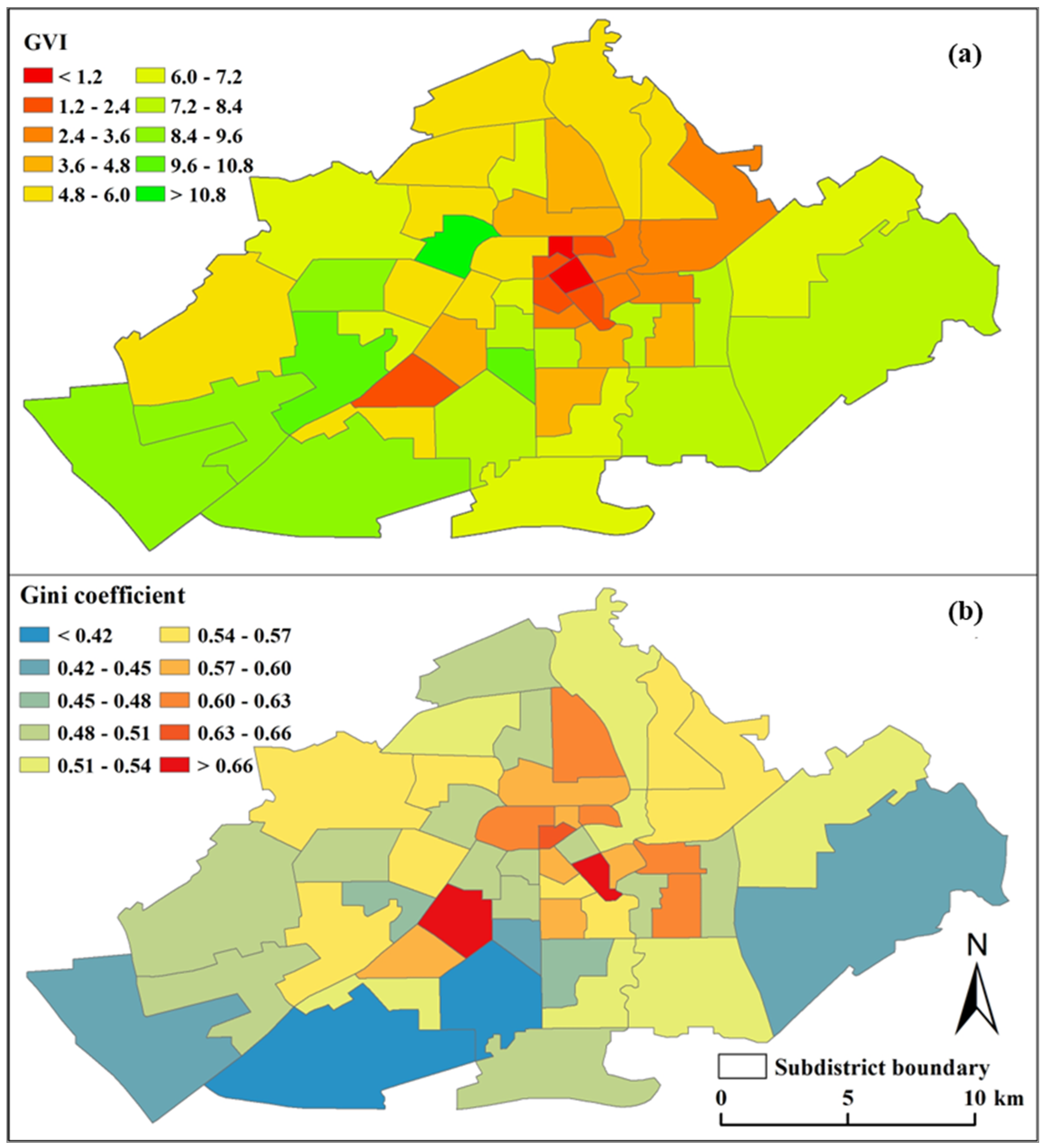
3.1. The Dispersion Patterns of the GVI and the Gini Coefficient across Space

The GVI values across the 49 subdistricts in Changchun varied from 0.40 to 10.96, with an average value of 5.50 and a standard deviation of 2.61 (Table 1). The average Gini coefficient across these 49 subdistricts was 0.53. As shown in Figure 2, the GVI in the central and northern of the city was lower than that in other areas. On the contrary, the Gini coefficient in the central and northern of the city was higher (>0.55) compared to other areas.

3.2. Description of Explanatory Variables

Table 1 shows the descriptive statistics for the three grouped explanatory variables at the subdistrict level. The GVI showed a significant positive association with housing price, PLAND, PD, LPI, ED, LSI, and AI. In contrast, the GVI showed a significant negative correlation with population density. However, no significant relationship was found between the GVI and biogeographic factors (as shown in Figure S1). The Gini coefficient showed a negative correlation with housing price, PLAND, LPI, ED, LSI, and AI (Figure S1). Conversely, a significant positive correlation was observed between the Gini coefficient and population density. However, no significant relationship was found between the Gini coefficient and biogeographic factors.

3.3. The Relative Contribution of Explanatory Variables on GVI and Gini Coefficient

The optimal BRT model accounted for 64.0% and 51.0% of the variation in the GVI and Gini coefficients, respectively (Figure 3 and Table S2). For the GVI, ED and PLAND were identified as the two most crucial drivers, contributing 41.94% and 35.36% to the explained variation, respectively. For the Gini coefficient, the three most significant driving factors were identified as PLAND, ED, and the percentage of working age. Each of these factors contributed at least 10.0% to the explained variation (Figure 3).
Landscape patterns had the highest relative influence on both GVI (88.30%) and the Gini coefficient (71.18%), while biogeographic factors had the lowest relative influence (4.65–8.12%) (Figure 3). The relative contribution of landscape patterns to the GVI was 12.5 times that of socioeconomic factors, and for the Gini coefficient, it was 3.4 times that of socioeconomic factors.

3.4. Marginal Effects of Explanatory Variables on GVI and Gini Coefficient

The GVI showed a significant increase with ED, from 200 to 286 m/ha and, with the PLAND, from 14% to 25%. A moderate positive relationship was observed between the GVI and both the LSI and housing age (Figure 4). The GVI increased with the LPI from 4% to 7%. However, the GVI exhibited a weak positive relationship with both LSI and housing age. Interestingly, the GVI did not show a significant correlation with biogeographic variables, each accounting for less than 1.75% of the variation explained (Figure 3a and Figure S2).
The Gini coefficient showed a decrease with the PLAND from 15% to 25%, after which it plateaued for PLAND values greater than or equal to 25%. When ED was less than 210 m/ha, it had no effect on the Gini coefficient. However, the Gini coefficient significantly decreased with ED from 210 to 300 m/ha (Figure 5). The Gini coefficient showed an increase with the percentage of elderly from 8% to 9.8%. Interestingly, the Gini coefficient had no significant relationship with biogeographic variables, except for building density, each accounting for less than 5.10% of the variation explained (Figure 3b and Figure S3).

4. Discussion

This study first employed Green View Index (GVI) by utilizing Baidu Street View images to quantify the availability of street greenery from the pedestrian’s perspective in a northern city of China. Compared with traditional greening metrics, which are usually based on remote sensing images, the GVI can better reflect residents’ perception of urban greenery [7,13,17]. Second, this study evaluated the fairness of the spatial distribution of street greenery quantified from the pedestrian’s perspective at the subdistrict level for the first time by using the Gini coefficient. Third, the Boosted Regression Tree (BRT) method was employed to comprehensively assess the relative importance of explanatory factors divided into socioeconomic, biogeographic, and landscape pattern factors on the availability and spatial fairness of street greenery. This process provided a new perspective for evaluating urban greening and revealing its main drivers. Most importantly, this study found that there was not a simple linear relationship between the main driving factors (e.g., PLAND and ED) and availability and spatial fairness of street greenery but a threshold effect. This finding has practical significance for urban greenery promotion and management in the future. In general, this study will provide an important reference for future urban greenery research and planning.

4.1. Availability and Spatial Fairness of Urban Street Greenery

Changchun exhibits a relatively lower average availability of street greenery compared to several cities in southern China, such as Jianghan District, Wuhan [50], and 18.80 in Kunming [51]. The GVI in Changchun is also relatively low compared to developed countries or regions such as Berkeley [16], Hartford [32], and Singapore [52]. One possible reason for this difference is that most of these cities are characterized as “Garden Cities”, known for high levels of landscaping construction and numerous green landscapes and public green spaces [31]. Another potential reason is the relatively high per capita income in these cities. Individuals with elevated earnings often dedicate more resources towards choosing or enhancing their living environments with extra greenery, thus reaping a variety of related advantages [32,53].
City centers usually have less street greenery, a finding that has been verified by an increasing number of studies in cities such as Amsterdam, Netherlands [54], Beijing [55], and Harbin, China [56]. In contrast to the suburban areas, the spatial arrangement of street greenery in the urban core is more disparate. This finding has been corroborated by studies undertaken in Beijing and Shanghai [57,58].
The results showed that the average Gini coefficient for the subdistricts in Changchun stood at 0.53, suggesting that the dispersion of street greenery, especially in the central zones of Changchun city, is relatively uneven (Figure 2). The main factors contributing to the unequal distribution of street greenery in Changchun are the limited quantity and uneven spatial distribution of green patches, particularly within city center subdistricts. Prior research has indicated that urban development has resulted in a rise in impermeable surfaces in the central region of Changchun City, leading to a diminished ratio of green areas in comparison to the peripheral regions [13,42].

4.2. The Major Factor Driving Availability and Spatial Fairness of Street Greenery

This study is the first to apply a BRT model to comprehensively analyze the effect of socioeconomic, biogeographic, and landscape patterns on the availability and spatial fairness of street greenery, as well as their relative importance. Previous research has predominantly concentrated on the impact of a single or a pair of these factors on the availability and fair dispersion of street greenery [9,13,27,59]. However, these conclusions have been indeterminate in uncovering the crucial factors influencing the availability and spatial fairness of street greenery and may not be suitable for directing urban greenery construction. The results of this study concur with prior studies, demonstrating that socioeconomic, biogeographic, and landscape patterns significantly influence street greenery. Contrary to findings from studies conducted in Western countries, this study discovered that landscape patterns, rather than socioeconomic factors, are the primary drivers of the availability and spatial fairness of street greenery (Figure 3a,b). This finding is also confirmed by research conducted in other Chinese cities [9,27,60]. One potential reason for this disparity is that in China, residential verdant areas are predominantly orchestrated and preserved by the government or property corporations, rather than dwelling owners [27,61]. In contrast, in Western countries, residential green space is exclusively used by dwelling owners. Consequently, in China, it is collectively utilized by all inhabitants of the residential sector and is thus comparatively less influenced by the financial standing of the residents.
This study found that socioeconomic factors exert a more substantial influence on then the spatial equity of street greenery than on its availability. A significant negative relationship was found between housing prices and the Gini coefficient. This implies that the spatial allocation of street greener is relatively equitable in affluent residential zones. High-income residential areas tend to show greater concern for urban green spaces resource allocation compared to low-income residential areas. For instance, many domestic real estate developers have made substantial investments in planning the greening of their properties to attract buyers [24,55]. Moreover, residents with higher socioeconomic statuses are generally more willing to invest in green construction and management [53].
This study found that PLAND and ED are the primary factors explaining the variations in the availability and spatial fairness of street greenery, which is consistent with previous studies [9,13,62]. Urban green spaces hold a pivotal function in supplying street greenery. Augmenting the ratio of these urban green zones can boost not only its availability but also its equitable dispersion. Green areas with linear and irregular forms possess extended perimeters in comparison to square configurations, thereby offering more entry points. Additionally, this study found that there is not a simple linear relationship between ED, PLAND, and the availability and equitable distribution of street greenery; instead, there exists a threshold (Figure 4 and Figure 5). Specifically, once the proportion of green space or patch complexity surpasses a certain limit, further increases do not significantly contribute to its availability and spatial fairness. This pattern may be because increasing the proportion of green space and patch shape complexity at low green cover levels can create more street greenery and enhance its spatial distribution equity. However, when green cover reaches a certain level, additional green areas become less noticeable at eye level. For example, Jiang et al. [63] found that the correlation between remotely sensed greenery and street greenery significantly decreases as green cover expands. This finding has a positive implication for guiding urban greening planning and construction. For example, this threshold can serve as guidance for planning and constructing specific areas or shapes of green spaces, thereby maximizing the improvement in availability and equitable distribution of street greenery. However, it is important to note that there are variations in planning policies, economic development, and cultural aspects among different cities. Further research involving multiple cities is necessary to determine the universality of this threshold.
While earlier research has shown a tight correlation between the dimensions of trees and the availability of street greenery [13,16,25], this study did not observe a significant correlation between these two factors at the subdistrict level (Figures S1 and S2). This discrepancy could be attributed to the uneven distribution of trees or shrubs, which may be obstructed by buildings, thereby weakening the relationship between tree size and the availability of street greenery [16,52]. Another possible explanation is that the influence of tree dimensions on the availability of street greenery may be contingent on the scale of the study. For instance, a previous study showed that as the scale increased, tree size contributed less to the variability in the availability of street greenery [13]. These findings underscore the complexity of urban greenery dynamics and the necessity for strategies tailored to the specific context in efforts to green urban areas.

4.3. Implications for Management and Policymaking

This study reveals that street greenery in the subdistricts of Changchun is relatively scant and unevenly distributed. The BRT analysis results suggest that the availability and spatial fairness of street greenery are chiefly shaped by the landscape pattern of green space, with ED and PLAND emerging as the key factors. Based on these findings, three suggestions for urban greenery construction and management in Changchun are proposed.
Firstly, the availability and spatial equity of the street greenery of Changchun can be improved by augmenting the ratio of green areas and constructing green spaces with intricate forms. While constructing large-scale green spaces is the most direct approach to increasing the proportion of green areas, it is nearly impossible to achieve this in areas with high building density. Moreover, simply expanding the greenspace area does not necessarily address the issue of unequal distribution of green spaces [8,13,64]. it is nearly impossible to achieve this in areas with high building density. Moreover, simply expanding the greenspace area does not necessarily address the issue of unequal distribution of green spaces [8,13]. For instance, most viaducts in Changchun, built to alleviate traffic congestion, provide space for urban greening. For green space shapes, linear green spaces like strips, street trees, and buffers should be considered. These types of green spaces can effectively connect overlooked and peripheral spaces within urban areas, offering a wide range of benefits, optimizing space utilization, and fostering both availability and spatial fairness of street greenery in urban environments [9,13,65].
Secondly, in future urban greenery plans, the parameters of green landscape should be considered. The BRT analysis results show that the GVI increases rapidly as both ED (286 m/ha) and PLAND (25%) increase, reaching a turning point where the rate of increase starts to decelerate. Similarly, the Gini coefficient experiences a swift decline as ED (300 m/ha) and PLAND (25%) increase before the turning point, after which the rate of decrease slows. In other words, a PLAND (proportion of green space) of 25% is ideal for optimizing both the availability and equitable spatial distribution of street greenery at the subdistrict level in Changchun. In terms of the configuration of green areas, the ideal ED (total edge/area of green patches in the subdistrict) for optimizing the availability of street greenery and the fairness of spatial distribution at the subdistrict level in Changchun stands at 286 m/ha and 300 m/ha, respectively.
Thirdly, enhancing the socioeconomic status of the residents. The study by Xiao et al. [53] suggests that residents with higher socioeconomic statuses exhibit a greater inclination to contribute to green initiatives. In other words, the issue of uneven distribution of street greenery in residential zones can be tackled by enhancing the socioeconomic status of residents. However, as we know, improving residents’ socioeconomic status is a complex and long-term project, and it is challenging to address the uneven distribution of green spaces solely by increasing residents’ income in a short time. Therefore, currently, the best approach to enhance the spatial equity of urban street greenery is through the regulation of green space landscape patterns.

4.4. Limitations and Future Studies

Despite this study making considerable progress in quantifying the availability and spatial fairness of street greenery at the subdistrict level and analyzing their primary influencing factors, there remain limitations that upcoming studies need to tackle. Firstly, this study used the GVI to access the street greenery based on BSV images. The original BSV image data, sourced from static images captured along the streets, could be affected by vehicles and other obstructions along the streets [66]. The calculated GVI values could be influenced by this, which in turn could affect subsequent analyses that rely on these values. To reduce this uncertainty, it is recommended that future research should contemplate the integration of various data sources [67]. Secondly, the focus of this study was to examine the influence of socioeconomic elements, biogeographic variables, and landscape patterns on the street greenery. However, street greenery may also be influenced by other factors such as urban microclimate and the impact of management measures [31,41,68]. To comprehensively reveal the driving factors and mechanisms of street greenery, future research should consider the influence of these factors. Third, this study found that some driving factors exhibit a threshold effect on street greenery. Whether this pattern is universal or not requires further research across multiple cities for validation.

5. Conclusions

This study introduces an innovative approach by using the GVI and Gini coefficient to quantify the availability and spatial fairness of street greenery based on BSV images. This offers a more detailed perspective than traditional aerial perspective assessments. Additionally, this study presents a new framework for urban greening research. The results reveal that the availability of street greenery in Changchun is relatively scant and unevenly distributed. Urban centers have lower availability and spatial fairness of street greenery compared to suburban areas. The availability and spatial fairness of street greenery are primarily driven by the patterns of green space landscape. ED and PLAND emerge as the two most important factors, showing a threshold effect on the availability and spatial fairness of street greenery. Increasing the proportion of green space and creating complex-shaped green spaces can effectively improve street greenery availability and spatial fairness. The optimal PLAND for improving the availability of street greenery and its spatial fairness is 25%, while the optimal ED is 286 m/ha and 300 m/ha, respectively. This study offers a new viewpoint for future planning and management of urban greening.

Supplementary Materials

The following supporting information can be downloaded at: https://www.mdpi.com/article/10.3390/f15071074/s1, Figure S1: Bivariate relationships between variables used in this study. Right upper: pairwise comparisons of 21 predictors factors of GVI and Gini coefficient are shown, with a color gradient denoting the Spearman’s correlation coefficients; left bottom: edge width corresponds to the Pearson’s correlations coefficient and edge color denotes the statistical significance; Figure S2: Partial dependence plots showing the marginal relationship between GVI and each predictor while accounting for the average effects of the other predictors in BRT analysis; Figure S3: Partial dependence plots showing the marginal relationship between Gini coefficient and each predictor while accounting for the average effects of the other predictors in BRT analysis; Table S1: The number of Baidu Street View-generating points and survey samples in each subdistrict; Table S2: List of landscape metrics and their descriptions (McGarigal et al., 2023 [69]); Table S3: Model selection of boosted regression tree analyses (BRT) of GVI and Gini coefficient. The PE percentage changes were used to determine the optimal BRT model from models with TC values from 1 to 6. Trees, R2, and PE showed the average value of the 30 replicates of BRT models for both GVI and Gini coefficients; Table S4: Moran’s I statistics of the residuals of the BRT analysis of GVI and Gini coefficient. The significance of the Moran’s I statistic at each distance class was obtained by using the permutation test. These analyses were conducted in SAM v4.0.

Author Contributions

L.X. conceived the ideas. L.X. and W.W. designed the methodology and supervised the study. L.X. wrote the original draft of the manuscript. W.W., Z.R., C.W. and X.H. reviewed and edited the manuscript. All authors have read and agreed to the published version of the manuscript.

Funding

This study was supported by the National Natural Science Foundation of China (32201441, 31670699), Fundamental Research Funds for the Central Universities (2572017DG04), and the Longjiang Professor Fund from Northeast Forestry University.

Data Availability Statement

Data will be made available on request.

Conflicts of Interest

The authors declare no competing interests.

References

  1. Rizwan, A.M.; Dennis, L.Y.; Chunho, L. A review on the generation, determination and mitigation of Urban Heat Island. J. Environ. Sci. 2008, 20, 120–128. [Google Scholar] [CrossRef]
  2. Wang, W.; Tian, P.; Zhang, J.; Agathokleous, E.; Xiao, L.; Koike, T.; Wang, H.; He, X. Big data-based urban greenness in Chinese megalopolises and possible contribution to air quality control. Sci. Total Environ. 2022, 824, 153834. [Google Scholar] [CrossRef]
  3. Song, Y.; Chen, B.; Ho, H.C.; Kwan, M.-P.; Liu, D.; Wang, F.; Wang, J.; Cai, J.; Li, X.; Xu, Y.; et al. Observed inequality in urban greenspace exposure in China. Environ. Int. 2021, 156, 106778. [Google Scholar] [CrossRef]
  4. Miao, C.; Yu, S.; Hu, Y.; Liu, M.; Yao, J.; Zhang, Y.; He, X.; Chen, W. Seasonal effects of street trees on particulate matter concentration in an urban street canyon. Sustain. Cities Soc. 2021, 73, 103095. [Google Scholar] [CrossRef]
  5. Chan, S.H.M.; Qiu, L.; Esposito, G.; Mai, K.P. Vertical greenery buffers against stress: Evidence from psychophysiological responses in virtual reality. Landsc. Urban Plan. 2021, 213, 104127. [Google Scholar] [CrossRef]
  6. Cheng, Y.; Zhang, J.; Wei, W.; Zhao, B. Effects of urban parks on residents’ expressed happiness before and during the COVID-19 pandemic. Landsc. Urban Plan. 2021, 212, 104118. [Google Scholar] [CrossRef]
  7. Helbich, M.; Yao, Y.; Liu, Y.; Zhang, J.; Liu, P.; Wang, R. Using deep learning to examine street view green and blue spaces and their associations with geriatric depression in Beijing, China. Environ. Int. 2019, 126, 107–117. [Google Scholar] [CrossRef]
  8. Wolch, J.R.; Byrne, J.; Newell, J.P. Urban green space, public health, and environmental justice: The challenge of making cities ‘just green enough’. Landsc. Urban Plan. 2014, 125, 234–244. [Google Scholar] [CrossRef]
  9. Guan, J.; Wang, R.; Van Berkel, D.; Liang, Z. How spatial patterns affect urban green space equity at different equity levels: A Bayesian quantile regression approach. Landsc. Urban Plan. 2023, 233, 104709. [Google Scholar] [CrossRef]
  10. Yang, G.; Zhao, Y.; Xing, H.; Fu, Y.; Liu, G.; Kang, X.; Mai, X. Understanding the changes in spatial fairness of urban greenery using time-series remote sensing images: A case study of Guangdong-Hong Kong-Macao Greater Bay. Sci. Total Environ. 2020, 715, 136763. [Google Scholar] [CrossRef] [PubMed]
  11. Dobbs, C.; Nitschke, C.; Kendal, D. Assessing the drivers shaping global patterns of urban vegetation landscape structure. Sci. Total Environ. 2017, 592, 171–177. [Google Scholar] [CrossRef]
  12. Schule, S.A.; Gabriel, K.M.A.; Bolte, G. Relationship between neighbourhood socioeconomic position and neighbourhood public green space availability: An environmental inequality analysis in a large German city applying generalized linear models. Int. J. Hyg. Environ. Health 2017, 220, 711–718. [Google Scholar] [CrossRef]
  13. Xiao, L.; Wang, W.; Ren, Z.; Fu, Y.; Lv, H.; He, X. Two-city street-view greenery variations and association with forest attributes and landscape metrics in NE China. Landsc. Ecol. 2021, 36, 1261–1280. [Google Scholar] [CrossRef]
  14. Lu, Y.; Sarkar, C.; Xiao, Y. The effect of street-level greenery on walking behavior: Evidence from Hong Kong. Soc. Sci. Med. 2018, 208, 41–49. [Google Scholar] [CrossRef]
  15. Li, X.; Zhang, C.; Li, W.; Ricard, R.; Meng, Q.; Zhang, W. Assessing street-level urban greenery using Google Street View and a modified green view index. Urban For. Urban Green. 2015, 14, 675–685. [Google Scholar] [CrossRef]
  16. Yang, J.; Zhao, L.; McBride, J.; Gong, P. Can you see green? Assessing the visibility of urban forests in cities. Landsc. Urban Plan. 2009, 91, 97–104. [Google Scholar] [CrossRef]
  17. Li, X.; Ghosh, D. Associations between Body Mass Index and Urban “Green” Streetscape in Cleveland, Ohio, USA. Int. J. Environ. Res. Public Health 2018, 15, 2186. [Google Scholar] [CrossRef]
  18. Nesbitt, L.; Meitner, M.J.; Girling, C.; Sheppard, S.R.J.; Lu, Y. Who has access to urban vegetation? A spatial analysis of distributional green equity in 10 US cities. Landsc. Urban Plan. 2019, 181, 51–79. [Google Scholar] [CrossRef]
  19. Pearsall, H.; Eller, J.K. Locating the green space paradox: A study of gentrification and public green space accessibility in Philadelphia, Pennsylvania. Landsc. Urban Plan. 2020, 195, 103708. [Google Scholar] [CrossRef]
  20. Halecki, W.; Stachura, T.; Fudała, W.; Stec, A.; Kuboń, S. Assessment and planning of green spaces in urban parks: A review. Sustain. Cities Soc. 2022, 88, 104280. [Google Scholar] [CrossRef]
  21. Yu, Z.; Ma, W.; Hu, S.; Yao, X.; Yang, G.; Yu, Z.; Jiang, B. A simple but actionable metric for assessing inequity in resident greenspace exposure. Ecol. Indic. 2023, 153, 110423. [Google Scholar] [CrossRef]
  22. Hope, D.; Gries, C.; Zhu, W.; Fagan, W.F.; Redman, C.L.; Grimm, N.B.; Nelson, A.L.; Martin, C.; Kinzig, A. Socioeconomics drive urban plant diversity. Proc. Natl. Acad. Sci. USA 2003, 100, 8788–8792. [Google Scholar] [CrossRef]
  23. Kabisch, N.; Haase, D. Green justice or just green? Provision of urban green spaces in Berlin, Germany. Landsc. Urban Plan. 2014, 122, 129–139. [Google Scholar] [CrossRef]
  24. Wang, H.; Qiu, J.; Breuste, J.; Friedman, C.R.; Zhou, W.; Wang, X. Variations of urban greenness across urban structural units in Beijing, China. Urban For. Urban Green. 2013, 12, 554–561. [Google Scholar] [CrossRef]
  25. Chen, Z.; Xu, B.; Gao, B. Assessing visual green effects of individual urban trees using airborne Lidar data. Sci. Total Environ. 2015, 536, 232–244. [Google Scholar] [CrossRef]
  26. Gong, F.; Zeng, Z.; Zhang, F.; Li, X.; Ng, E.; Norford, L.K. Mapping sky, tree, and building view factors of street canyons in a high-density urban environment. Build. Environ. 2018, 134, 155–167. [Google Scholar] [CrossRef]
  27. Hu, L.; Fan, C.; Cai, Z.; Liao, W.; Li, X. Greening residential quarters in China: What are the roles of urban form, socioeconomic factors, and biophysical context? Urban For. Urban Green. 2023, 86, 128020. [Google Scholar] [CrossRef]
  28. Ren, Z.; Zheng, H.; He, X.; Zhang, D.; Shen, G.; Zhai, C. Changes in spatio-temporal patterns of urban forest and its above-ground carbon storage: Implication for urban CO2 emissions mitigation under China’s rapid urban expansion and greening. Environ. Int. 2019, 129, 438–450. [Google Scholar] [CrossRef]
  29. Jin, Y.; Chen, G.; Ma, W. Pre-recognition of the Target Orientation of the ‘National Garden City’ from the Evolution of Evaluation Indexes. Shanghai Urban Planning 2015, 5, 75–80. [Google Scholar]
  30. Shen, Y.; Sun, F.; Che, Y. Public green spaces and human wellbeing: Mapping the spatial inequity and mismatching status of public green space in the Central City of Shanghai. Urban For. Urban Green. 2017, 27, 59–68. [Google Scholar] [CrossRef]
  31. Long, Y.; Liu, L. How green are the streets? An analysis for central areas of Chinese cities using Tencent Street View. PLoS ONE 2017, 12, e0171110. [Google Scholar] [CrossRef]
  32. Li, X.; Zhang, C.; Li, W.; Kuzovkina, Y.A.; Weiner, D. Who lives in greener neighborhoods? The distribution of street greenery and its association with residents’ socioeconomic conditions in Hartford, Connecticut, USA. Urban For. Urban Green. 2015, 14, 751–759. [Google Scholar] [CrossRef]
  33. Cowell, F. Measuring Inequality, 3rd ed.; Oxford University Press: Oxford, UK, 2010. [Google Scholar]
  34. Boyce, J.K.; Zwickl, K.; Ash, M. Measuring environmental inequality. Ecol. Econ. 2016, 124, 114–123. [Google Scholar] [CrossRef]
  35. Yao, L.; Liu, J.; Wang, R.; Yin, K.; Han, B. Effective green equivalent—A measure of public green spaces for cities. Ecol. Indic. 2014, 47, 123–127. [Google Scholar] [CrossRef]
  36. Han, Y.; He, J.; Liu, D.; Zhao, H.; Huang, J. Inequality in urban green provision: A comparative study of large cities throughout the world. Sustain. Cities Soc. 2023, 89, 104229. [Google Scholar] [CrossRef]
  37. Zhu, Z.; Pei, H.; Schamp, B.S.; Qiu, J.; Cai, G.; Cheng, X.; Wang, H. Land cover and plant diversity in tropical coastal urban Haikou, China. Urban For. Urban Green. 2019, 44, 126395. [Google Scholar] [CrossRef]
  38. Wang, H.F.; Qureshi, S.; Knapp, S.; Friedman, C.R.; Hubacek, K. A basic assessment of residential plant diversity and its ecosystem services and disservices in Beijing, China. Appl. Geogr. 2015, 64, 121–131. [Google Scholar] [CrossRef]
  39. Guo, J.; Fang, Y.; Zhu, B. Study of selection in price-earnings ratio indication factors. J. Anhui Agric. Sci. 2007, 35, e5968. [Google Scholar]
  40. Wang, W.; Xiao, L.; Zhang, J.; Yang, Y.; Tian, P.; Wang, H.; He, X. Potential of Internet street-view images for measuring tree sizes in roadside forests. Urban For. Urban Green. 2018, 35, 211–220. [Google Scholar] [CrossRef]
  41. Ren, Z.; Zheng, H.; He, X.; Zhang, D.; Yu, X. Estimation of the Relationship Between Urban Vegetation Configuration and Land Surface Temperature with Remote Sensing. J. Indian Soc. Remote Sens. 2015, 43, 89–100. [Google Scholar]
  42. Zhang, D.; Wang, W.; Zheng, H.; Ren, Z.; Zhai, C.; Tang, Z.; Shen, G.; He, X. Effects of urbanization intensity on forest structural-taxonomic attributes, landscape patterns and their associations in Changchun, Northeast China: Implications for urban green infrastructure planning. Ecol. Indic. 2017, 80, 286–296. [Google Scholar] [CrossRef]
  43. R Core Team. R: A Language and Environment for Statistical Computing; R Core Team: Vienna, Austria, 2013. [Google Scholar]
  44. Elith, J.; Leathwick, J.R.; Hastie, T. A working guide to boosted regression trees. J. Anim. Ecol. 2008, 77, 802–813. [Google Scholar] [CrossRef]
  45. Yan, H.F.; Kyne, P.M.; Jabado, R.W.; Leeney, R.H.; Davidson, L.N.K.; Derrick, D.H.; Finucci, B.; Freckleton, R.P.; Fordham, S.V.; Dulvy, N.K. Overfishing and habitat loss drives range contraction of iconic marine fishes to near extinction. Sci. Adv. 2021, 7, eabb6026. [Google Scholar] [CrossRef]
  46. Yuan, Z.; Ali, A.; Wang, S.; Gazol, A.; Freckleton, R.; Wang, X.; Lin, F.; Ye, J.; Zhou, L.; Hao, Z.; et al. Abiotic and biotic determinants of coarse woody productivity in temperate mixed forests. Sci. Total Environ. 2018, 630, 422–431. [Google Scholar] [CrossRef] [PubMed]
  47. Lin, D.; Anderson-Teixeira, K.J.; Lai, J.; Mi, X.; Ren, H.; Ma, K. Traits of dominant tree species predict local scale variation in forest aboveground and topsoil carbon stocks. Plant Soil 2016, 409, 435–446. [Google Scholar] [CrossRef]
  48. Jim, C.Y.; Chen, W.Y. Impacts of urban environmental elements on residential housing prices in Guangzhou (China). Landsc. Urban Plan. 2006, 78, 422–434. [Google Scholar] [CrossRef]
  49. Lutzenhiser, M.; Netusil, N.R. The effect of open spaces on a home’s sale price. Contemp. Econ. Policy 2001, 19, 291–298. [Google Scholar] [CrossRef]
  50. Chen, M.; Dai, F.; Li, W.; Yang, C. A Study of Urban Greening Assessment Based on Visible Green Index: A Case Study of Jianghan District in Wuhan. J. Chin. Urban For. 2019, 17, 1–6. [Google Scholar]
  51. Yang, Y. Research on Green Looking Ratio and Scenic Beauty Estimation on Business District in Main Urban Area in Kunming; Southwest Forestry University Kunming: Kunming, China, 2017. [Google Scholar]
  52. Ye, Y.; Richards, D.; Lu, Y.; Song, X.; Zhuang, Y.; Zeng, W.; Zhong, T. Measuring daily accessed street greenery: A human-scale approach for informing better urban planning practices. Landsc. Urban Plan. 2019, 191, 103434. [Google Scholar] [CrossRef]
  53. Xiao, Y.; Lu, Y.; Guo, Y.; Yuan, Y. Estimating the willingness to pay for green space services in Shanghai: Implications for social equity in urban China. Urban For. Urban Green. 2017, 26, 95–103. [Google Scholar] [CrossRef]
  54. Elenbaas, H. Amsterdam and the Spatial Justice Debate: Studying the Distributional Equality of Urban Greenery; University of Utrecht: Utrecht, The Netherlands, 2018. [Google Scholar]
  55. Zhang, Y.; Dong, R. Impacts of Street-Visible Greenery on Housing Prices: Evidence from a Hedonic Price Model and a Massive Street View Image Dataset in Beijing. ISPRS Int. J. Geo-Inf. 2018, 7, 104. [Google Scholar] [CrossRef]
  56. Lv, H.; Wang, W.; He, X.; Wei, C.; Xiao, L.; Zhang, B.; Zhou, W. Association of urban forest landscape characteristics with biomass and soil carbon stocks in Harbin City, Northeastern China. PeerJ 2018, 6, e5825. [Google Scholar] [CrossRef] [PubMed]
  57. Guo, S.; Song, C.; Pei, T.; Liu, Y.; Ma, T.; Du, Y.; Chen, J.; Fan, Z.; Tang, X.; Peng, Y. Accessibility to urban parks for elderly residents: Perspectives from mobile phone data. Landsc. Urban Plan. 2019, 191, 103642. [Google Scholar] [CrossRef]
  58. Fan, P.; Xu, L.; Yue, W.; Chen, J. Accessibility of public urban green space in an urban periphery: The case of Shanghai. Landsc. Urban Plan. 2017, 165, 177–192. [Google Scholar] [CrossRef]
  59. Łaszkiewicz, E.; Wolff, M.; Andersson, E.; Kronenberg, J.; Barton, D.N.; Haase, D.; Langemeyer, J.; Baró, F.; McPhearson, T. Greenery in urban morphology: A comparative analysis of differences in urban green space accessibility for various urban structures across European cities. Ecol. Soc. 2022, 27, 22. [Google Scholar] [CrossRef]
  60. Wang, H.-F.; Qureshi, S.; Qureshi, B.A.; Qiu, J.-X.; Friedman, C.R.; Breuste, J.; Wang, X.-K. A multivariate analysis integrating ecological, socioeconomic and physical characteristics to investigate urban forest cover and plant diversity in Beijing, China. Ecol. Indic. 2016, 60, 921–929. [Google Scholar] [CrossRef]
  61. Yan, J.; Zhou, W.; Zheng, Z.; Wang, J.; Tian, Y. Characterizing variations of greenspace landscapes in relation to neighborhood characteristics in urban residential area of Beijing, China. Landsc. Ecol. 2020, 35, 203–222. [Google Scholar] [CrossRef]
  62. Ngom, R.; Gosselin, P.; Blais, C. Reduction of disparities in access to green spaces: Their geographic insertion and recreational functions matter. Appl. Geogr. 2016, 66, 35–51. [Google Scholar] [CrossRef]
  63. Jiang, B.; Deal, B.; Pan, H.; Larsen, L.; Hsieh, C.-H.; Chang, C.-Y.; Sullivan, W.C. Remotely-sensed imagery vs. eye-level photography: Evaluating associations among measurements of tree cover density. Landsc. Urban Plan. 2017, 157, 270–281. [Google Scholar] [CrossRef]
  64. Pietilä, M.; Neuvonen, M.; Borodulin, K.; Korpela, K.; Sievänen, T.; Tyrväinen, L. Relationships between exposure to urban green spaces, physical activity and self-rated health. J. Outdoor Recreat. Tour. 2015, 10, 44–54. [Google Scholar] [CrossRef]
  65. Yang, Y.; Lu, Y.; Yang, H.; Yang, L.; Gou, Z. Impact of the quality and quantity of eye-level greenery on park usage. Urban For. Urban Green. 2021, 60, 127061. [Google Scholar] [CrossRef]
  66. Baidu. Web Services API. Available online: http://lbsyun.baidu.com/ (accessed on 20 May 2019).
  67. Li, X. Examining the spatial distribution and temporal change of the green view index in New York City using Google Street View images and deep learning. Environ. Plan. B-Urban 2020, 48, 2039–2054. [Google Scholar] [CrossRef]
  68. Wu, S.; Chen, B.; Webster, C.; Xu, B.; Gong, P. Improved human greenspace exposure equality during 21(st) century urbanization. Nat. Commun. 2023, 14, 6460. [Google Scholar] [CrossRef]
  69. McGarigal, K.; Cushman S., A.; Ene, E. FRAGSTATS v4: Spatial Pattern Analysis Program for Categorical Maps. 2023. Available online: http://www.fragstats.org/ (accessed on 1 December 2023).
Figure 1. Study area locations and sampling points.
Forests 15 01074 g001
Figure 2. The spatial distribution of both the GVI (a) and the Gini coefficient (b) at the subdistrict level within the study area.
Forests 15 01074 g002
Figure 3. The relative importance of socioeconomic, biogeographic, and landscape pattern factors explained the variation between the GVI (a) and Gini coefficient (b). Pie charts show the summed relative importance of socioeconomic, biogeographic, and landscape pattern factors. The error bars represent the 95% confidence intervals, which are derived from 1000 bootstrap samples of the original dataset consisting of 30 entries. The abbreviations of variables are provided in Table 1.
Forests 15 01074 g003
Figure 4. Partial dependence plots for explanatory variables for GVI. Only the significant relationships are displayed (refer to Figure S2 for additional information). Each gray dot represents the observed value for a single subdistrict. The abbreviations of variables are provided in Table 1.
Forests 15 01074 g004
Figure 5. Partial dependence plots for explanatory variables for Gini coefficient. Only the significant relationships are displayed (refer to Figure S3 for additional information). Each gray dot represents the observed value for a single subdistrict. The abbreviations of variables are provided in Table 1.
Forests 15 01074 g005
Table 1. Descriptive statistics of GVI, Gini coefficient, and explanatory variables.
VariablesMeanRangeStd. Dev.
GVI5.50.4–10.962.61
Gini coefficient0.530.4–0.670.06
Socioeconomic factors
Population density (persons/km2)18,073.87714.43–43,830.2011,851.64
Percentage of youth (%)9.615.96–15.472.07
Percentage of working age (%)81.5276.48–90.962.55
Percentage of elderly (%)8.873.08–15.232.45
Percentage of permanent residents (%)62.2221.42–92.3314.99
Housing price (103 yuan/m2)9.376.63–14.851326.93
Housing age (years)15.842.00–92.0025.91
Biogeographic factors
Building density (%)20.928.00–35.000.07
Road density (km/km2)6.572.08–14.802.94
Floor area ratio (FAR)0.930.25–2.280.45
Elevation (m)209.83182.08–241.0413.95
Diameter at breast height (DBH, cm)20.8413.43–37.136.12
Tree height (TH, m)8.275.43–11.721.51
Height under branch of tree (UBH, cm)280.21163.85–453.0856.76
Canopy size (CS, cm)494.68311.28–852.58160.63
Landscape pattern
Percentage of landscape (PLAND, %)22.241.42–52.1211.50
Patch density (PD, number/100 ha)95.6625.36–147.1229.01
Large patch index (LPI, %)6.460.19–30.226.42
Edge Density (ED, m/ha)238.114.60–368.5978.62
Landscape shape index (LSI)30.254.41–74.4314.98
Aggregation Index (AI, %)93.6585.66–97.762.42
Disclaimer/Publisher’s Note: The statements, opinions and data contained in all publications are solely those of the individual author(s) and contributor(s) and not of MDPI and/or the editor(s). MDPI and/or the editor(s) disclaim responsibility for any injury to people or property resulting from any ideas, methods, instructions or products referred to in the content.

