Forest Wildfire Detection from Images Captured by Drones Using Window Transformer without Shift

Abstract

Cameras, especially those carried by drones, are the main tools used to detect wildfires in forests because cameras have much longer detection ranges than smoke sensors. Currently, deep learning is main method used for fire detection in images, and Transformer is the best algorithm. Swin Transformer restricts the computation to a fixed-size window, which reduces the amount of computation to a certain extent, but to allow pixel communication between windows, it adopts a shift window approach. Therefore, Swin Transformer requires multiple shifts to extend the receptive field to the entire image. This somewhat limits the network’s ability to capture global features at different scales. To solve this problem, instead of using the shift window method to allow pixel communication between windows, we downsample the feature map to the window size after capturing global features through a single Transformer, and we upsample the feature map to the original size and add it to the previous feature map. This way, there is no need for multiple layers of stacked window Transformers; global features are captured after each window Transformer operation. We conducted experiments on the Corsican fire dataset captured by ground cameras and on the Flame dataset captured by drone cameras. The results show that our algorithm performs the best. On the Corsican fire dataset, the mIoU, F1 score, and OA reached 79.4%, 76.6%, and 96.9%, respectively. On the Flame dataset, the mIoU, F1 score, and OA reached 84.4%, 81.6%, and 99.9%, respectively.

1. Introduction

Fire is currently one of the most common and widespread major disasters that threaten the security and development of societies, and statistics from the European Forest Fire Information System (EFFIS) show that in 2021, forest fires covered 4260 hectares in Spain, more than 150,000 hectares in Italy, and 93,600 hectares in Greece [1,2,3]. To mitigate the risks associated with fires, people have proposed numerous detection methods to minimize the damage caused by such accidents. These fire detection approaches can be broadly categorized into traditional fire alarm systems and visual sensor-based detection methods.

Traditional fire alarm detection systems commonly use sensors such as smoke, heat, and light detectors to detect fires. However, these systems often require human intervention to confirm fire information when triggering alarms. Due to the rapid spread and destructive nature of fires, as well as factors such as distance, affecting sensor performance, there can be delays in detection, leading to missed opportunities for early suppression [4,5,6]. To overcome these limitations, researchers have explored several visual sensor-based detection methods. Initially, techniques were widely used to distinguish fire from the background and identify fire pixels. Various color spaces, including HSI (Hue, Saturation, Intensity) [7], YCbCr [8], and RGB (Red, Green, Blue) [9,10] have been utilized to represent fire pixels. However, these methods often struggle with accurately in detecting fire because they are highly sensitive to changes in lighting and it is challenging to precisely define the color range of fire pixels. To address these limitations, researchers have explored more robust vision-based approaches, which not only consider color but also incorporate additional features like texture and motion. Despite these advancements, one of the major challenges faced by vision-based detection methods is precisely identifying and analyzing the leading edge of surface fires, which denotes the boundary where the fire propagates across the ground [11] due to the irregular shape, size, and complex background interference [12]. In the early stages, Qiu et al. [13] proposed a novel algorithm to clearly and continuously define the edges of flames and fire points. Experimental results obtained in the laboratory using various flame images and video frames demonstrated the effectiveness and robustness of the algorithm. However, further evaluation of the algorithm’s performance in real-life fire detection scenarios was not conducted. Chino et al. [14] introduced “BoWFire” (Best of Both Worlds Fire detection), a method for fire detection that merges color and texture features to minimize false positives [15]. Similarly, Jamali et al. [16] utilized this combination of color and texture features to detect fire. Celik et al. [17] proposed a real-time fire detector that combines foreground object information with statistical information on colored fire pixels. They then refined the classification of fire pixels using a general statistical model, achieving a final correct detection rate of 98.89%. Byoung et al. [18] employed fuzzy finite automaton based on visual feature probability density functions to detect fire and non-fire videos. Their method outperformed other approaches tested in the experiment in terms of performance.

With the development of artificial intelligence in the field of computer vision, deep learning [19] became a mainstream approach as soon as it appeared, with the advantage of automatically extracting the required features, and it has been used to analyze and extract information from images taken by drones [20,21,22,23,24], autonomous vehicles [25], pedestrian detectors [26], and video surveillance equipment [27,28]. In 1998, Lecun first introduced LeNet [29], which utilizes convolutional neural networks (CNNs). LeNet employs weight sharing to reduce the computational burden of neural networks, significantly advancing the application of deep learning in image recognition. Gonzalez et al. [30] introduced the SFEwANSD (Simple Feature Extraction with FCN AlexNet, Single Deconvolution) technique for monitoring fires using UAVs (Unmanned Aerial Vehicles). This method utilizes two convolutional neural networks, namely AlexNet [31] and a basic CNN, to effectively identify fire features. Muhammad et al. [32] proposed an energy-efficient CNN approach using the SqueezeNet [33] model for fire detection and localization in closed-circuit television (CCTV) networks. However, CNNs have their limitations. During the backpropagation process, they often suffer from slow parameter updates, convergence to local optima, information loss in pooling layers, and unclear interpretation of feature extraction, among other issues. The Transformer model [34], initially proposed by the Google team in 2017, replaces the convolutional neural network components with self-attention modules. This model adopts multiple attention heads to process and capture different input data features, thereby enhancing feature extraction capabilities. However, Transformer has a high level of computational complexity in image processing. Therefore, the Microsoft team proposed Swin Transformer [35], which divides the image into multiple uniformly sized windows and limits the computation of Transformer within the windows to reduce computational load. As the depth and complexity of models have increased, segmentation accuracy has comprehensively surpassed that of traditional methods such as machine learning to become mainstream. Many scholars have applied deep learning methods to fire detection, and various deep learning models have been applied to tasks in different fields. Jadon et al. [36] constructed a lightweight neural network, FireNet, which occupies only 7.45M of disk space, and deployed it on Raspberry Pi 3B [37] embedded devices to replace conventional physical sensors. It can stably operate at a frame rate of 24 frames per second and achieved an accuracy of over 93% on experimental datasets.

Although significant achievements have been made in fire detection using deep learning technology, there still exists a considerable gap in wildfire image segmentation [20]. Compared to traditional fire detection, wildfire image segmentation techniques can provide more detailed fire information, including fire scale, flame-spreading speed, and precise fire location. This information is crucial for formulating effective prevention and control strategies and rational allocation of firefighting resources. Wang et al. [38] combined an adaptive multi-scale attention mechanism and focal loss function based on Swin Transformer to segment forest fire images, achieving an IoU of 86.73%. This is a significant improvement compared to traditional models such as PSPNet [39], SegNet [40], DeepLabV3 [41], and FCN [42]. Bochkov et al. [43] introduced wUUNet, an advanced U-Net variant with extended skip connections. It uses a two-step process. The first U-Net detects fire regions, and the second refines this result by segmenting fire colors like orange, red, and yellow.

Many scholars have also modified the YOLO series for flame recognition. Xue et al. [44] modified the original Spatial Pyramid Pooling-Fast (SPPF) module in YOLOv5 to a Spatial Pyramid Pooling-Fast-Plus (SPPFP) module for fire detection. They observed a 10.1% improvement in [email protected] on their dataset. Zhu et al. [45] used an improved YOLOv7-tiny [46] model to detect cabin fires, achieving a 2.6% increase in [email protected] and a 10 fps speed improvement. Hojune Ann et al. [47] developed a proactive fire risk detection system that performs object detection on images captured by surveillance cameras to determine whether both a fire source and combustible materials are present. The performance of two deep learning models, namely YOLOv5 [48] and EfficientDet, was compared. Kuldoshbay Avazov et al. [49] developed a novel convolutional neural network using an enhanced YOLOv4 [50] to detect fire areas. Experiments demonstrated that the proposed method can successfully be used for urban fire monitoring. Soon-Young Kim et al. [51] proposed an improved version of the YOLOv7 model, successfully detecting smoke from forest fires with an AP50 of 86.4%, which is 3.9% higher than previous single-stage and multi-stage object detectors.

Many scholars have utilized various CNNs or Swin Transformer networks for fire detection. CNNs can only capture local features; to capture global features, layer stacking is required. Similarly, Swin Transformer limits computations within windows and confines receptive fields within these windows. Consequently, Swin Transformer also requires layer stacking to expand receptive fields to cover the entire image. Moreover, in layers with large feature map sizes, Swin Transformer’s global feature-capturing ability is weak, diminishing the effectiveness of step-by-step decoding. Therefore, the main focus of this research is to address the issue of Swin Transformer’s window interactions being limited to adjacent windows and how to more efficiently integrate global and local features. The innovations of this paper are summarized as follows:

(1) We propose a non shift window Transformer module. Unlike Swin Transformer, which requires layer stacking to gradually expand the receptive field to cover the entire image, our method ensures that after each window Transformer operation, all pixels capture global features. This enhances the global feature-capturing capability of shallow layers of the network and strengthens the effectiveness of step-by-step decoding.

(2) We propose a network that integrates local and global features, where local features are captured using CNNs and global features are captured using non-shift window Transformer modules. These features are effectively fused in the network.

(3) We conducted experiments on a ground camera dataset and a drone camera dataset to analyze the generalization ability of the individual networks.

2. Study Dataset

2.1. The Corsican Fire Dataset

The Corsican Fire Dataset [52] is located at 42°7′ north latitude and 9°0′ east longitude, haute-Corse, Corsica, France. It is produced by the “Environmental Science UMR CNRS 6134 SPE” laboratory at the University of Corsica. The Corsican Fire Dataset, after removing near-infrared images, consists of 1135 images with masks depicting fire. We utilized all of these images as the training set. Since all images in the Corsican Fire Dataset depict fire, training a model to distinguish objects similar to fire from actual fire becomes challenging. Therefore, we included 36 images without fire from the BoWFire Dataset [14] in the training set, while the remaining 71 non-fire images from the BoWFire Dataset, along with the 119 fire images, formed the test set. This resulted in a training set comprising 1171 images, including images with and without fire, and a test set comprising 190 images, also including images with and without fire. All images and their corresponding masks were cropped to 256 × 256 pixels. The images were converted to JPG format, while the masks were converted to PNG format, where pixels representing fire were labeled as 1, and pixels representing no fire were labeled as 0.

2.2. The Flame Dataset

The Flame Dataset [53] is a forest fire detection dataset captured by drones during a prescribed pile burn in Northern Arizona, USA. it is published by scholars from the University of Northern Arizona and other institutions. There are a total of 2003 images with a mask, so 1800 images were used as the training set, and 203 images were used as the testing set. Due to the close similarity of all image contents, 107 non-fire images such as sunsets and lighting from the BoWFire dataset were also added to the dataset. Of these, 73 were added to the training set, while the remaining 34 images were added to the testing set. Therefore, there were a total of 1873 images in the training set and 237 images in the test set. The resolution of Flame dataset images is 3480 × 2160, so they were to 256 × 256 pixels for model processing. The images were converted to JPG format, while the masks were converted to PNG format, where pixels representing fire were labeled as 1, and pixels representing no fire were labeled as 0.

3. Method

3.1. Nswin Transformer

In processing images, transformers require significant computational overhead. To mitigate this, Liu from Microsoft Research Asia proposed Swin Transformer. Swin Transformer divides the image into several equally sized windows, constraining computations for each pixel to the pixels within its window, as illustrated in Figure 1.

Figure 1b shows the ViT method, where the entire image undergoes Transformer operations together. In contrast, Figure 1a depicts the Swin Transformer approach, where the image is divided into several equally sized patches according to the window size. Swin Transformer confines pixel computations to within the same window, hindering pixel interaction between windows. To address this, Swin Transformer employs a shifting-window mechanism, where windows are simultaneously shifted rightward and downward by half of the window width, ensuring different pixel coverage within each window, as shown in Figure 2. By alternating stacking between window Transformer and window-shifting Transformer, each pixel gradually extends its receptive field to cover the entire image.

Swin Transformer restricts Transformer computations within windows, reducing computational complexity. However, Swin Transformer relies on layer stacking to gradually expand the receptive field of pixels to cover the entire image. Consequently, with sufficient layer stacking, deep feature maps possess a global receptive field, while shallow feature maps lack global context. Through research, it has been determined that decoding with multi-layer feature fusion yields better results than decoding with only deep feature maps. Hence, having a global receptive field in shallow feature maps is also crucial.

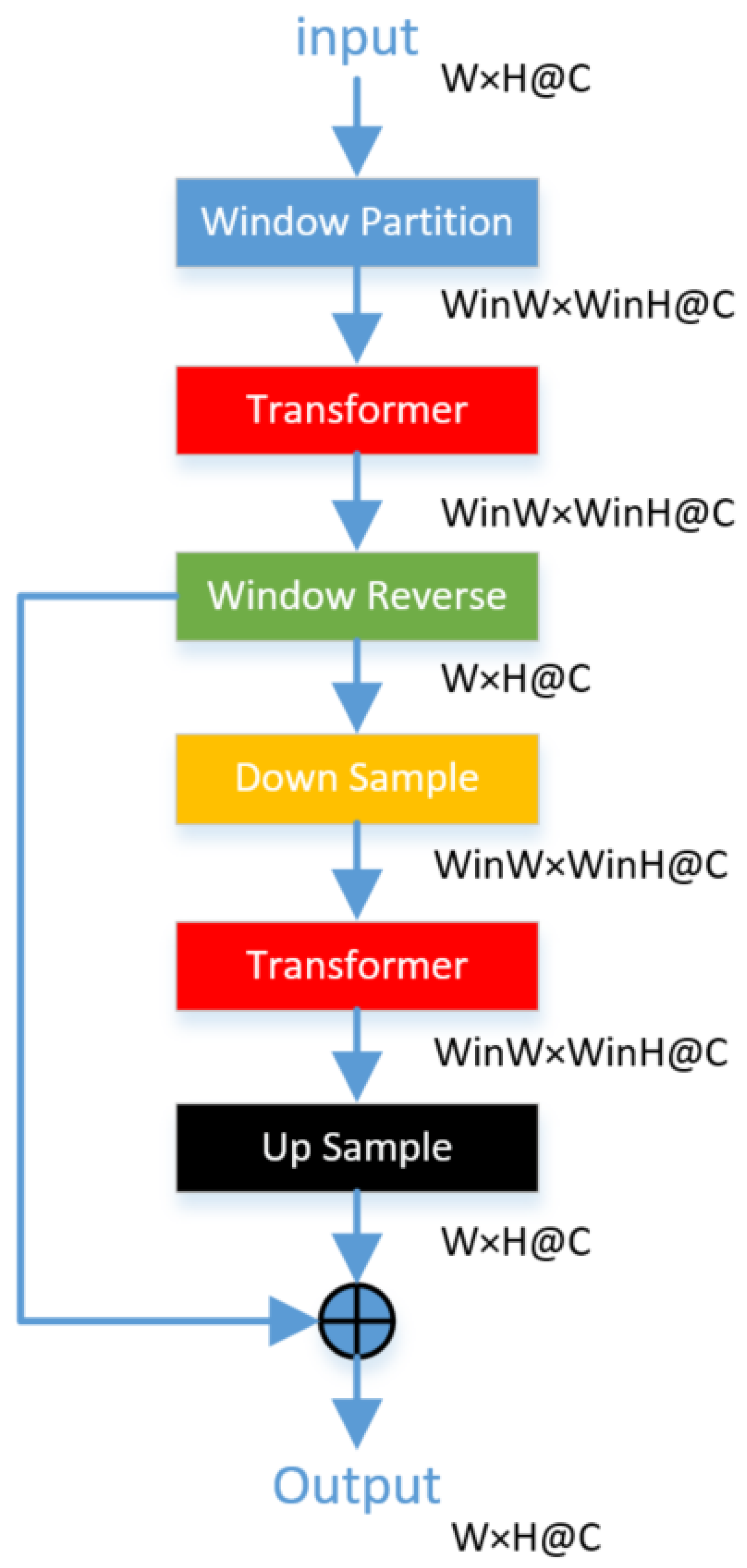
To address the limitation of Swin Transformer’s window-shifting method indirectly expanding the receptive field to cover the entire image, we propose a module called Nswin Transformer (Non shift window Transformer), as depicted in Figure 3.

In Figure 3, the input feature map has a size of H×W@C. Then, the feature map is partitioned into several patches according to the window size, with each patch’s size being the window’s H×window’s W@C. Each patch undergoes computation using the same transformer; then, these patches are stitched back to the original feature map size, resulting feature map B with a size of H×W@C. To facilitate pixel interaction between windows, feature map B is downsampled to the window size, resulting in feature map C with a size of the window’s H×window’s W@C. Feature map C undergoes Transformer operations, yielding feature map D with a global receptive field. To fuse the global features from D into each pixel, feature map D is upsampled to the size of the input feature map, then added to feature map B, which is computed by the window Transformer, resulting in feature map E with integrated global features. Feature map E retains the same size and channel number as the input feature map, ensuring that the Nswin Transformer module does not alter the feature map’s size or channel number. The pseudocode for the Nswin Trans-former module is shown in Algorithm 1.

Algorithm 1 Nswin Transformer

1:  procedure NswinTransformer   2:     Input: feature map   3:     Output: feature map   4:     The input feature map is partitioned into several patches by window to obtain the feature map A.   5:     All patches undergo computation using the same window Transformer, and then these patches are stitched back to the original feature map size, resulting in feature map B.   6:     Feature map B is downsampled to the window size, resulting in feature map C.   7:     Feature map C undergoes Transformer operations, resulting in feature map D.   8:     Feature map D is upsampled to the size of the input feature map and then added to feature map B, resulting in feature map E.   9:     return feature map E. 10:  end procedure

3.2. Nswin Transformer Net

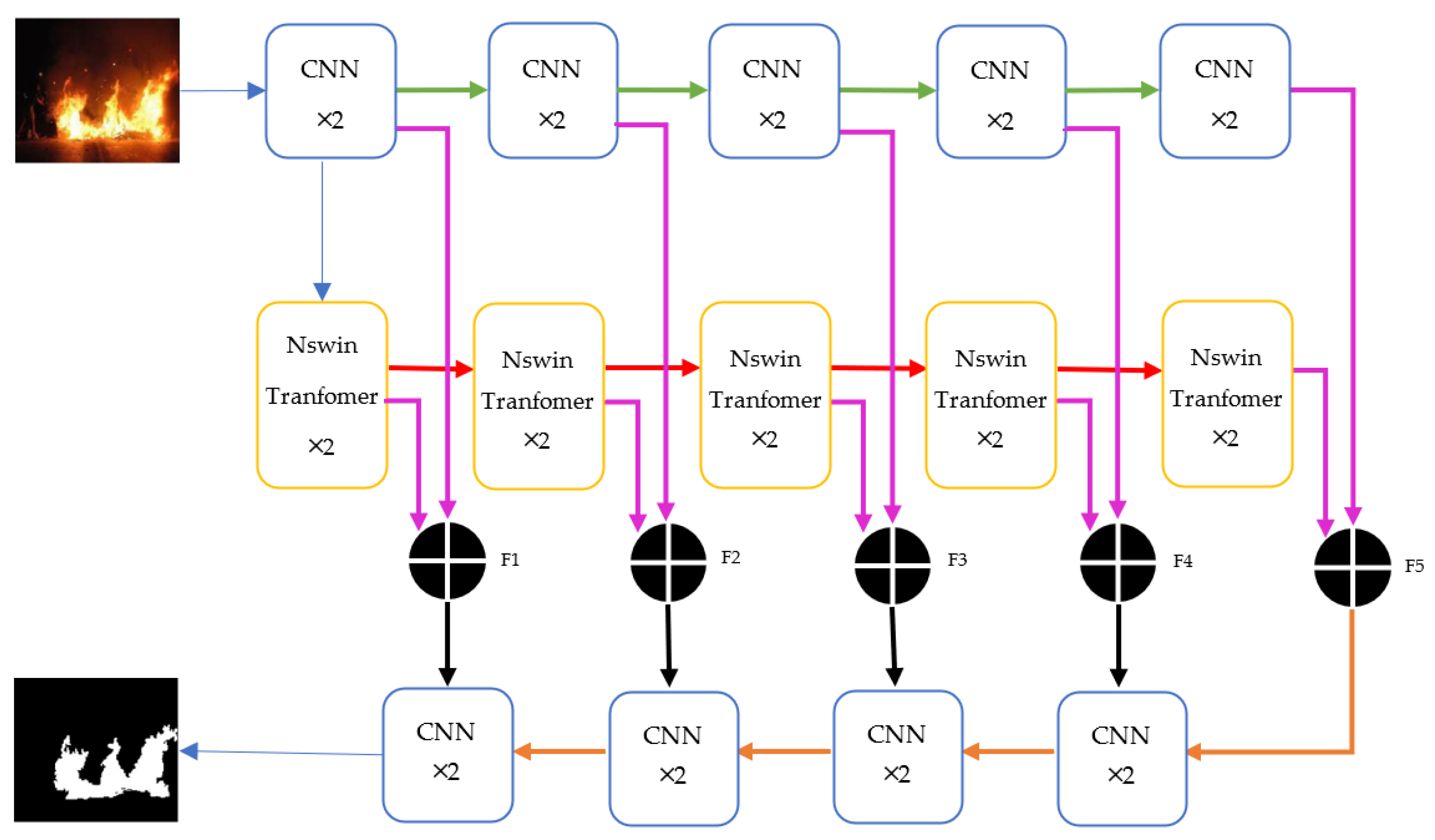
The Nswin Transformer module is adept at capturing global features. However, local features are also crucial, and an overemphasis on global information can obscure significant local details. To address this, we introduce the Nswin Transformer Network, which synergizes the strengths of convolutional neural networks (CNNs) and Nswin Transformer modules. In this network, CNNs are employed to effectively extract local features, while Nswin Transformer modules focus on global feature extraction. These two feature types are then integrated in each layer and gradually upsampled to match the input image size. The architecture of the Nswin Transformer Network is illustrated in Figure 4.

The encoding part of the Nswin Transformer Network abandons the 4-layer structure of Swin Transformer and adopts the same 5-layer structure as UNet. The encoding part consists of the following two components: CNNs for capturing local features and Nswin Transformer blocks for capturing global features.

The CNN consists of 2D convolutions with a kernel size of 3 × 3 and a stride of 1, followed by BatchNorm and ReLU activations. The input image passes through the first layer of 2 CNNs, resulting in a feature map size of 256 × 256@64. Subsequently, after max-pooling with a stride and window size of 2, both the length and width of the feature map are halved. Then, after two more CNN layers, the second layer’s feature map size becomes 128 × 128@128. Next, by continuing with the same max-pooling configuration as before, followed by 2 CNN layers, the third layer’s feature map size becomes 64 × 64@256. The max pooling, stride, window size, and CNN kernel size and stride for the fourth and fifth layers are all the same as those used in the previous layers. Consequently, we obtain a fourth-layer feature map size of 32 × 32@512 and a fifth-layer feature map size of 16 × 16@1024.

To effectively integrate global and local features in each layer, our global feature extraction part uses a 5-layer architecture. Each layer consists of 2 Nswin Transformer modules with a fixed window size of 8, and they all employ multi-head attention mechanisms. The number of attention heads increases progressively from 1 head for the first layer, to 2 heads for the second, 4 for the third, 8 for the fourth, and 16 for the fifth. Since the Nswin Transformer modules cannot alter the number of channels, the input to the global feature extractor is the feature map from the first layer of the CNN, with a size of 256 × 256@64. After processing through two Nswin Transformer modules in the first layer, the feature map retains its size of 256 × 256@64. Following this, a patch-merging module reduces the feature map’s dimensions by half. The output from the second layer, after passing through its two Nswin Transformer modules, results in a feature map of 128 × 128@128. This halving and processing pattern continues for the subsequent layers, producing feature maps of 64 × 64@256, 32 × 32@512, and 16 × 16@1024 for the third, fourth, and fifth layers, respectively.

Before decoding, the local features and global features of five layers are added separately in each layer to obtain feature maps F1, F2, F3, F4, and F5. Then, the same stepwise upsampling method is used as in UNet. The decoding part of the CNN is the same as the encoding part, consisting of 2D convolutions with a kernel size of 3 × 3 and a stride of 1, batch normalization, and ReLU activation. The upsampling module increases both the length and width of the feature maps by a factor of two, using an upsampling module, 2D convolutions with a kernel size of 3 × 3 and a stride of 1, batch normalization, and ReLU activation. After the feature map F5 is upsampled, its size becomes 32 × 32@512; then, it is concatenated with feature map F4, and after passing through two CNN modules, a feature map with a size of 32 × 32@512 is obtained. Subsequently, the same procedure is repeated to concatenate F3, F2, and F1, resulting in a feature map with a size of 256 × 256@64. Finally, after a 2D convolution with a kernel size of 1 and a stride of 1, the output size becomes 256 × 256@2.

3.3. Evaluation Metrics

We use the F1 score, consisting of precision and recall, as an evaluation metric, as well as mIoU (Mean Intersection over Union) and OA (Overall Accuracy). These three metrics are used to evaluate each deep learning model. They are calculated as shown in Equations (2)–(6).

The formula for mIoU is

$$\mathrm{mIoU}={\displaystyle \frac{1}{N+1}}\sum _{i=0}^N{\displaystyle \frac{TP}{TP+FN+FP}},$$

(1)

where N is the number of foreground pixels; TP is the abbreviation of true positives, that is, the number of pixels correctly predicted as the foreground; FP is the abbreviation of false positives, that is, the number of background pixels misjudged as the foreground; TN is the abbreviation of true negatives, that is, the number of pixels correctly predicted as the background; and FN is the abbreviation of false negatives, that is, the number of foreground pixels misjudged as background.

The formula for OA is

$$\mathrm{Accuracy}={\displaystyle \frac{TP+TN}{TP+TN+FP+FN}}.$$

(2)

The formula for the F1 score is.

$$\mathrm{F}1-\mathrm{Score}={\displaystyle \frac{2\times Precison\times Recall}{Precison+Recall}},$$

(3)

where precision and recall are

$$Precision={\displaystyle \frac{TP}{TP+FP}}$$

(4)

$$Recall={\displaystyle \frac{TP}{TP+FN}}.$$

(5)

In Equation (3), fire and background are regarded as the foreground to obtain the IoU; then, the average value is taken as the mIoU. The foreground in Equations (4)–(6) is fire.

3.4. Hardware and Software for Experiments

The hardware and software configurations used in this experiment are shown in the

Table 1. Hardware and software details.

Hardware and Software	Parameters
CPU	Intel Intel i5-13600KF
GPU	NVIDIA GeForce RTX 2080Ti
Operating memory	32 GB
Total video memory	22 GB
Operating system	Ubuntu 22.04.4
Python	Python 3.10.12
IDE	PyCharm 2022.1.4
CUDA	CUDA 12.1
CUDNN	CUDNN 8.9.6
Deep learning architecture	PyTorch 2.0.1

.

The hardware configuration of the computer used for the experiments is summarized as follows: CPU, is Intel i5-13600KF; RAM, SEIWHALE DDR4 16G × 2; and GPU, NVIDIA GeForce RTX 2080TI 22G. The version of Python is 3.10.12, and Pytorch is used as the deep learning framework for model training and evaluation.

AdamOptimizer was used for back propagation, the batch size was set to 4, and the learning rate was set to 0.0001 during training. Because the default EPS is too small, which can cause some models to have a LOSS of NAN during training, we set the EPS to 0.003. The sum of L2 regularization and binary cross entropy was used as the total loss to prevent overfitting. The total loss is shown in Formula (1). The maximum number of training epochs was set to 300. After each epoch, an evaluation was performed on the validation dataset. Unlike the stopping standard used in ShiftPoolingPSPNet [54], in which training was stopped if the metrics in the validation set no longer increased for 10 consecutive epochs, our stopping standard was set such that if the loss in the test dataset no longer reduced for 20 consecutive epochs, then training was stopped.

$$\begin{gathered} \mathrm{TotalLoss}=\mathrm{BinaryCrossEntropy}+L2 \\ L2={\Vert w\Vert }_2^2=\sum _i\mid w_i^2\mid \end{gathered}$$

(6)

The specific experimental steps are listed as follows:

(1) Set parameters;

(2) Read training sample data in batches;

(3) Train on all training data;

(4) Evaluate on the test set;

(5) Repeat steps (3) and (4) until the stopping condition is met;

(6) Segment the test-set images.

4. Experimental Results

4.1. Results on the Corsican Fire Dataset

To objectively demonstrate the superiority of our proposed Nswin Transformer Net, we employed three objective evaluation metrics, namely mIoU (mean intersection over union), F1 score, and OA (overall accuracy). We trained SegNet, UNet, PSPNet, ShiftPoolingPSPNet, NestedUNet, and our Nswin Transformer Net on the dataset and performed validation on the test set. The metric values for each network are shown in

Table 2. Results of classic semantic segmentation on the Corsican Fire test dataset.

Method	mIoU (%)	F1 Score (%)	OA (%)
SegNet	73.5	68.1	95.6
UNet	76.9	73.4	96.2
PSPNet	76.8	72.8	96.5
ShiftPoolingPSPNet	77.1	73.7	96.1
NestedUNet	78.0	74.5	96.7
Nswin Transformer Net	79.4	76.6	96.9

.

From Table 2, it can be observed that SegNet performed the worst among all models, with the lowest mIoU, F1 score, and OA values of 73.5, 68.1, and 95.6, respectively. Its mIoU is 3.4 lower than that of UNet, the F1 score is 5.3 lower, and its OA is 0.6 lower. Despite being an improvement over UNet, according to our experiments on the dataset used in this study, SegNet’s performance is inferior to that of UNet. This could be attributed to significant differences between the test set and the training set, indicating poor generalization of SegNet. We used ResNet50 as the backbone for PSPNet in our experiments. PSPNet performed comparably to UNet, with mIoU and F1-score values slightly lower by 0.1 and 0.6, respectively, although the OA was higher by 0.3. ShiftPooling performed slightly better than UNet and PSPNet, with mIoU, F1-score, and OA values of 77.1, 73.7, and 96.1, respectively. NestedUNet showed significant improvement over the previous models, with mIoU, F1-score, and OA values of 78.0, 74.5, and 96.7, respectively, indicating better generalization of NestedUNet compared to the previous models. The best performance was achieved by our proposed Nswin Transformer Net, which combines local features and improves upon the Swin Transformer architecture. Nswin Transformer net achieved mIoU, F1-score, and OA values of 79.4, 76.6, and 96.9, respectively, indicating that our proposed Nswin Transformer net can effectively capture image features more efficiently and has better generalization capabilities than the compared models.

Figure 5 displays the prediction results of each model on a fire image from the test set. The first image on the left in the top row is the input fire image, the second image is the ground truth, the third image is the prediction from SegNet, and the fourth image is the prediction from PSPNet. The second row, from left to right, shows the predictions from UNet, ShiftPoolingPSPNet, NestedUNet, and Nswin Transformer Net. In the images, red pixels represent false negatives, indicating pixels where fire was missed in the prediction. Green pixels represent false positives, indicating background pixels that were incorrectly classified as fire. Black pixels represent true negatives, and white pixels represent true positives.

From the various prediction images, it can be observed that SegNet has a considerable number of both red and green pixels, indicating a high rate of both false negatives and false positives. This aligns with the lower metric values shown in Table 2. PSPNet, despite having fewer green pixels, has a significant number of red pixels, indicating a low false-positive rate but a high false-negative rate. On the other hand, UNet shows the opposite pattern compared to PSPNet; it has almost no red pixels but more green pixels, indicating a higher false positive rate and a lower false-negative rate. ShiftPoolingPSPNet and NestedUNet exhibit similar characteristics, with both having fewer red and green pixels compared to UNet and PSPNet. Additionally, the quantities of red and green pixels are relatively balanced. This suggests that ShiftPoolingPSPNet and NestedUNet perform slightly better overall compared to the previous models. The best performance is achieved by our proposed Nswin Transformer Net. Leveraging better global feature capturing and local feature fusion capabilities, Nswin Transformer Net has significantly fewer red and green pixels, indicating lower false-positive and false-negative rates. This demonstrates a closer alignment with the ground truth.

4.2. Results on the FLAME Dataset

To further validate our model, we conducted the same experiments on both the FLAME and BoWFire Datasets. The metric values for each network are shown in

Table 3. Results of classic semantic segmentation on the FLAME test dataset.

Method	mIoU (%)	F1 Score (%)	OA (%)
SegNet	81.8	77.9	99.8
UNet	83.7	80.6	99.8
PSPNet	80.2	75.5	99.8
ShiftPoolingPSPNet	82.0	78.2	99.8
NestedUNet	83.9	80.9	99.9
Nswin Transformer Net	84.4	81.6	99.9

.

From Table 3, it can be observed that the PSPNet model performs the worst, with mIoU, F1-score, and OA values of only 80.2, 75.5, and 99.8, respectively. On the other hand, the ShiftPoolingPSPNet model, which employs the shift pooling method to increase the receptive field of edge pixels in the pooling grid, shows improved accuracy, with mIoU, F1-score, and OA values of 82.0, 78.2, and 99.8, respectively. However, both of these models perform relatively poorly compared to others, which is inconsistent with Table 2. This suggests that PSPNet performs worse in small object segmentation than in large object segmentation. SegNet performs slightly worse than ShiftPoolingPSPNet, while the structurally similar UNet shows a significant improvement in accuracy, achieving mIoU, F1-score, and OA values of 83.7, 80.6, and 99.8, respectively. This is consistent with its performance on the Corsican Fire dataset, indicating that SegNet, with its index-based upsampling, performs worse than interpolation-based upsampling on these two datasets. NestedUNet shows slightly better performance than UNet, with mIoU, F1-score, and OA values reaching 83.9, 80.9, and 99.9, respectively. Our model performs the best, with mIoU and F1-score values 0.5 and 0.7 higher than the second-best model NestedUNet, respectively. Since the FLAME dataset has a relatively uniform data format, the differences in metrics between various models are not substantial. Therefore, a 0.5 improvement is considered quite significant.

It is worth mentioning that the OA values for all models are almost identical. This is because the proportion of fire pixels in the dataset is very small, so if the model makes errors in predicting fire pixels, it has a relatively small impact on the OA value. Therefore, mIoU and F1 score are more indicative of the model’s performance.

Figure 6 displays the prediction results of each model on a fire image from the FLAME test dataset. The first image on the left in the top row is the input fire image, the second image is the ground truth, the third image is the prediction from SegNet, and the fourth image is the prediction from UNet. The second row, from left to right, shows the predictions from PSPNet, ShiftPoolingPSPNet, NestedUNet, and Nswin Transformer Net. In the image, red pixels represent false negatives, indicating pixels where fire was missed in the prediction. Green pixels represent false positives, indicating background pixels that were incorrectly classified as fire. Black pixels represent true negatives, and white pixels represent true positives.

From Figure 6, it can be observed that the proportion of fire pixels in the entire image is very small, indicating a problem in small object segmentation. However, all models’ prediction maps contain fire, with very few false-positive (green) and false-negative (red) pixels. The absence of red pixels is particularly notable, meaning that the proportion of incorrectly predicted pixels in all models’ prediction maps is very small, consistent with the OA values of all models in Table 3. Additionally, all models accurately predict the background, with very few false-positive pixels around the fire, indicating that no pixels outside the fire region are mistakenly classified as fire. This is because the background pixels make up a large proportion of the image, allowing the models to effectively extract background features during training. In the prediction maps of Nswin Transformer and NestedUNet, there are visibly fewer green pixels compared to SegNet, UNet, PSPNet, and ShiftPoolingPSPNet. However, NestedUNet has a small amount of red pixels, whereas Nswin Transformer has none. This suggests that employing the Nswin Transformer architecture allows each layer’s window Transformer to have a global receptive field, thereby enhancing the accuracy of small object segmentation.

4.3. Ablation Experiment

In order to investigate the contribution of each module in Nswin Transformer Net and whether Nswin Transformer is more effective than Swin Transformer, we conducted ablation experiments, the results of which are shown in

Table 4. Ablation experiment on test datase.

Method	mIoU (%)	F1 Score (%)	OA (%)
SwinTransformer	76.7	73.1	96.0
Swin Transformer + CNN	78.1	74.8	96.6
Nswin Transformer + CNN	79.4	76.6	96.9

. It can be observed that when using only the Swin Transformer module to capture global features, the mIoU was only 76.7, the F1 score was 73.1, and the accuracy was 96.0. After adding the CNN module to capture local features, mIoU, F1 score, and OA increased to 78.1, 74.8, and 96.6, respectively. Subsequently, replacing Swin Transformer with Nswin Transformer led to further improvements in all three metrics, reaching 79.4, 76.6, and 96.9, respectively. This demonstrates that our proposed Nswin Transformer module outperforms Swin Transformer, and the incorporation of a CNN also effectively enhances metric values.

To verify whether our method results in a significant decrease in computational speed compared to Swin Transformer, we conducted a comparative analysis of the FLOPs (Floating Point Operations) for each module. The results are shown in

Table 5. Comparison of different module parameter values.

Method	FLOPs (GMac)
SwinTransformer	83.32
Swin Transformer + CNN	97.87
Nswin Transformer + CNN	100.02

.

From Table 5, we can observe the following: when using an encoder with only Swin Transformer modules (distinct from the original Swin Transformer, our implementation employs a five-scale encoding similar to UNet, where each scale includes a Window Transformer and a Shift Window Transformer), the FLOPs (floating point operations) are 83.32 GMac. When we incorporate CNN modules, the encoding stage at each of the five scales integrates both local and global features, and the FLOPs increase to 97.87 GMac. In our proposed method, while retaining the same CNN modules, we replace the Swin Transformer modules at all five scales with Nswin Transformer modules, and we see that the FLOPs only increase by 2.15 GMac.

5. Discussion

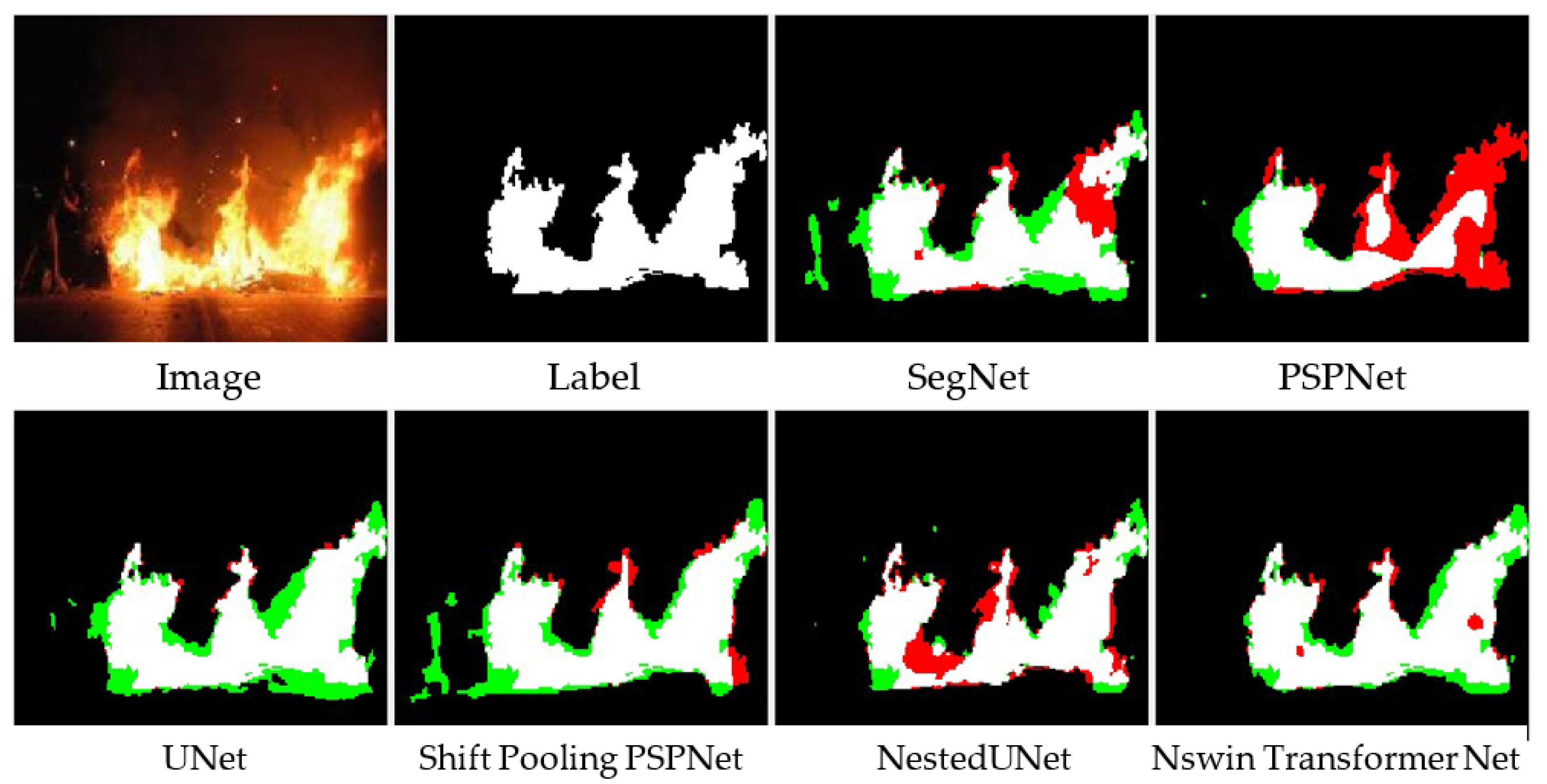
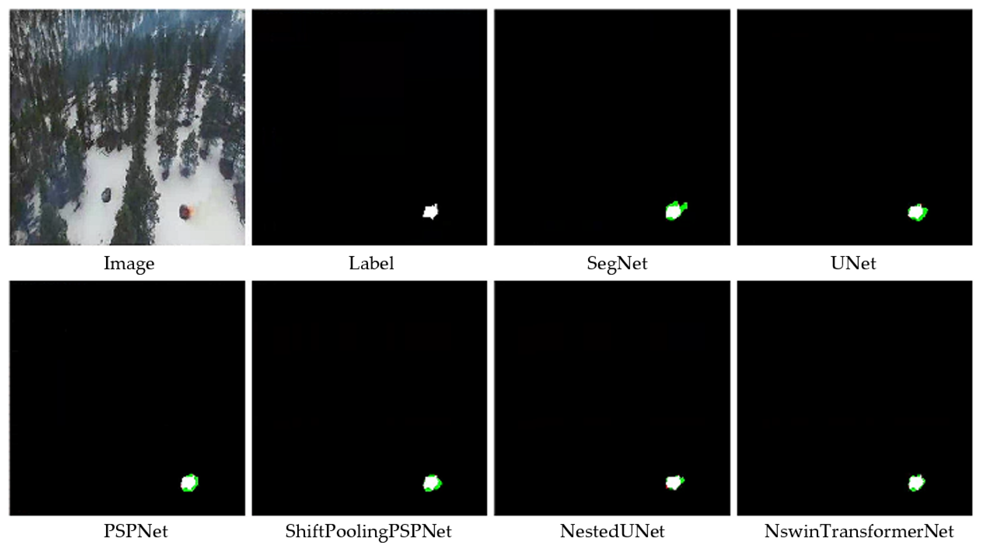
By introducing a transformer, Nswin Transformer Nets can capture global features in each layer after the window transformer. This significantly enhances the network’s feature-capturing ability. Experimental results on two datasets demonstrate that our proposed method performs the best in terms of mIoU, F1 score, and OA. Notably, on the Corsican Fire Dataset, our Nswin Transformer Net surpasses the second-best NestedUNet by 1.4% in mIoU, 2.1% in F1 score, and 0.2% in OA. This is a significant improvement, considering that the second-best NestedUNet only surpasses the third-best ShiftPoolingPSPNet by 0.6%, 1.1%, and 0.6% in mIoU, F1 score, and OA, respectively. Given that the proportion of fire pixels in the FLAME dataset is very small, achieving improvements in mIoU, F1 score, and OA is particularly challenging. However, our Nswin Transformer Net still outperforms the second-best NestedUNet by 0.5% in mIoU and 0.7% in F1 score.

From the ablation experiments, it can be observed that under the same network architecture and convolutional modules, our proposed Nswin Transformer module performs better than the original Swin Transformer module, with improvements of 1.3%, 1.8%, and 0.3% in mIoU, F1 score, and OA, respectively. This highlights the importance of enhancing global feature capture at each scale. Although this leads to a slight increase of 2.15 GMac in FLOPs, it is negligible compared to the 14.55 GMac increase caused by using only CNNs.

6. Conclusions

In this paper, we propose a network called Nswin Transformer Net aimed at addressing the limitations of Swin Transformer, which requires multiple layers to capture global features. Through detailed experimental validation and comparative analysis, we demonstrate that this network achieves significant performance improvements across multiple datasets.

Specifically, on the Corsican Fire Dataset, our Nswin Transformer Net achieved mIoU, F1-score, and OA values of 79.4, 76.6, and 96.9, respectively, surpassing the second-best NestedUNet by 1.4% in mIoU, 2.1% in F1 score, and 0.2% in OA. On the FLAME dataset, Nswin Transformer Net still outperforms the second-best NestedUNet by 0.5% in mIoU and 0.7% in F1 score. These results indicate that our the design of our Nswin Transformer model eliminates the limitation of Swin Transformer requiring multiple layers to capture global features, enabling the network to capture global features in each layer, thereby enhancing the global feature-capturing ability of the shallow network. This significantly improves the accuracy of fire image segmentation.

Furthermore, we conducted an in-depth analysis of the impact of each module in the Nswin Transformer network on accuracy and computational load. With other conditions unchanged, replacing Swin Transformer with Nswin Transformer improves mIoU, F1 score, and OA by 1.3%, 1.8%, and 0.3%, respectively, while increasing the computational load by only 2.15 GMac. Therefore, Nswin Transformer can significantly improve fire image segmentation accuracy with a minimal increase in computational load.

In conclusion, our proposed Nswin Transformer Net further improves upon the Swin Transformer. In our future work, we will further explore methods to maintain the capability of capturing global features in each layer of the window transformer while reducing computational complexity to improve processing speed.

References

1. Peñuelas, J.; Sardans, J. Global Change and Forest Disturbances in the Mediterranean Basin: Breakthroughs, Knowledge Gaps, and Recommendations. Forests 2021, 12, 603. [Google Scholar] [CrossRef]
2. Davide, A.; Jose, V.; Marco, M.; Lorenzo, S. Land use change towards forests and wooded land correlates with large and frequent wildfires in Italy. Ann. Silvic. Res. 2021, 46, 177–188. [Google Scholar]
3. Sadowska, B.; Grzegorz, Z.; Stępnicka, N. Forest Fires and Losses Caused by Fires–An Economic Approach. WSEAS Trans. Environ. Dev. 2021, 17, 181–191. [Google Scholar] [CrossRef]
4. Zhang, J.; Li, W.; Yin, Z.; Liu, S.; Guo, X. Forest fire detection system based on wireless sensor network. In Proceedings of the 2009 4th IEEE Conference on Industrial Electronics and Applications, Xi’an, China, 25–27 May 2009. [Google Scholar] [CrossRef]
5. Yu, L.; Wang, N.; Meng, X. Real-time forest fire detection with wireless sensor networks. In Proceedings of the 2005 International Conference on Wireless Communications, Networking and Mobile Computing, Wuhan, China, 26 September 2005. [Google Scholar] [CrossRef]
6. Chen, S.J.; Hovde, D.C.; Peterson, K.A.; Marshall, A.W. Fire detection using smoke and gas sensors. Fire Saf. J. 2007, 42, 507–515. [Google Scholar] [CrossRef]
7. Horng, W.B.; Peng, J.W.; Chen, C.Y. A new image-based real-time flame detection method using color analysis. In Proceedings of the 2005 IEEE Networking, Sensing and Control, Tucson, AZ, USA, 19–22 March 2005. [Google Scholar] [CrossRef]
8. Çelik, T.; Demirel, H. Fire detection in video sequences using a generic color model. Fire Saf. J. 2009, 44, 147–158. [Google Scholar] [CrossRef]
9. Chen, T.; Wu, P.; Chiou, Y. An early fire-detection method based on image processing. In Proceedings of the 2004 International Conference on Image Processing, Singapore, 24–27 October 2004. [Google Scholar]
10. Collumeau, J.F.; Laurent, H.; Hafiane, A.; Chetehouna, K. Fire scene segmentations for forest fire characterization: A comparative study. In Proceedings of the 2011 18th IEEE International Conference on Image Processing, Brussels, Belgium, 11–14 September 2011. [Google Scholar] [CrossRef]
11. Ferreira, L.M.; Coimbra, A.P.; de Almeida, A.T. Autonomous System for Wildfire and Forest Fire Early Detection and Control. Inventions 2020, 5, 41. [Google Scholar] [CrossRef]
12. Resco de Dios, V.; Nolan, R.H. Some Challenges for Forest Fire Risk Predictions in the 21st Century. Forests 2021, 12, 469. [Google Scholar] [CrossRef]
13. Qiu, T.; Yan, Y.; Lu, G. An Autoadaptive Edge-Detection Algorithm for Flame and Fire Image Processing. IEEE Trans. Instrum. Meas. 2012, 61, 1486–1493. [Google Scholar] [CrossRef]
14. Chino, D.Y.T.; Avalhais, L.P.S.; Rodrigues, J.F.; Traina, A.J.M. BoWFire: Detection of Fire in Still Images by Integrating Pixel Color and Texture Analysis. In Proceedings of the 2015 28th SIBGRAPI Conference on Graphics, Patterns and Images, Salvador, Brazil, 26–29 August 2015. [Google Scholar] [CrossRef]
15. Chen, J.; He, Y.; Wang, J. Multi-feature fusion based fast video flame detection. Build. Environ. 2010, 45, 1113–1122. [Google Scholar] [CrossRef]
16. Jamali, M.; Karimi, N.; Samavi, S. Saliency Based Fire Detection Using Texture and Color Features. In Proceedings of the 2020 28th Iranian Conference on Electrical Engineering (ICEE), Tabriz, Iran, 4–6 August 2020. [Google Scholar] [CrossRef]
17. Celik, T.; Demirel, H.; Ozkaramanli, H.; Uyguroglu, M. Fire detection using statistical color model in video sequences. J. Vis. Commun. Image Represent. 2007, 18, 176–185. [Google Scholar] [CrossRef]
18. Ko, B.C.; Ham, S.J.; Nam, J.Y. Modeling and Formalization of Fuzzy Finite Automata for Detection of Irregular Fire Flames. IEEE Trans. Circuits Syst. Video Technol. 2011, 21, 1903–1912. [Google Scholar] [CrossRef]
19. LeCun, Y.; Bengio, Y.; Hinton, G. Deep learning. Nature 2015, 521, 436–444. [Google Scholar] [CrossRef]
20. Guan, Z.; Miao, X.; Mu, Y.; Sun, Q.; Ye, Q.; Gao, D. Forest Fire Segmentation from Aerial Imagery Data Using an Improved Instance Segmentation Model. Remote Sens. 2022, 13, 3159. [Google Scholar] [CrossRef]
21. Vasconcelos Reinolds de Sousa, J.; Vieira Gamboa, P. Aerial Forest Fire Detection and Monitoring Using a Small UAV. KnE Eng. 2020, 5, 242–256. [Google Scholar] [CrossRef]
22. Sudhakar, S.; Vijayakumar, V.; Kumar, C.; Priya, V.; Ravi, L.; Subramaniyaswamy, V. Unmanned Aerial Vehicle (UAV) based Forest Fire Detection and monitoring for reducing false alarms in forest-fires. Comput. Commun. 2020, 149, 1–16. [Google Scholar] [CrossRef]
23. Chen, Y.; Zhang, Y.; Xin, J.; Yi, Y.; Liu, D.; Liu, H. A UAV-based forest fire-detection algorithm using convolutional neural network. In Proceedings of the 2018 37th Chinese Control Conference (CCC), Wuhan, China, 25–27 July 2018; pp. 10305–10310. [Google Scholar]
24. Zhang, L.; Wang, M.; Fu, Y.; Ding, Y. A Forest Fire Recognition Method Using UAV Images Based on Transfer Learning. Forests 2022, 13, 975. [Google Scholar] [CrossRef]
25. Kuutti, S.; Bowden, R.; Jin, Y.; Barber, P.; Fallah, S. A survey of deep learning applications to autonomous vehicle control. IEEE Trans. Intell. Transp. Syst. 2020, 22, 712–733. [Google Scholar] [CrossRef]
26. Tian, Y.; Luo, P.; Wang, X.; Tang, X. Deep learning strong parts for pedestrian detection. In Proceedings of the IEEE International Conference on Computer Vision, Santiago, Chile, 7–13 December 2015; pp. 1904–1912. [Google Scholar]
27. Pérez-Hernández, F.; Tabik, S.; Lamas, A.; Olmos, R.; Fujita, H.; Herrera, F. Object detection binary classifiers methodology based on deep learning to identify small objects handled similarly: Application in video surveillance. Knowl.-Based Syst. 2020, 194, 105590. [Google Scholar] [CrossRef]
28. Nawaratne, R.; Alahakoon, D.; De Silva, D.; Yu, X. Spatiotemporal anomaly detection using deep learning for real-time video surveillance. IEEE Trans. Ind. Inform. 2019, 16, 393–402. [Google Scholar] [CrossRef]
29. Lecun, Y.; Bottou, L.; Bengio, Y.; Haffner, P. Gradient-based learning applied to document recognition. Proc. IEEE 1998, 86, 2278–2324. [Google Scholar] [CrossRef]
30. Gonzalez, A.; Zuniga, M.; Nikulin, C.; Carvajal, G.; Cardenas, D.; Pedraza, M.; Fernandez, C.; Munoz, R.; Castro, N.; Rosales, B.; et al. Accurate Fire Detection through Fully Convolutional Network. In Proceedings of the 7th Latin American Conference on Networked and Electronic Media (LACNEM 2017), Valparaiso, Chile, 6–7 November 2017. [Google Scholar] [CrossRef]
31. Krizhevsky, A.; Sutskever, I.; Hinton, G.E. ImageNet Classification with Deep Convolutional Neural Networks. Commun. ACM 2017, 60, 84–90. [Google Scholar] [CrossRef]
32. Muhammad, K.; Ahmad, J.; Lv, Z.; Bellavista, P.; Yang, P.; Baik, S.W. Efficient Deep CNN-Based Fire Detection and Localization in Video Surveillance Applications. IEEE Trans. Syst. Man Cybern. Syst. 2019, 49, 1419–1434. [Google Scholar] [CrossRef]
33. Iandola, F.; Han, S.; Moskewicz, M.; Ashraf, K.; Dally, W.; Keutzer, K. SqueezeNet: AlexNet-level accuracy with 50x fewer parameters and <0.5MB model size. arXiv 2016, arXiv:1602.07360. [Google Scholar]
34. Vaswani, A.; Shazeer, N.; Parmar, N.; Uszkoreit, J.; Jones, L.; Gomez, A.N.; Kaiser, Ł.; Polosukhin, I. Attention is all you need. In Proceedings of the Neural Information Processing Systems (NeurIPS), Long Beach, CA, USA, 4–9 December 2017. [Google Scholar]
35. Liu, Z.; Lin, Y.; Cao, Y.; Hu, H.; Wei, Y.; Zhang, Z.; Lin, S.; Guo, B. Swin transformer: Hierarchical vision transformer using shifted windows. In Proceedings of the 2021 IEEE/CVF International Conference on Computer Vision (ICCV), Montreal, QC, Canada, 10–17 October 2021. [Google Scholar] [CrossRef]
36. Jadon, A.; Omama, M.; Varshney, A.; Ansari, M.; Sharma, R. Firenet: A specialized lightweight fire smoke detection model for real-time iot applications. arXiv 2019, arXiv:1909.07981. [Google Scholar]
37. Raspberry pi 3 Model b. Available online: https://www.raspberrypi.org/products/raspberry-pi-3-model-b/ (accessed on 14 March 2019).
38. Wang, G.; Wang, F.; Zhou, H.; Lin, H. Fire in focus: Advancing wildfire image segmentation by focusing on fire edges. Forests 2024, 15, 217. [Google Scholar] [CrossRef]
39. Zhao, H.; Shi, J.; Qi, X.; Wang, X.; Jia, J. Pyramid scene parsing network. In Proceedings of the 2017 IEEE Conference on Computer Vision and Pattern Recognition (CVPR), Honolulu, HI, USA, 21–26 July 2017. [Google Scholar] [CrossRef]
40. Badrinarayanan, V.; Kendall, A.; Cipolla, R. Segnet: A deep convolutional encoder-decoder architecture for image segmentation. In Proceedings of the IEEE Conference on Computer Vision and Pattern Recognition (CVPR), Honolulu, HI, USA, 21–26 July 2017. [Google Scholar]
41. Chen, L.C.; Papandreou, G.; Schroff, F.; Adam, H. Rethinking atrous convolution for semantic image segmentation. arXiv 2017, arXiv:1706.05587. [Google Scholar]
42. Shelhamer, E.; Long, J.; Darrell, T. Fully Convolutional Networks for Semantic Segmentation. IEEE Trans. Pattern Anal. Mach. Intell. 2017, 39, 640–651. [Google Scholar] [CrossRef] [PubMed]
43. Bochkov, V.S.; Kataeva, L.Y. wUUNet: Advanced Fully Convolutional Neural Network for Multiclass Fire Segmentation. Symmetry 2021, 13, 98. [Google Scholar] [CrossRef]
44. Xue, Z.; Lin, H.; Wang, F. A Small Target Forest Fire Detection Model Based on YOLOv5 Improvement. Forests 2022, 13, 1332. [Google Scholar] [CrossRef]
45. Zhu, J.; Zhang, J.; Wang, Y.; Ge, Y.; Zhang, Z.; Zhang, S. Fire Detection in Ship Engine Rooms Based on Deep Learning. Sensors 2023, 23, 6552. [Google Scholar] [CrossRef]
46. Wang, C.Y.; Bochkovskiy, A.; Liao, H.Y. YOLOv7: Trainable bag-of-freebies sets new state-of-the-art for real-time object detectors. In Proceedings of the 2022 IEEE Conference on Computer Vision and Pattern Recognition (CVPR), New Orleans, LA, USA, 18–24 June 2022. [Google Scholar]
47. Ann, H.; Koo, K.Y. Deep Learning Based Fire Risk Detection on Construction Sites. Sensors 2023, 23, 9095. [Google Scholar] [CrossRef] [PubMed]
48. Ultralytics. Ultralytics-Yolov5. Available online: https://github.com/ultralytics/yolov5 (accessed on 5 June 2022).
49. Avazov, K.; Mukhiddinov, M.; Makhmudov, F.; Cho, Y.I. Fire Detection Method in Smart City Environments Using a Deep-Learning-Based Approach. Electronics 2022, 11, 73. [Google Scholar] [CrossRef]
50. Bochkovskiy, A.; Wang, C.Y.; Liao, H.Y. YOLOv4: Optimal Speed and Accuracy of Object Detection. arXiv 2020, arXiv:2004.10934. [Google Scholar]
51. Kim, S.Y.; Muminov, A. Forest Fire Smoke Detection Based on Deep Learning Approaches and Unmanned Aerial Vehicle Images. Sensors 2023, 23, 5702. [Google Scholar] [CrossRef] [PubMed]
52. Toulouse, T.; Rossi, L.; Campana, A.; Celik, T.; Akhloufi, M. Computer vision for wildfire research: An evolving image dataset for processing and analysis. Fire Saf. J. 2017, 92, 188–194. [Google Scholar] [CrossRef]
53. Shamsoshoara, A.; Afghah, F.; Razi, A.; Zheng, L.; Fulé, P.Z.; Blasch, E. Aerial imagery pile burn detection using deep learning: The FLAME dataset. Comput. Netw. 2021, 193, 108001. [Google Scholar] [CrossRef]
54. Yuan, W.; Wang, J.; Xu, W. Shift Pooling PSPNet: Rethinking PSPNet for Building Extraction in Remote Sensing Images from Entire Local Feature Pooling. Remote Sens. 2022, 14, 4889. [Google Scholar] [CrossRef]
Figure 1. Comparison of Swin Transformer and ViT(Vision Transformer). Swin Transformer started with 4× downsampling, followed by 8× downsampling and 16× downsampling. ViT started with 16× downsampling. The red lines are the window boundaries, and the gray lines are the boundaries of each patch.
Forests 15 01337 g001
Figure 2. Window shifting. The left side is the window without shifting. On the right is the window after shifting.
Forests 15 01337 g002
Figure 3. Architecture diagram of the Nswin Transformer module. The black text on the right represents the size of the feature map for each step.
Forests 15 01337 g003
Figure 4. The blue rectangles represent convolutional operation modules consisting of 2D convolutions with a kernel size of 3 × 3, followed by BatchNorm and ReLU. The yellow rectangles represent Nswin Transformer modules. The green arrows represent Maxpooling2D with a kernel size of 2 and a stride of 2. The red arrows represent patch merging. The orange arrows represent ConvTranspose2D with a kernel size of 2 and stride of 2. The purple arrows represent addition. The black arrows represent concatenation.
Forests 15 01337 g004
Figure 5. The output results of each model on the test set. Black represents TN pixels, white represents TP pixels, red represents FN pixels, and green represents FP pixels.
Forests 15 01337 g005
Figure 6. The output results of each model on the FLAME test dataset. Black represents TN pixels, white represents TP pixels, red represents FN pixels, and green represents FP pixels.
Forests 15 01337 g006