An Improved LandTrendr Algorithm for Forest Disturbance Detection Using Optimized Temporal Trajectories of the Spectrum: A Case Study in Yunnan Province, China

Abstract

Forest disturbance mapping plays an important role in furthering our understanding of forest dynamics. The Landsat-based detection of Trends in Disturbance and Recovery (LandTrendr) algorithm is widely used in forest disturbance mapping. However, it neglects the quality of the temporal trajectory and its change trends for forest disturbance mapping. Therefore, the aim of this paper is to improve LandTrendr (iLandTrendr) for forest disturbance mapping by optimizing its temporal trajectories and the post-processing of detection results. Specifically, the temporal trajectory of complex forest disturbance types was optimized using the Savitzky–Golay (SG) filter with constraints. That is, the smooth value generated from the SG filter for the disturbance year was replaced by the satellite observations when the nonlinear abrupt signals were included in the multi-temporal data. The forest disturbance detected by LandTrendr was further modified using the consistency of spectral variation trends. A case study using iLandTrendr to detect forest disturbance in Yunnan Province was conducted. Compared to the LandTrendr method, which has an overall accuracy (OA) of 35.88%, iLandTrendr generated forest disturbance mapping with an OA of 89.32%, which was significantly higher. The total mapped area of disturbance was 1,985,820.9 km², accounting for 49.69% of the total area. The disturbances were predominately caused by natural factors, such as wildfires, pests and diseases, and forest degradation, accounting for 85.31% of the total disturbed area. iLandTrendr can quickly and accurately detect the occurrence year of complex forest disturbance types and can be extended for the forest disturbance mapping of a large area.

1. Introduction

Forest disturbance refers to the phenomenon of a significant decline in or disappearance of forest canopy cover and aboveground biomass caused by natural (e.g., droughts [1], wildfires [2], and pests and diseases [3] caused by climate change) and human-induced factors (e.g., deforestation [4], urbanization [5], and other human-caused problems [6,7]). Forest vegetation absorbs carbon dioxide from the air through photosynthesis and stores a portion of the carbon in forest biomass, deadwood, and soil [8,9]. Forest disturbance events, such as forest fires, logging, or pests and diseases, release carbon stored in living organisms back into the atmosphere [10,11]. Therefore, forest disturbance affects the carbon budget at the regional or global scale [12]. The accurate, timely, and continuous monitoring of forest disturbance, thus, plays a crucial role in sustainable forest management and forest carbon budget measurement at the regional and global scales [13]. Satellite remote sensing data, especially Landsat time-series data, have become an effective means of detecting historical forest disturbance events over a large area due to their advantages of wide coverage, low acquisition costs, and the longest data record (from 1972 to the present). Therefore, seeking to accurately map forest disturbance using the Landsat time-series data has become a popular research topic in forestry remote sensing.

Remote sensing image change detection is widely regarded as an effective method for forest disturbance detection [14]. In recent decades, many algorithms have been proposed for forest disturbance mapping based on Landsat time-series data [15,16,17]. These can be divided into two categories. The first category is change detection using bitemporal remote sensing images [18]. It hypothesizes that forest disturbance occurrence may differ significantly in the spectral reflectance [19] or land cover type [20,21]. The regions with significant differences in two-phase images can be considered forest disturbance. This type of method is simple and efficient, but it is easily affected by plant phenology, and it requires high consistency in the data acquisition time [22], preventing the continuous monitoring of forest disturbances over large areas.

The second category of the method is temporal trajectory change detection [23,24], with the assumption that the temporal trajectory of the spectral index collected from multi-temporal Landsat data without forest disturbance is rising and tends to be stable [25]. The date of forest disturbance can be identified by analyzing and comparing the characteristics of the temporal trajectory at each pixel. This method can be further divided into two subcategories: day scale and year scale. Day-scale methods detect the specific date of forest disturbance using all the available Landsat images, such as CCDC [26], CLOD [27], and CMFDA [28]. Although these algorithms can detect the specific date of forest disturbance, they require a large amount of data storage and computing resources [29]. The year-scale methods detect the year of forest disturbance occurrence using yearly composited Landsat images. For example, Kennedy et al. [30] captured the temporal trajectory of spectral values at each pixel using yearly composited Landsat images from 1984 to 2004, and the year of forest disturbance was identified by comparing the difference between the true and idealized signatures in the entire temporal trajectory. Compared to day-scale methods, this approach requires fewer data storage and computing resources and is more suitable for forest disturbance mapping in large areas [31]. The Landsat-based Detection of Trends in Disturbance and Recovery (LandTrendr) [32] is one of the widely used year-scale algorithms in forest disturbance mapping [33,34,35] due to its computational efficiency and suitability for parallel computing on the Google Earth Engine (GEE) [36,37] cloud platform. Nevertheless, there are still two limitations to LandTrendr that may hinder its applicability for the detection of complex forest disturbance types.

First, LandTrendr adopts a uniform Savitzky–Golay (SG) filter [38] to remove data noise in multi-temporal Landsat data and obtain the smoothed temporal trajectory of all the forest disturbance types, which may introduce uncertainties for certain forest disturbance types. The SG filter is linear, meaning it is difficult to capture the true change trends in abrupt signals, which are nonlinear [28]. The disturbance signals from certain forest disturbance events, especially those with abrupt signals in the multi-temporal data, such as forest fires [2], deforestation [4], and urbanization [5], may be misjudged by the SG filter as data noise [39]. These misjudgments would introduce uncertainties in downstream forest disturbance mapping. However, the precise temporal trajectory of abrupt forest disturbance types can be optimized using the SG filter with constraints. In other words, the smooth value generated from the SG filter for the important years of abrupt forest disturbance events is replaced by satellite observations. This can effectively preserve the real temporal trajectory of complex forest disturbance types. Therefore, it requires modifying the temporal trajectory of complex forest disturbance types to improve LandTrendr for forest disturbance mapping.

Second, LandTrendr relies on a set of control parameters to detect all forest disturbance types, which may reduce the mapping accuracy for certain forest disturbance types [40,41]. The characteristics of the temporal trajectory under different forest disturbance types (e.g., abrupt, gradual, and multiple) can vary significantly [42]. For example, the temporal trajectory of abrupt forest disturbance, such as wildfire, changes rapidly, whereas forest degradation progresses more slowly. Fixed model parameters would result in either the delayed or premature detection of the disturbance year for certain forest disturbance types [42,43,44]. Recently, several methods have been developed to address this limitation. For instance, Li et al. [45] utilized individual disturbance indices and tailored model parameters for regions with different forest types to improve forest disturbance mapping using LandTrendr. In another example, Qiu et al. [46] employed multi-season observations and multi-spectral indices to enhance LandTrendr’s performance in forest disturbance mapping. While these modified algorithms have improved detection accuracy for certain disturbance types, they still rely on fixed model parameters and do not significantly improve the mapping of complex forest disturbances. Additionally, spectral indices such as the normalized burn ratio (NBR) [47], which is highly sensitive to forest disturbance and recovery, are generally lower during the disturbance year than in the preceding or subsequent years. Furthermore, the temporal trajectory generated by satellite observations and the SG filter with constraints should display consistent trends. Therefore, post-processing the detection results based on spectral trend consistency is essential to improve the applicability of LandTrendr for forest disturbance mapping.

In this study, we aimed to improve the LandTrendr (iLandTrendr) from two key perspectives: spectral trajectory optimization and the post-processing of detection results. To achieve this, the three following sub-objectives were set: (1) to optimize the temporal trajectories of complex forest disturbance types; (2) to improve the detected forest disturbance by LandTrendr; and (3) to evaluate the performance of iLandTrendr for forest disturbance mapping at large area.

2. Study Area and Datasets

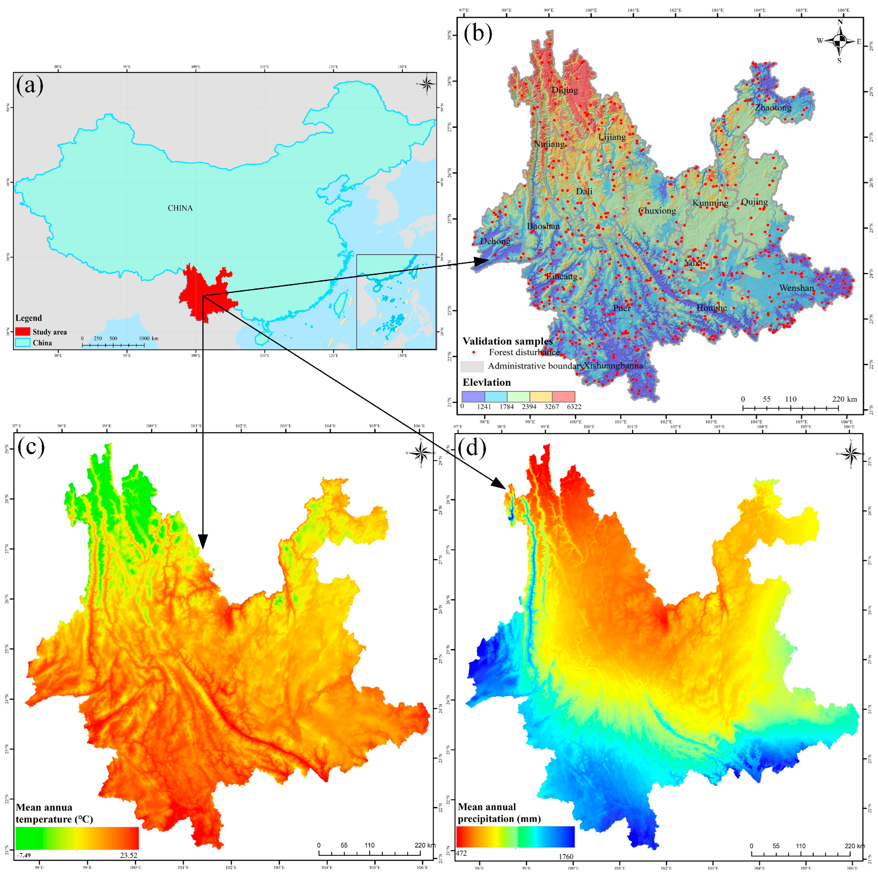
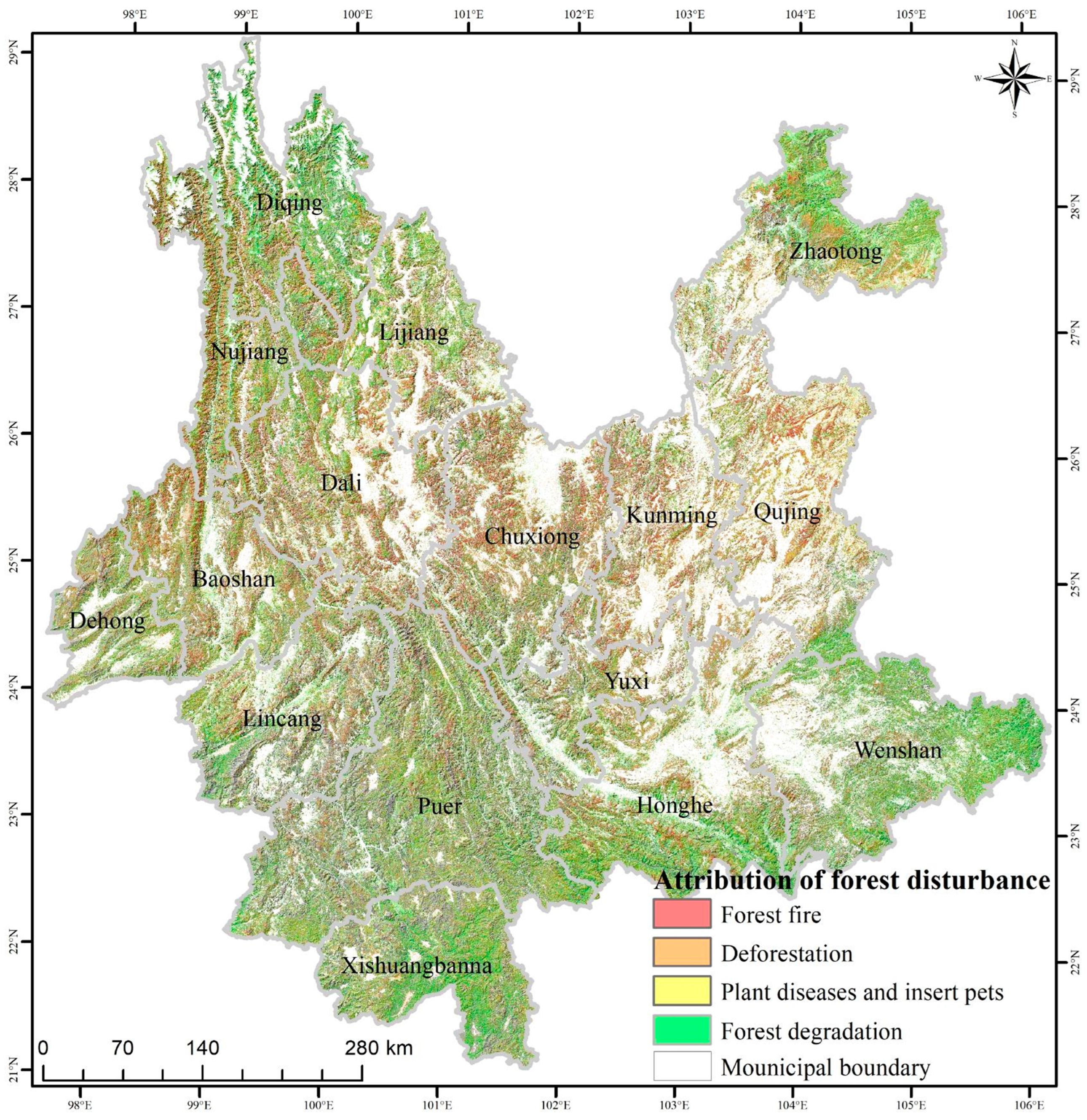
2.1. Study Area

For this study, Yunnan Province (21°8′–29°15′ N, 97°31′–106°11′ E), in southwest China, was selected as the study area. Yunnan is located at the intersection of China, Southeast Asia, and South Asia (Figure 1a). The elevation gradually decreases from the north (6740 m) to the south (76.4 m), and the region’s terrain is diverse, including basins, hills, mountains, plateaus, and other landforms [48] (Figure 1b). Yunnan Province experiences a subtropical plateau monsoon climate [49], but temperature (Figure 1c) and precipitation (Figure 1d) vary significantly across the region. This diverse terrain and climatic variability not only contribute to Yunnan’s unique phytogeographic diversity but also support its rich forest resources [50,51]. For example, the northwest is home to many Himalayan vegetation zones, while the east is predominantly tropical, and the central region contains East Asian subtropical flora [50]. According to a 2021 government report, Yunnan’s population is approximately 47.2 million [52], and the forest area accounts for about 65.04% of the total area. In recent years, the frequency of forest disturbances has increased due to the combined effects of climate change [53], human activity [54], and the complexity of forest stand structure. These disturbances are especially prevalent during the dry winter and spring seasons, from November to May of the following year [55].

2.2. Landsat Time-Series Data

All the available Landsat 5, 7,8 (TM, ETM+, and OLI) Collection 2 Tier1 surface reflectance images from 1986 to 2023 for Yunnan Province were obtained from the GEE platform (

Table 1. Landsat time series image parameters in this study.

Satellite Parameters	Landsat 5	Landsat 7	Landsat 8
Dataset availability	1986–2011	2012–2013	2014–2023
Temporal resolution	16 days	16 days	16 days
Spatial resolution	30 m	30 m	30 m
Sensor	TM	ETM	OLI/TIRS
Atmospheric correction	LEDAPS	LEDAPS	LaSRC
Cloud mask	CFMASK	CFMASK	CFMASK
Scenes covering	170 km × 183 km	170 km × 183 km	170 km × 183 km
Bands	Name	Wavelength (um)	Name	Wavelength (µm)
Band1	Blue	0.45–0.52	Ultra-blue	0.435–0.451
Band2	Green	0.52–0.60	Blue	0.451–0.512
Band3	Red	0.63–0.69	Green	0.533–0.590
Band4	Near-infrared	0.77–0.90	Red	0.636–0.673
Band5	Shortwave infrared 1	1.55–1.75	Near-infrared	0.851–0.879
Band6	Brightness temperature	10.40–12.50	Shortwave infrared 1	1.566–1.651
Band7	Shortwave infrared 2	2.05–2.35	Shortwave infrared 2	2.107–2.294
Band10			Brightness temperature	10.60–11.19
Band11			Brightness temperature	11.50–12.51

). Yearly composited observations from January to April, when forest disturbances are most frequent and data availability is high [58], were used to monitor forest disturbances. To ensure the quality of the Landsat time-series data, the following pre-processing steps were applied: (1) cloud, shadow, and snow were masked using the CFmask algorithm [59]; (2) the Neighborhood Similar Pixel Interpolation algorithm, proposed by Chen et al. [60] was applied to correct scan-line errors in Landsat 7 ETM+ data; (3) Landsat OLI bands were normalized using correction coefficients from Roy et al. [61] to minimize sensor differences between TM, ETM+, and OLI for forest disturbance detection; and (4) The NBR [47] was selected as the primary detector due to its high sensitivity to both forest disturbance and recovery [46]. NBR was calculated for each Landsat image, and annual maximum-value composite images were generated from the temporal NBR data to detect forest disturbances. The NBR was computed as follows:

$$\mathrm{NBR}=\frac{{\mathsf{\rho }}_{\mathrm{NIR}}-{\mathsf{\rho }}_{{\mathrm{SWIR}}_2}}{{\mathsf{\rho }}_{\mathrm{NIR}}+{\mathsf{\rho }}_{{\mathrm{SWIR}}_2}}$$

(1)

where ${\mathsf{\rho }}_{\mathrm{NIR} }$ and ${\mathsf{\rho }}_{{\mathrm{SWIR}}_2}$ denote the near-infrared (NIR) and shortwave infrared 2 (${\mathrm{SWIR}}_2$) reflectance, respectively.

2.3. Ancillary Data

Forest/non-forest mapping in Yunnan Province was conducted to eliminate the influence of non-forest regions on forest disturbance mapping. Forest and non-forest areas’ spectral and topographical characteristics (e.g., cropland, water, and grassland) differ significantly [58]. The Random Forest (RF) algorithm [62] has become a widely used method in remote sensing classification due to its high classification accuracy, robustness to noise, and capacity to handle high-dimensional data. Therefore, this paper employed the RF algorithm to map forest/non-forest areas using Sentinel-1/2 and Shuttle Radar Topography Mission Digital Elevation Model (SRTM DEM) [56] data.

First, the forest/non-forest training samples were automatically selected based on the Food and Agriculture Organization (FAO) definition of forest: land with a forest canopy height greater than 5 m, area exceeding 0.5 ha, and canopy coverage over 10% [63]. Specifically, 20,000 sample points were randomly generated across the study area [64]. The sample points identified as forest in the World Cover product [65] from the European Space Agency and with a forest canopy height > 5 m [66] were designated as forest samples, while the remaining points were classified as non-forest. A total of 5096 samples (3126 forest and 1970 non-forest) met these criteria and were included in the study, with their spatial distribution shown in Figure 2a. Second, forest/non-forest mapping (Figure 2b) was performed using the RF algorithm based on the Sentinel-1 and cloud-free Sentinel-2 median composite images from October 2022 to October 2023, along with the elevation, slope, and aspect data derived from the SRTM DEM. Third, 1529 forest/non-forest samples (911 forest and 618 non-forest) were randomly selected using high-resolution 2023 Google Earth imagery to assess the classification accuracy. The validation results indicated an overall accuracy of 88.07% and a kappa coefficient of 0.7407, confirming that the forest/non-forest mapping is reliable for further analysis.

2.4. Validation Samples

The validation samples for forest disturbance were collected from three main sources: (1) the historical forest fire data, including the year and location of fires, were obtained from the statistical records of forest fires in Yunnan Province from 1986 to 2023; (2) the Finer Resolution Observation and Monitoring of Global Land Cover (FROM-GLC) project’s FAST [67] dataset was used for validation; and (3) the forest disturbance validation samples were randomly selected using the visual interpretation of Google Earth imagery from 1986 to 2023. Figure 3 presents an example of a deforestation event where the NBR temporal trajectory was initially used to estimate the year of forest disturbance. Subsequently, at least two high-quality images, taken before and after the suspected disturbance, were selected to confirm the precise year of disturbance. In this case, the year of the disturbance was identified as 2007. Following this approach, a total of 845 validation samples were collected, with their spatial distribution and sample sizes presented in Figure 1b and

Table 2. The source and quantity of validation samples.

Data Source	Sample Quantity
Statistical data on forest fires in Yunnan Province	38
FAST	3
Visual interpretation based on high-resolution images	804

, respectively.

3. Methods

This study improved the LandTrendr algorithm for forest disturbance mapping by optimizing the temporal trajectory and applying post-processing to detection results. The first modification involves optimizing the temporal trajectory of complex forest disturbance types (e.g., abrupt, gradual, and multiple) [42] using a constrained SG filter. This approach preserves the disturbance signal by considering the differences in spectral indices between the SG-filtered smoothing and satellite observations. Specifically, when the difference between the SG-filtered spectral index and the satellite observation is substantial, the satellite observation is retained. The second modification involves improving forest disturbance detection by leveraging the consistency in the spectral index’s change trends. Although the spectral trajectories of the different disturbance types vary, the trend in spectral indices for adjacent years around the disturbance year should remain consistent. For example, the NBR value during the disturbance year is significantly lower than in the preceding or following years, typically showing an initial decline followed by a recovery. Therefore, the accuracy of forest disturbance detection can be refined by post-processing the LandTrendr detection results based on these consistent spectral trends.

The overall framework of the iLandTrendr algorithm is illustrated in Figure 4, which consists of three main steps: (1) the reconstruction of high-density NBR data, where a data-filling algorithm is used to estimate missing NBR values from cloud-free Landsat data; (2) spectral trajectory fitting, in which a constrained SG filter eliminates noise while preserving the trend in complex forest disturbances; and (3) forest disturbance detection, where the LandTrendr algorithm identifies forest disturbances, with its results further refined using the spectral trend consistency between the satellite observations and the constrained SG filtering.

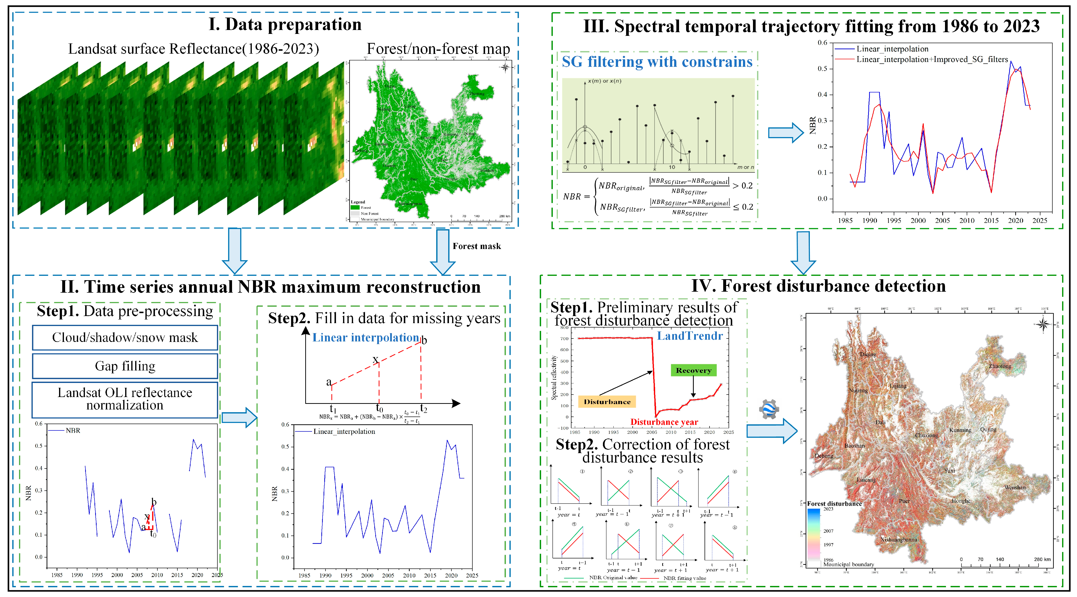
3.1. Reconstruction of High-Density Landsat Time-Series Data

The time series of the maximum-value composite NBR data from January to April was utilized to monitor forest disturbances. However, Yunnan Province’s complex terrain and climatic variability make the spatial distribution of high-quality, cloud-free Landsat images uneven. This has resulted in substantial discrepancies in the cumulative years of Landsat data across different regions, leading to data gaps in certain areas. To generate a complete and continuous NBR time series from 1986 to 2023, linear interpolation [68] was employed to estimate the NBR values for the missing years. Specifically, the NBR value for a missing year was predicted using a linear relationship based on the two adjacent years with available data, as calculated by the following equation:

$${\mathrm{NBR}}_{\mathrm{x}}={\mathrm{NBR}}_{\mathrm{a}}+\left({\mathrm{NBR}}_{\mathrm{b}}-{\mathrm{NBR}}_{\mathrm{a}}\right)\times {\displaystyle \frac{{\mathrm{t}}_0-{\mathrm{t}}_1}{{\mathrm{t}}_2-{\mathrm{t}}_1}}$$

(2)

where ${\mathrm{NBR}}_{\mathrm{x}}$ is the estimated NBR value for the missing year; ${\mathrm{t}}_1$ and ${\mathrm{t}}_2$ are the years with available, high-quality Landsat data before and after the missing year; and ${\mathrm{NBR}}_{\mathrm{a}}$ and ${\mathrm{NBR}}_{\mathrm{b}}$ are the observed NBR values for the years ${\mathrm{t}}_1$ and ${\mathrm{t}}_2$, respectively.

3.2. Spectral Time-Series Trajectory Fitting

Although the SG filter can effectively remove residual noise while preserving the overall trend in the NBR time-series data [69], balancing data smoothing and maintaining the true change trends becomes challenging when abrupt signals are present in multi-temporal data [28]. The core of the SG filter involves weighted filtering within a sliding window, where the weights are derived from the ordinary least squares fit of a high-order polynomial to the NBR data in that window. However, abrupt forest disturbance events, such as forest fires, pest outbreaks, and deforestation, do not conform to the assumptions of polynomial fitting. As a result, SG-filtered trajectories for such abrupt disturbances often deviate significantly from reality (Figure 5a). For example, the visually interpreted forest disturbance year based on satellite observation is 2015, whereas the SG-filter-generated trajectory detects the disturbance in 2014.

To address this issue, a constrained SG filtering algorithm was proposed in this study to refine the NBR temporal trajectory for abrupt forest disturbance events. Specifically, when the absolute rate of change between the NBR value collected by satellite observation and that estimated by the SG filter exceeds a certain threshold, the satellite-observed NBR value replaces the SG-filtered value for that year. If the change rate remains below the threshold, the SG-filtered value is retained. As shown in Figure 5, the spectral trajectory produced by the constrained SG filter algorithm more accurately reflects the disturbance trends and aligns closely with actual observations. The constrained SG filtering algorithm is expressed as follows:

$$\mathrm{NBR}=\left\{\begin{array}{c}{\mathrm{NBR}}_{\mathrm{original}}, {\displaystyle \frac{\left|{\mathrm{NBR}}_{\mathrm{SGfilter}}-{\mathrm{NBR}}_{\mathrm{original}}\right|}{{\mathrm{NBR}}_{\mathrm{SGfilter}}}}>\mathrm{t}\mathrm{h}\mathrm{r}\mathrm{e}\mathrm{s}\mathrm{h}\mathrm{o}\mathrm{l}\mathrm{d} \\ {\mathrm{NBR}}_{\mathrm{SGfilter}}, {\displaystyle \frac{\left|{\mathrm{NBR}}_{\mathrm{SGfilter}}-{\mathrm{NBR}}_{\mathrm{original}}\right|}{{\mathrm{NBR}}_{\mathrm{SGfilter}}}}\le \mathrm{t}\mathrm{h}\mathrm{r}\mathrm{e}\mathrm{s}\mathrm{h}\mathrm{o}\mathrm{l}\mathrm{d} \end{array}\right.$$

(3)

where $\mathrm{NBR}$ denotes the NBR value for each year; ${\mathrm{NBR}}_{\mathrm{original}}$ and ${\mathrm{NBR}}_{\mathrm{SGfilter}}$ are the NBR values derived from satellite observation and SG filter, respectively; and the $\mathrm{threshold}$ is the regimentation threshold, which was defined as 0.2.

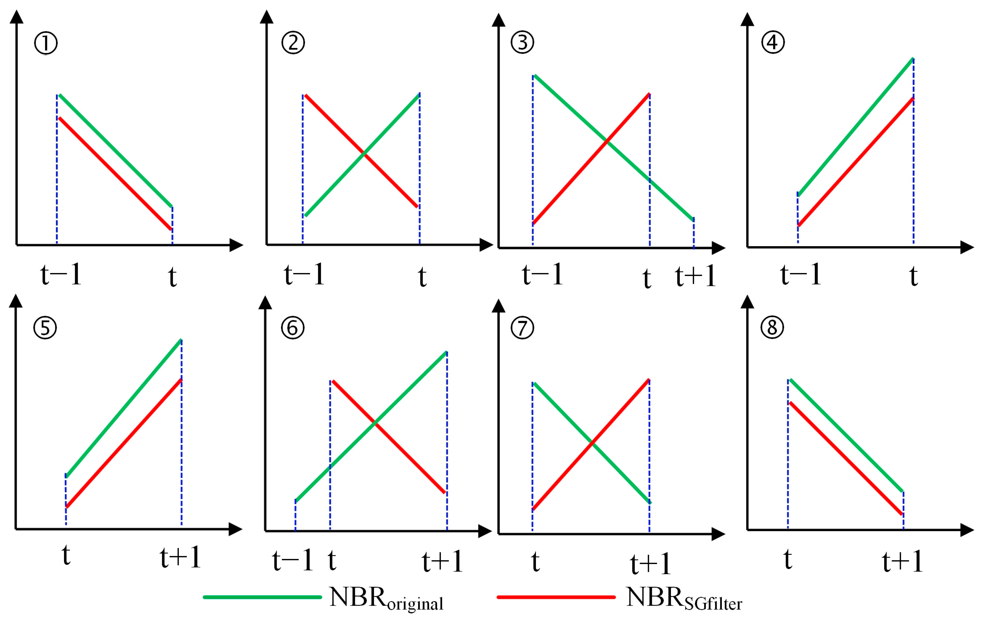
3.3. Forest Disturbance Detection

The preliminary results of forest disturbance detection were generated using the LandTrendr algorithms [70]. The results were subsequently corrected by comparing the NBR time-series trajectories fitted from satellite observations with those from the constrained SG filter. Figure 6 illustrates eight scenarios depicting the changes in spectral indices between the detected disturbance year and the adjacent years. When the spectral trajectories derived from the satellite observations and the constrained SG filter align (i.e., scenarios ① and ⑤), the disturbance year detected by LandTrendr is considered accurate and should be retained. Conversely, if the NBR value in the disturbance year from the satellite observations is higher than that of the previous year (i.e., scenarios ②, ④, and ⑥), it indicates that the disturbance year detected by LandTrendr is delayed, suggesting that the actual disturbance occurred in the previous year. Additionally, if the NBR values in the disturbance year from the satellite observations are lower than those in the following year (i.e., scenarios ③, ⑦, and ⑧), it implies that the true disturbance year should be the year following the one detected by LandTrendr. This correction is expressed mathematically in Equation (4):

$$\mathrm{Disturbance} \mathrm{year}=\left\{\begin{array}{c}\mathrm{t}, \mathrm{condition}:➀,➄ \\ \mathrm{t}+1, \mathrm{condition}:➂,➆,➇\\ \mathrm{t}-1,\mathrm{condition}:➁,➃,➅\end{array}\right.$$

(4)

where the $\mathrm{Disturbance} \mathrm{year}$ denotes the corrected year of forest disturbance, $\mathrm{t}$ is the disturbance year detected by the LandTrendr algorithm, and the $\mathrm{condition}$ refers to the scenarios depicted in Figure 6.

3.4. Accuracy Assessment

The validation samples from three sources were used to quantitatively assess the effectiveness of the iLandTrendr algorithm for forest disturbance mapping. Four widely recognized indices, the overall accuracy (OA), omission error (OE), commission error (CE), and F1 score were used to quantify the mapping accuracy. A higher value of the OA and F1 score represented the method having a better performance for forest disturbance mapping. On the contrary, the smaller value of OE and CE indicates that the method is more effective in detecting complex forest disturbance types. These indices are given as the following equation:

$$\mathrm{OA}={\displaystyle \frac{\mathrm{n}}{\mathrm{N}}}\times 100\%$$

(5)

$$\mathrm{CE}={\displaystyle \frac{\mathrm{b}}{\mathrm{B}}}\times 100\%$$

(6)

$$\mathrm{OE}={\displaystyle \frac{\mathrm{d}}{\mathrm{D}}}\times 100\%$$

(7)

$$\mathrm{F}1 \mathrm{score}={\displaystyle \frac{\left(1-\mathrm{CE}\right)\times \left(1-\mathrm{OE}\right)}{\left(2-\mathrm{CE}-\mathrm{OE}\right)}}\times 200\%$$

(8)

where $\mathrm{n}$ represents the number of pixels correctly detected as disturbed; $\mathrm{b}$ is the total number of pixels incorrectly detected; $\mathrm{d}$ is the number of pixels missed by the model, that is, the area where the disturbance occurred but was not detected; $\mathrm{B}$ and $\mathrm{D}$ are the total numbers of pixels with and without forest disturbance in the validation sample, respectively; and $\mathrm{N}$ is the total number of validation samples, with $\mathrm{N}=\mathrm{B}+\mathrm{D}$.

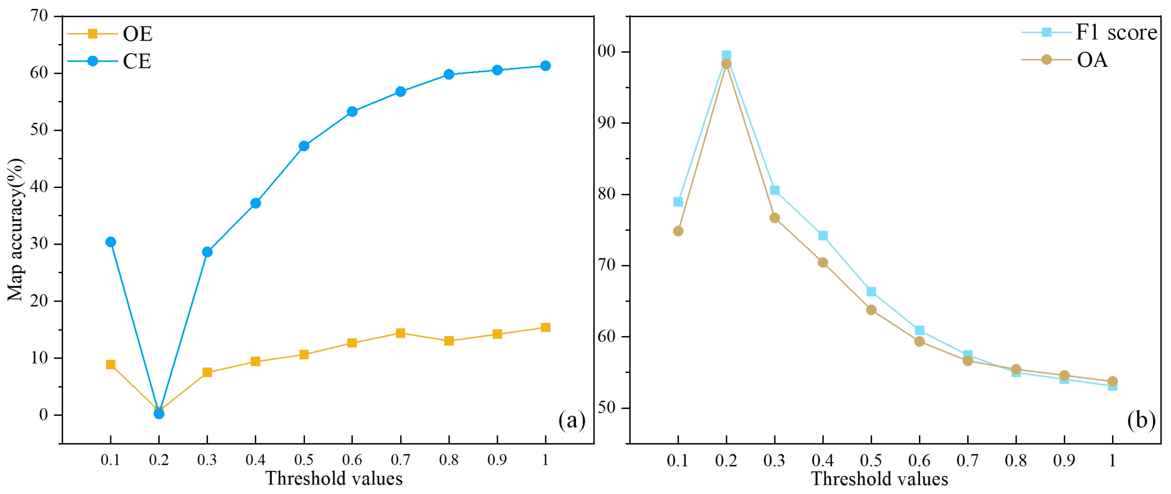
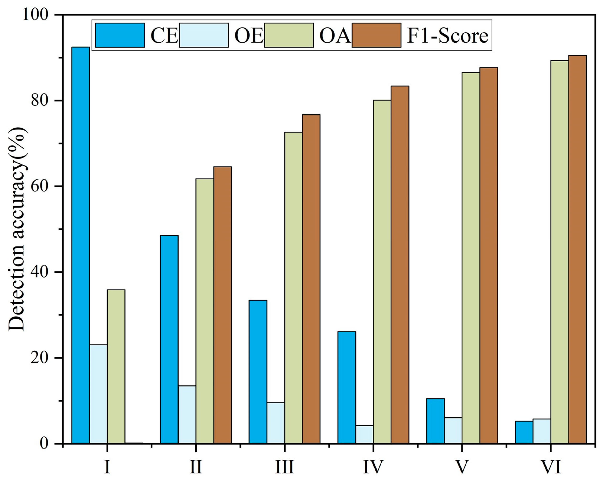
3.5. Experiment Design

To quantitatively evaluate the effectiveness of the iLandTrendr algorithm proposed in this study for forest disturbance mapping, six experimental schemes (

Table 3. Combination of input parameters in the experiment.

Experimental Schemes	Description
I	NBR time-series data from June to September + Sliding window method
II	NBR time-series data from January to April + Sliding window method
III	NBR time-series data from January to April + Linear interpolation method
IV	NBR time-series data from January to April + Linear interpolation method + SG filter
V	NBR time-series data from January to April + Linear interpolation method + Constrained SG filter
VI	NBR time-series data from January to April + Linear interpolation method + Constrained SG filter + Correction of forest disturbance detection results

) were designed, and their detection accuracy was assessed using the validation samples. These experimental schemes were primarily aimed at evaluating the accuracy of forest disturbance detection based on Landsat time-series data reconstruction, spectral trajectory fitting, and result correction.

Schemes I and II were employed to assess the impact of the seasonal Landsat composite data on forest disturbance detection in cloudy and rainy regions. Schemes II and III were used to evaluate the effects of various data-filling methods on the detection results. Furthermore, schemes IV and V were implemented to examine the contribution of the constrained SG filter algorithm to forest disturbance detection. Finally, schemes V and VI were used to assess the effectiveness of the post-processing steps applied to the forest disturbance detection results generated by the LandTrendr algorithm. All the experiments were conducted using the GEE platform, with the optimal threshold parameters for the LandTrendr algorithm from [70] applied for the forest disturbance mapping.

4. Results

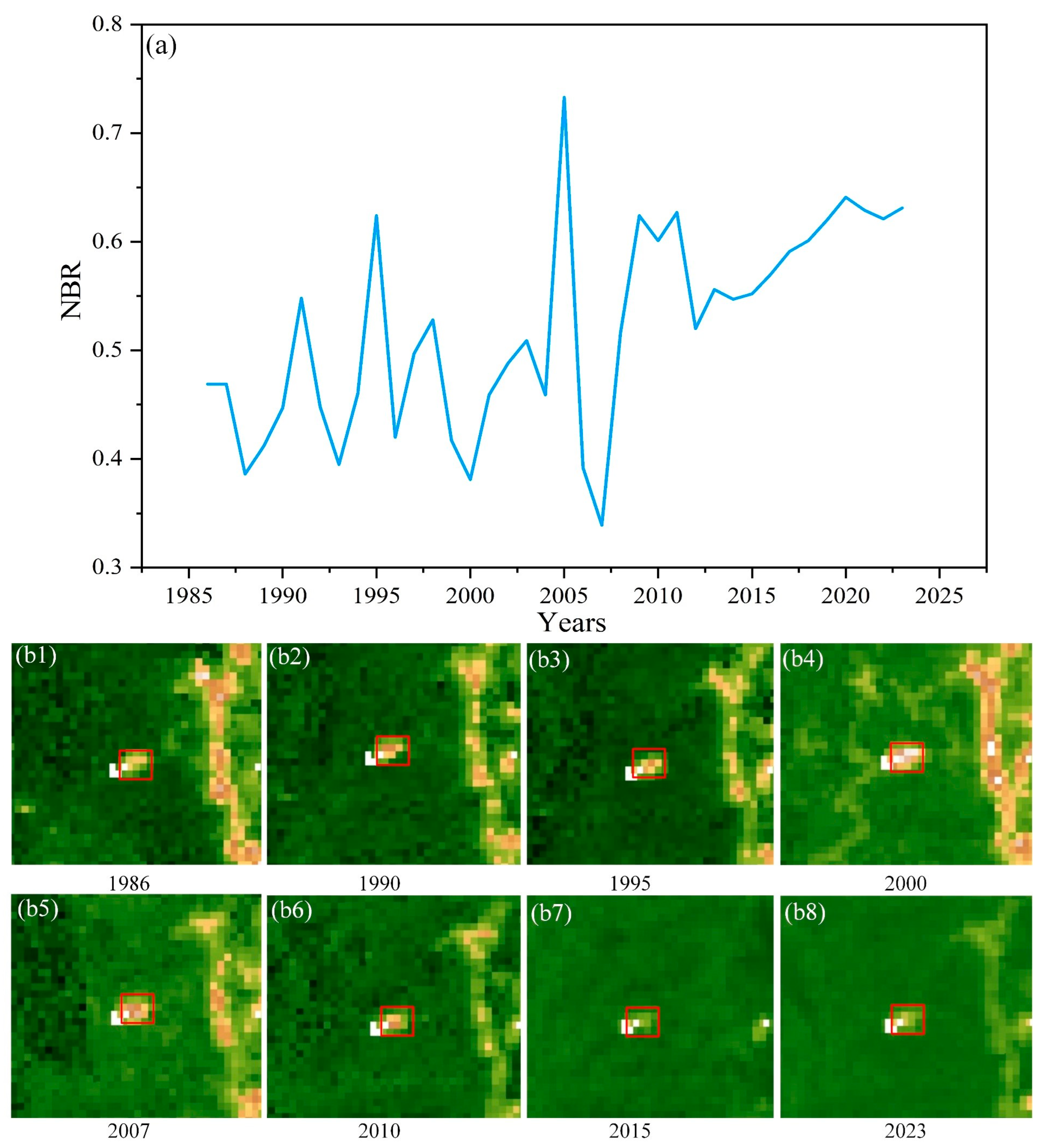
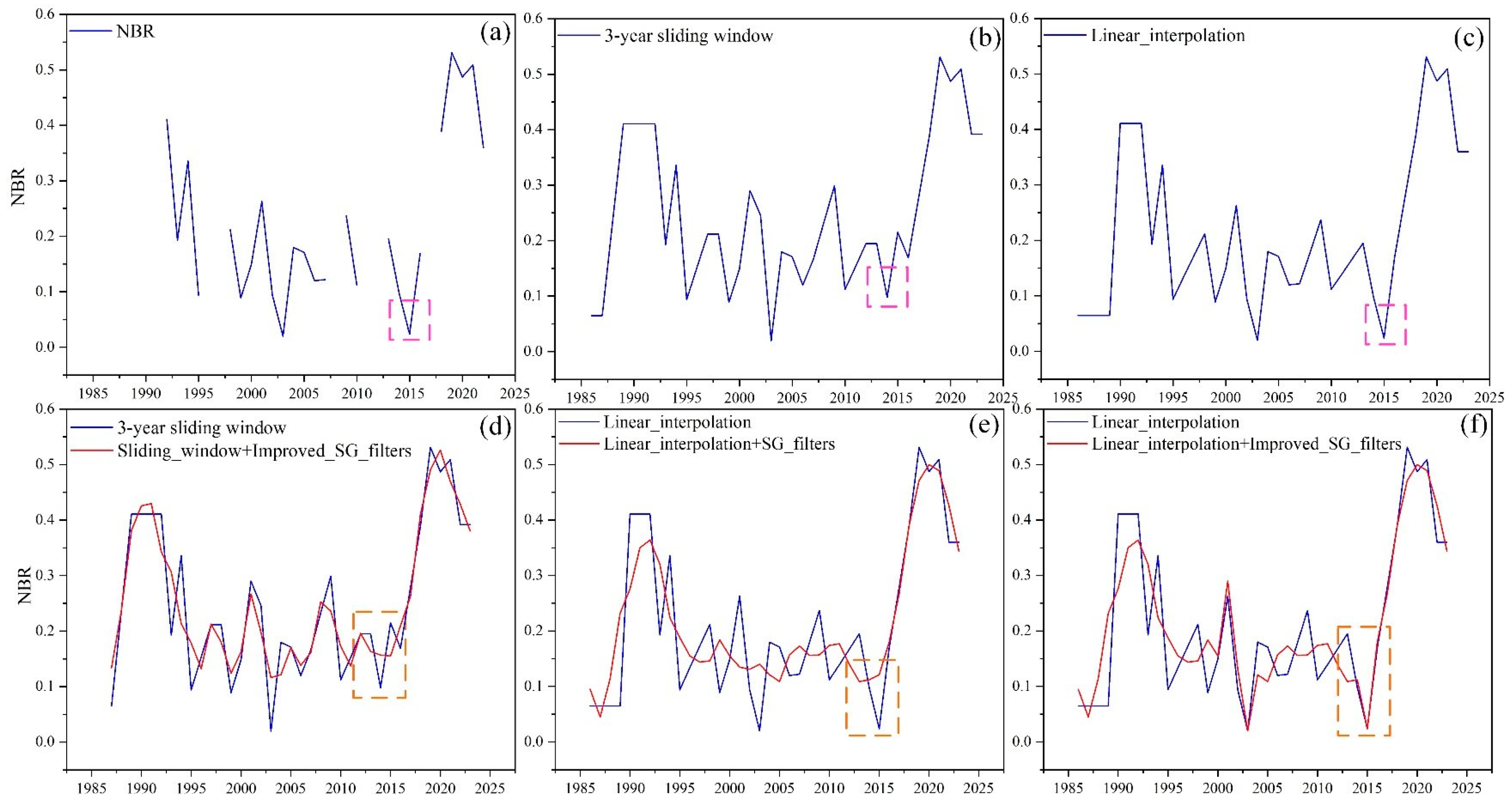
4.1. Evaluating the Quality of Temporal Trajectory

The quality of the temporal trajectory for complex forest disturbance types is crucial for accurate forest disturbance mapping [71]. To assess the effectiveness of the various data filling and fitting methods for generating these temporal trajectories, a pixel of the forest fire in Yuxi, Yunnan Province, in 2015 was selected for verification (Figure 7). The experimental results demonstrated that the NBR time-series data reconstructed using the sliding window method did not align well with the actual observed values from 2015 (Figure 7b). In contrast, the NBR time series filled using linear interpolation better preserved the true change information from the satellite observations (Figure 7c). When compared with the NBR temporal trajectory generated by the constrained SG filter (Figure 7f), the trajectory fitted by the original SG filter exhibited a pseudo-change from 2013 to 2015 (Figure 7e). Specifically, the original NBR trajectory showed a downward trend, while the trajectory after fitting showed an upward trend. This discrepancy in spectral change could have led the LandTrendr algorithm to incorrectly identify the forest disturbance year for the pixel as 2014. Additionally, the NBR temporal trajectory produced by the sliding window method and constrained SG filter contained pseudo-change information from 2010 to 2011 (Figure 7d), potentially causing the LandTrendr algorithm to detect the disturbance year as 2011.

Therefore, the spectral time-series trajectory generated by the linear interpolation method and constrained SG filter closely approximated the actual spectral trajectory for abrupt forest disturbances like forest fires, thereby significantly improving the detection accuracy for the complex forest disturbance types.

In addition, obtaining the optimal constraints for the SG filter plays an important role in generating the accurate temporal trajectories of complex forest disturbance types [44]. In this study, the constraint threshold was set from 0.1 to 1 with an increment of 0.1. The OA and F1 scores for the forest disturbance mapping at different constraint thresholds, as tested in the parameter sensitivity experiment, are presented in Figure 8. The results showed that as the constraint threshold increased, the CE and OE of forest disturbance detection in Yunnan Province showed a changing trend of initially decreasing, then increasing (Figure 8a). At a constraint threshold of 0.2, OE and CE reached their lowest values, 5.75% and 5.25%, respectively. Similarly, the detection accuracy for forest disturbances using the constrained SG filter followed a trend of initial improvement, followed by a decline (Figure 8b). At a threshold of 0.2, the detection accuracy was at its highest, with the OA and F1 scores of 89.32% and 90.50%, respectively. Therefore, a threshold of 0.2 yielded the highest detection accuracy for complex forest disturbances using the iLandTrendr algorithm proposed in this study. This threshold likely preserved the key satellite observations of critical time points during the forest disturbance events, resulting in NBR temporal trajectories that closely matched the actual conditions of forest disturbances.

4.2. Evaluating the Effectiveness of the iLandTrendr Algorithm for Forest Disturbance Mapping

Figure 9 and

Table 4. Accuracy assessment of forest disturbance detection in different experimental schemes.

	CE (%)	OE (%)	OA (%)	F1 Score (%)
I	92.46	23.08	35.88	13.73
II	48.49	13.50	61.73	64.57
III	33.42	9.56	72.62	76.70
IV	26.13	4.23	80.1	83.40
V	10.52	6.05	86.58	87.66
VI	5.25	5.75	89.32	90.50

show that the iLandTrendr algorithm is effective for forest disturbance mapping over large areas. First, the NBR time-series data composited from January to April significantly improved mapping accuracy in cloudy and rainy regions. Compared to the NBR time-series data from the vegetation growing season (June to September), the F1 score and OA increased by 50.80 and 25.85%, respectively, while CE and OE decreased by 43.97 and 9.58%, respectively. Second, the use of linear interpolation to fill in missing NBR data from certain years allowed for the generation of a complete and continuous NBR time series from 1986 to 2023. This approach effectively improved mapping accuracy in regions with consistently missing high-quality Landsat images. Compared to the sliding average method for filling missing years, the F1 score and OA increased by 12.10% and 10.89%, respectively, and CE and OE decreased by 15.07% and 3.94%. Third, the constrained SG filter better preserved the spectral information of critical time points during abrupt forest disturbance events, leading to enhanced detection accuracy for complex disturbance types. Compared to the original SG filter, the F1 score and OA increased by 6.48% and 4.26%, respectively, while CE and OE decreased by 15.61% and 1.82%. Finally, when compared to the original LandTrendr algorithm, the difference between the spectral trajectories fitted from the satellite observations and constrained SG filtering effectively improved the detection accuracy of the complex forest disturbance types, with the F1 score and OA increasing by 2.84% and 2.74%, and CE and OE decreasing by 5.27% and 0.30%, respectively. In summary, the iLandTrendr algorithm demonstrated a significant improvement in detecting complex forest disturbances over the original LandTrendr algorithm, with the F1 score and OA increasing by 76.77% and 53.44%, respectively, and CE and OE decreasing by 87.21% and 17.33%. These results indicate that the iLandTrendr algorithm effectively preserves complete and reliable spectral trajectories, thereby enhancing the accuracy of forest disturbance detection.

4.3. Spatiotemporal Characteristics of Forest Disturbance in Yunnan Province from 1986 to 2023

Following the procedure described in Section 3, forest disturbance mapping at a 30 m resolution across Yunnan Province was conducted using the iLandTrendr algorithm (Figure 10). The results demonstrated that forest disturbance in the study area was relatively severe. From 1986 to 2023, the total disturbed forest area was approximately 1,985,820.9 km², accounting for 49.69% of the province’s total area. Among the disturbance years, 1986 had the largest disturbed area (15,498.11 km²), representing 3.93% of the total disturbance area, while 2022 had the smallest disturbed area (315.66 km²), accounting for only 0.08% (Figure 11a). Meanwhile, the year of forest disturbance shows a significant spatial heterogeneity in Yunnan Province. For example, disturbances in the northwest predominantly occurred during the 1990s, and the primary land cover change was from forest to cultivated land [72]. In contrast, the forest disturbances in southern tropical regions such as Xishuangbanna, Pu’er, and Dehong were largely concentrated during the period of extensive rubber plantation development (2000–2015), where natural forests were primarily converted into rubber plantations [49]. Due to the implementation of national policies such as returning farmland to forests, the establishment of nature reserves, and forest protection and utilization programs, the area of forest disturbance has steadily declined since 2010.

In addition, there is significant spatial heterogeneity in the intensity of forest disturbance across Yunnan Province (Figure 11). First, forest disturbances were most intense in the regions at elevations between 1000 and 2000 m, accounting for 76.26% of the total disturbed area, while the disturbances at elevations above 3000 m were minimal, comprising only 6.44% (Figure 11b). The timing of disturbances also varied with elevation: 17.07% of the disturbances below 1000 m occurred between 2007 and 2012, whereas 57.96% of the disturbances above 1000 m took place from 1987 to 2002. Second, as the mean annual temperature increased, disturbance intensity first increased and then decreased (Figure 11c). The highest intensity was observed in the regions with mean annual temperatures between 6 and 11 °C, accounting for 76.42% of the disturbed area. Most disturbances in these temperature regions occurred from 1987 to 2002, representing 56.63% of the total disturbed area. Finally, a positive correlation was found between disturbance intensity and mean annual precipitation (Figure 11d). The highest disturbance intensity occurred in regions with mean annual precipitation above 1220 mm, constituting 77.19% of the disturbed area. Over time, the disturbance intensity in these precipitation regions showed a decreasing trend, with 54.82% of the disturbances occurring between 1987 and 2002. In summary, the highest forest disturbance intensity was observed in the areas with elevations between 2000 and 3000 m, mean annual temperatures between 6 and 11 °C, and mean annual precipitation above 1220 mm, accounting for 76.26%, 76.42%, and 77.19% of the disturbed area, respectively. Most forest disturbances occurred from 1987 to 2002, with this period contributing 56.47% of the total disturbed area.

4.4. Attribution Analysis of Forest Disturbance

The forest disturbance agents in Yunnan Province were classified using the RF algorithm [73,74] based on terrain features (elevation, slope, and aspect) and the yearly composited Landsat imagery from 1986 to 2023 (Figure 12). The results showed that there was a significant spatial agglomeration effect in the attribution of the forest disturbance agents. For example, forest fires, often difficult to extinguish due to the high amount of combustible material in forested areas, were predominantly distributed in patchy patterns [75]. Similarly, the deforestation events were concentrated in the urban fringes and low-latitude areas of Xishuangbanna, where rubber plantations are prevalent [76]. In these areas, land use primarily converted from forests to agricultural land and impervious surfaces [77]. Additionally, forest diseases and insect infestations were mainly observed in natural forests at higher altitudes. This could be attributed to the high tree density, uniform growth patterns, poor forest development, and reduced resistance to diseases and pests in these regions. Forest degradation was primarily concentrated in southern areas such as Xishuangbanna, Honghe, and Lincang, which have abundant water and heat. This phenomenon may be driven by large-scale economic forest planting and the rapid growth of tourism, both of which have exacerbated ecological pressures in these regions. Pests and diseases were found to be the primary drivers of forest disturbance in Yunnan Province, accounting for 37.49% of the total disturbance area, followed by forest degradation (32.23%), forest fires (15.59%), and deforestation (14.49%). In conclusion, the forest disturbances in Yunnan Province were influenced by both natural and anthropogenic factors, with the natural factors playing a more prominent interactive role.

5. Discussions

Detecting forest disturbance is essential for sustainable forest management. Although LandTrendr is one of the widely used algorithms for forest disturbance mapping, it still has two limitations that may hinder its effectiveness in large-scale applications. First, it employs a uniform SG filter [38] to remove data noise from multi-temporal Landsat data and fit the temporal trajectory of the complex forest disturbance types, which may introduce uncertainties in forest disturbance mapping. Second, the fixed model parameters are used to detect all the forest disturbance types, which may reduce the mapping accuracy for certain forest disturbance types [40,41]. This paper focused on improving LandTrendr for forest disturbance mapping in the two mentioned aspects by optimizing temporal trajectories and applying post-processing to the detection results. Specifically, a constrained SG filter was applied to optimize the temporal trajectory for the complex forest disturbance types. Additionally, the forest disturbances detected by LandTrendr were further modified using the consistency of the spectral index change trends. With these improvements, the OA of forest disturbance detection in Yunnan Province increased from 35.88 to 89.32% (Table 4).

In addition, the forest disturbance mapping developed by iLandTrendr was compared to a Global Forest gain and loss product at 30 m spatial resolution [78]. To keep consistency, the forest loss from 2001 to 2023 was used for comparison in this paper. The OA, F1 score, OE, and CE of Hansen’s product [78] achieved 55.77%, 62.30%, 24.00%, and 47.22%, respectively. These values were 34.55% and 28.20% lower than the OA and F1 score of iLandTrendr, respectively.

The above results demonstrate that the proposed iLandTrendr algorithm has greater effectiveness for forest disturbance mapping, but it also has certain limitations. First, the iLandTrendr only used yearly Landsat composited data from January to April to monitor forest disturbance, which may delay detected forest disturbance that occurred from May to December by one year. The integration of satellite observations from multi-season may further improve the accuracy of iLandTrendr for forest disturbance mapping [46]. Second, the NBR is a commonly used spectral index in forest disturbance mapping due to its high sensitivity to forest disturbance and recovery [35,45,46]. However, only a single spectral index (NBR) was used in iLandTrendr to detect all the forest disturbance types, which may introduce the uncertainty of certain forest disturbance types. Previous studies [45,46] have shown that there are significant differences in the optimal forest disturbance monitoring indicators and segmentation thresholds for different regions of forest types. Therefore, the effectiveness of the iLandTrendr algorithm for forest disturbance mapping may be further improved by adaptively selecting monitoring indicators and calibrating optimal thresholds for each parameter.

6. Conclusions

In this study, we improved the LandTrendr algorithm (iLandtrendr) for forest disturbance mapping by optimizing the temporal trajectories of the spectral index and applying post-processing to the detection results. It used the constraint SG filter to preserve the important spectral change information associated with the complex forest disturbance types. The forest disturbance detected by LandTrendr at each pixel has been further modified using the consistency of spectral index trends, fitted by the constrained SG filter and satellite observations. The iLandtrendr algorithm was calibrated and validated using a set of validated samples in Yunnan Province based on the Landsat time series data from 1986 to 2023. With these two improvements, the accuracy of forest disturbance mapping across Yunnan Province increased significantly, with the overall accuracy increasing by 53.44%. The iLandtrendr algorithm can accurately detect the year of complex forest disturbance occurrence and has the potential to be applied at national and global scales for forest disturbance mapping. However, the quality of optical remote-sensing images is often affected by weather conditions. Future research should focus on enhancing detection accuracy for complex forest disturbance types by integrating optical and microwave radar imagery, which is less affected by weather.

References

1. Seidl, R.; Thom, D.; Kautz, M.; Martin-Benito, D.; Peltoniemi, M.; Vacchiano, G.; Wild, J.; Ascoli, D.; Petr, M.; Honkaniemi, J.; et al. Forest disturbances under climate change. Nat. Clim. Chang. 2017, 7, 395–402. [Google Scholar] [CrossRef] [PubMed]
2. Cannon, J.B.; Peterson, C.J.; O’Brien, J.J.; Brewer, J.S. A review and classification of interactions between forest disturbance from wind and fire. For. Ecol. Manag. 2017, 406, 381–390. [Google Scholar] [CrossRef]
3. van Lierop, P.; Lindquist, E.; Sathyapala, S.; Franceschini, G. Global forest area disturbance from fire, insect pests, diseases and severe weather events. For. Ecol. Manag. 2015, 352, 78–88. [Google Scholar] [CrossRef]
4. Santos, A.M.D.; Silva, C.; Almeida Junior, P.M.; Rudke, A.P.; Melo, S.N. Deforestation drivers in the Brazilian Amazon: Assessing new spatial predictors. J. Environ. Manag. 2021, 294, 113020. [Google Scholar] [CrossRef]
5. Pennington, D.N.; Hansel, J.R.; Gorchov, D.L. Urbanization and riparian forest woody communities: Diversity, composition, and structure within a metropolitan landscape. Biol. Conserv. 2010, 143, 182–194. [Google Scholar] [CrossRef]
6. Trigueiro, W.R.; Nabout, J.C.; Tessarolo, G. Uncovering the spatial variability of recent deforestation drivers in the Brazilian Cerrado. J. Environ. Manag. 2020, 275, 111243. [Google Scholar] [CrossRef]
7. da Silva, C.F.A.; Dos Santos, A.M.; de Melo, S.N.; Rudke, A.P.; de Almeida Junior, P.M. Spatial modelling of deforestation-related factors in the Brazilian semi-arid biome. Int. J. Environ. Stud. 2023, 80, 1021–1040. [Google Scholar] [CrossRef]
8. Qi, J.-H.; Fan, Z.-X.; Fu, P.-L.; Zhang, Y.-J.; Sterck, F.; Mencuccini, M. Differential determinants of growth rates in subtropical evergreen and deciduous juvenile trees: Carbon gain, hydraulics and nutrient-use efficiencies. Tree Physiol. 2021, 41, 12–23. [Google Scholar] [CrossRef]
9. Seidl, R.; Schelhaas, M.J.; Rammer, W.; Verkerk, P.J. Increasing forest disturbances in Europe and their impact on carbon storage. Nat. Clim. Chang. 2014, 4, 806–810. [Google Scholar] [CrossRef]
10. Espirito-Santo, F.D.; Gloor, M.; Keller, M.; Malhi, Y.; Saatchi, S.; Nelson, B.; Junior, R.C.; Pereira, C.; Lloyd, J.; Frolking, S.; et al. Size and frequency of natural forest disturbances and the Amazon forest carbon balance. Nat. Commun. 2014, 5, 3434. [Google Scholar] [CrossRef]
11. Shang, R.; Chen, J.M.; Xu, M.; Lin, X.; Li, P.; Yu, G.; He, N.; Xu, L.; Gong, P.; Liu, L.; et al. China’s current forest age structure will lead to weakened carbon sinks in the near future. Innovation 2023, 4, 100515. [Google Scholar] [CrossRef]
12. Sun, R.; Zhao, F.; Huang, C.; Huang, H.; Lu, Z.; Zhao, P.; Ni, X.; Meng, R. Integration of deep learning algorithms with a Bayesian method for improved characterization of tropical deforestation frontiers using Sentinel-1 SAR imagery. Remote Sens. Environ. 2023, 298, 113821. [Google Scholar] [CrossRef]
13. Pflugmacher, D.; Cohen, W.B.; Kennedy, R.E. Using Landsat-derived disturbance history (1972–2010) to predict current forest structure. Remote Sens. Environ. 2012, 122, 146–165. [Google Scholar] [CrossRef]
14. Lu, D.; Mausel, P.; Brondízio, E.; Moran, E. Change detection techniques. Int. J. Remote Sens. 2010, 25, 2365–2401. [Google Scholar] [CrossRef]
15. Verbesselt, J.; Hyndman, R.; Newnham, G.; Culvenor, D. Detecting trend and seasonal changes in satellite image time series. Remote Sens. Environ. 2010, 114, 106–115. [Google Scholar] [CrossRef]
16. Seidl, R.; Fernandes, P.M.; Fonseca, T.F.; Gillet, F.; Jönsson, A.M.; Merganičová, K.; Netherer, S.; Arpaci, A.; Bontemps, J.-D.; Bugmann, H.; et al. Modelling natural disturbances in forest ecosystems: A review. Ecol. Model. 2011, 222, 903–924. [Google Scholar] [CrossRef]
17. Griffiths, P.; Kuemmerle, T.; Baumann, M.; Radeloff, V.C.; Abrudan, I.V.; Lieskovsky, J.; Munteanu, C.; Ostapowicz, K.; Hostert, P. Forest disturbances, forest recovery, and changes in forest types across the Carpathian ecoregion from 1985 to 2010 based on Landsat image composites. Remote Sens. Environ. 2014, 151, 72–88. [Google Scholar] [CrossRef]
18. DeVries, B.; Verbesselt, J.; Kooistra, L.; Herold, M. Robust monitoring of small-scale forest disturbances in a tropical montane forest using Landsat time series. Remote Sens. Environ. 2015, 161, 107–121. [Google Scholar] [CrossRef]
19. Malila, W.A. Change vector analysis: An approach for detecting forest changes with Landsat. In Proceedings of the LARS symposia, West Lafayette, IN, USA, 3–6 June 1980; p. 385. [Google Scholar]
20. Healey, S.; Cohen, W.; Zhiqiang, Y.; Krankina, O. Comparison of Tasseled Cap-based Landsat data structures for use in forest disturbance detection. Remote Sens. Environ. 2005, 97, 301–310. [Google Scholar] [CrossRef]
21. Shimada, M.; Itoh, T.; Motooka, T.; Watanabe, M.; Shiraishi, T.; Thapa, R.; Lucas, R. New global forest/non-forest maps from ALOS PALSAR data (2007–2010). Remote Sens. Environ. 2014, 155, 13–31. [Google Scholar] [CrossRef]
22. Lv, Z.Y.; Liu, T.F.; Zhang, P.; Benediktsson, J.A.; Lei, T.; Zhang, X. Novel Adaptive Histogram Trend Similarity Approach for Land Cover Change Detection by Using Bitemporal Very-High-Resolution Remote Sensing Images. IEEE Trans. Geosci. Remote Sens. 2019, 57, 9554–9574. [Google Scholar] [CrossRef]
23. Zhang, Y.; Wang, L.; Zhou, Q.; Tang, F.; Zhang, B.; Huang, N.; Nath, B. Continuous Change Detection and Classification—Spectral Trajectory Breakpoint Recognition for Forest Monitoring. Land 2022, 11, 504. [Google Scholar] [CrossRef]
24. Wang, Z.; Wei, C.; Liu, X.; Zhu, L.; Yang, Q.; Wang, Q.; Zhang, Q.; Meng, Y. Object-based change detection for vegetation disturbance and recovery using Landsat time series. GIScience Remote Sens. 2022, 59, 1706–1721. [Google Scholar] [CrossRef]
25. DeVries, B.; Decuyper, M.; Verbesselt, J.; Zeileis, A.; Herold, M.; Joseph, S. Tracking disturbance-regrowth dynamics in tropical forests using structural change detection and Landsat time series. Remote Sens. Environ. 2015, 169, 320–334. [Google Scholar] [CrossRef]
26. Zhu, Z.; Woodcock, C.E. Continuous change detection and classification of land cover using all available Landsat data. Remote Sens. Environ. 2014, 144, 152–171. [Google Scholar] [CrossRef]
27. Zhu, Z.; Zhang, J.; Yang, Z.; Aljaddani, A.H.; Cohen, W.B.; Qiu, S.; Zhou, C. Continuous monitoring of land disturbance based on Landsat time series. Remote Sens. Environ. 2020, 238, 111116. [Google Scholar] [CrossRef]
28. Zhu, Z.; Woodcock, C.E.; Olofsson, P. Continuous monitoring of forest disturbance using all available Landsat imagery. Remote Sens. Environ. 2012, 122, 75–91. [Google Scholar] [CrossRef]
29. Yin, H.; Prishchepov, A.V.; Kuemmerle, T.; Bleyhl, B.; Buchner, J.; Radeloff, V.C. Mapping agricultural land abandonment from spatial and temporal segmentation of Landsat time series. Remote Sens. Environ. 2018, 210, 12–24. [Google Scholar] [CrossRef]
30. Kennedy, R.E.; Cohen, W.B.; Schroeder, T.A. Trajectory-based change detection for automated characterization of forest disturbance dynamics. Remote Sens. Environ. 2007, 110, 370–386. [Google Scholar] [CrossRef]
31. Shen, J.; Chen, G.; Hua, J.; Huang, S.; Ma, J. Contrasting Forest Loss and Gain Patterns in Subtropical China Detected Using an Integrated LandTrendr and Machine-Learning Method. Remote Sens. 2022, 14, 3238. [Google Scholar] [CrossRef]
32. Kennedy, R.E.; Yang, Z.; Cohen, W.B. Detecting trends in forest disturbance and recovery using yearly Landsat time series: 1. LandTrendr—Temporal segmentation algorithms. Remote Sens. Environ. 2010, 114, 2897–2910. [Google Scholar] [CrossRef]
33. Cohen, W.B.; Yang, Z.; Healey, S.P.; Kennedy, R.E.; Gorelick, N. A LandTrendr multispectral ensemble for forest disturbance detection. Remote Sens. Environ. 2018, 205, 131–140. [Google Scholar] [CrossRef]
34. Nasirzadehdizaji, R.; Balik Sanli, F.; Abdikan, S.; Cakir, Z.; Sekertekin, A.; Ustuner, M. Sensitivity Analysis of Multi-Temporal Sentinel-1 SAR Parameters to Crop Height and Canopy Coverage. Appl. Sci. 2019, 9, 655. [Google Scholar] [CrossRef]
35. Li, Y.; Wu, Z.; Xu, X.; Fan, H.; Tong, X.; Liu, J. Forest disturbances and the attribution derived from yearly Landsat time series over 1990–2020 in the Hengduan Mountains Region of Southwest China. For. Ecosyst. 2021, 8, 73. [Google Scholar] [CrossRef]
36. Kennedy, R.; Yang, Z.; Gorelick, N.; Braaten, J.; Cavalcante, L.; Cohen, W.; Healey, S. Implementation of the LandTrendr Algorithm on Google Earth Engine. Remote Sens. 2018, 10, 691. [Google Scholar] [CrossRef]
37. Danylo, O.; Pirker, J.; Lemoine, G.; Ceccherini, G.; See, L.; McCallum, I.; Hadi; Kraxner, F.; Achard, F.; Fritz, S. A map of the extent and year of detection of oil palm plantations in Indonesia, Malaysia and Thailand. Sci. Data 2021, 8, 96. [Google Scholar] [CrossRef]
38. Press, W.H.; Teukolsky, S.A. Savitzky-Golay Smoothing Filters. Comput. Phys. 1990, 4, 669–672. [Google Scholar] [CrossRef]
39. Seron, M.M.; Braslavsky, J.H.; Goodwin, G.C. Fundamental Limitations in Filtering and Control; Springer Science & Business Media: Berlin/Heidelberg, Germany, 2012. [Google Scholar]
40. Zhu, L.; Liu, X.; Wu, L.; Tang, Y.; Meng, Y. Long-Term Monitoring of Cropland Change near Dongting Lake, China, Using the LandTrendr Algorithm with Landsat Imagery. Remote Sens. 2019, 11, 1234. [Google Scholar] [CrossRef]
41. Bright, B.C.; Hudak, A.T.; Kennedy, R.E.; Braaten, J.D.; Henareh Khalyani, A. Examining post-fire vegetation recovery with Landsat time series analysis in three western North American forest types. Fire Ecol. 2019, 15, 8. [Google Scholar] [CrossRef]
42. Yin, X.; Kou, W.; Yun, T.; Gu, X.; Lai, H.; Chen, Y.; Wu, Z.; Chen, B. Tropical Forest Disturbance Monitoring Based on Multi-Source Time Series Satellite Images and the LandTrendr Algorithm. Forests 2022, 13, 2038. [Google Scholar] [CrossRef]
43. Li, M.; Zuo, S.; Su, Y.; Zheng, X.; Wang, W.; Chen, K.; Ren, Y. An Approach Integrating Multi-Source Data with LandTrendr Algorithm for Refining Forest Recovery Detection. Remote Sens. 2023, 15, 2667. [Google Scholar] [CrossRef]
44. Brooks, E.B.; Wynne, R.H.; Thomas, V.A.; Blinn, C.E.; Coulston, J.W. On-the-fly massively multitemporal change detection using statistical quality control charts and Landsat data. IEEE Trans. Geosci. Remote Sens. 2013, 52, 3316–3332. [Google Scholar] [CrossRef]
45. Li, Y.; Xu, X.; Wu, Z.; Fan, H.; Tong, X.; Liu, J. A forest type-specific threshold method for improving forest disturbance and agent attribution mapping. GIScience Remote Sens. 2022, 59, 1624–1642. [Google Scholar] [CrossRef]
46. Qiu, D.; Liang, Y.; Shang, R.; Chen, J.M. Improving LandTrendr Forest Disturbance Mapping in China Using Multi-Season Observations and Multispectral Indices. Remote Sens. 2023, 15, 2381. [Google Scholar] [CrossRef]
47. Key, C.; Benson, N. Landscape assessment: Remote sensing of severity, the normalized burn ratio and ground measure of severity, the composite burn index. In FIREMON: Fire Effects Monitoring and Inventory System; USDA Forest Service, Rocky Mountain Research Station: Ogden, UT, USA, 2005. [Google Scholar]
48. Zhang, Z.; van Coillie, F.; Ou, X.; de Wulf, R. Integration of Satellite Imagery, Topography and Human Disturbance Factors Based on Canonical Correspondence Analysis Ordination for Mountain Vegetation Mapping: A Case Study in Yunnan, China. Remote Sens. 2014, 6, 1026–1056. [Google Scholar] [CrossRef]
49. Zheng, P.; Fang, P.; Wang, L.; Ou, G.; Xu, W.; Dai, F.; Dai, Q. Synergism of Multi-Modal Data for Mapping Tree Species Distribution—A Case Study from a Mountainous Forest in Southwest China. Remote Sens. 2023, 15, 979. [Google Scholar] [CrossRef]
50. Li, R.; Kraft, N.J.; Yang, J.; Wang, Y. A phylogenetically informed delineation of floristic regions within a biodiversity hotspot in Yunnan, China. Sci. Rep. 2015, 5, 9396. [Google Scholar] [CrossRef] [PubMed]
51. Liu, Z.; Peng, H. Notes on the key role of stenochoric endemic plants in the floristic regionalization of Yunnan. Plant Divers. 2016, 38, 289–294. [Google Scholar] [CrossRef]
52. Zhang, X.; Hu, L.; Du, L.; Zheng, H.; Nie, A.; Rao, M.; Bo Pang, J.; Nie, S. Population data for 20 autosomal STR loci in the Yi ethnic minority from Yunnan Province, Southwest China. Forensic Sci. Int. Genet. 2017, 28, e43–e44. [Google Scholar] [CrossRef]
53. Wu, F.; Wang, X.; Cai, Y.; Li, C. Spatiotemporal analysis of precipitation trends under climate change in the upper reach of Mekong River basin. Quat. Int. 2016, 392, 137–146. [Google Scholar] [CrossRef]
54. He, L.; Shi, Z. Spatiotemporal changes of impervious surface areas in Great Mekong Subregion from 1992 to 2019. J. Appl. Remote Sens. 2021, 15, 048506. [Google Scholar] [CrossRef]
55. Zhu, Z.; Deng, X.; Zhao, F.; Li, S.; Wang, L. How Environmental Factors Affect Forest Fire Occurrence in Yunnan Forest Region. Forests 2022, 13, 1392. [Google Scholar] [CrossRef]
56. Farr, T.G.; Rosen, P.A.; Caro, E.; Crippen, R.; Duren, R.; Hensley, S.; Kobrick, M.; Paller, M.; Rodriguez, E.; Roth, L.; et al. The Shuttle Radar Topography Mission. Rev. Geophys. 2007, 45, 183. [Google Scholar] [CrossRef]
57. Fick, S.E.; Hijmans, R.J. WorldClim 2: New 1 km spatial resolution climate surfaces for global land areas. Int. J. Climatol. 2017, 37, 4302–4315. [Google Scholar] [CrossRef]
58. Li, R.; Fang, P.; Xu, W.; Wang, L.; Ou, G.; Zhang, W.; Huang, X. Classifying Forest Types over a Mountainous Area in Southwest China with Landsat Data Composites and Multiple Environmental Factors. Forests 2022, 13, 135. [Google Scholar] [CrossRef]
59. Foga, S.; Scaramuzza, P.L.; Guo, S.; Zhu, Z.; Dilley, R.D.; Beckmann, T.; Schmidt, G.L.; Dwyer, J.L.; Joseph Hughes, M.; Laue, B. Cloud detection algorithm comparison and validation for operational Landsat data products. Remote Sens. Environ. 2017, 194, 379–390. [Google Scholar] [CrossRef]
60. Chen, J.; Zhu, X.; Vogelmann, J.E.; Gao, F.; Jin, S. A simple and effective method for filling gaps in Landsat ETM+ SLC-off images. Remote Sens. Environ. 2011, 115, 1053–1064. [Google Scholar] [CrossRef]
61. Roy, D.P.; Kovalskyy, V.; Zhang, H.K.; Vermote, E.F.; Yan, L.; Kumar, S.S.; Egorov, A. Characterization of Landsat-7 to Landsat-8 reflective wavelength and normalized difference vegetation index continuity. Remote Sens. Environ. 2016, 185, 57–70. [Google Scholar] [CrossRef]
62. Belgiu, M.; Drăguţ, L. Random forest in remote sensing: A review of applications and future directions. ISPRS J. Photogramm. Remote Sens. 2016, 114, 24–31. [Google Scholar] [CrossRef]
63. Bahamondez, C.; Álvarez, O.; Itzelcoaut, M. Global Forest Resources Assessment 2010 Main Report; Food and Agriculture Organization of the United Nations: Roma, Italy, 2010. [Google Scholar]
64. Shamir, A. A survey on Mesh Segmentation Techniques. Comput. Graph. Forum 2008, 27, 1539–1556. [Google Scholar] [CrossRef]
65. Zanaga, D.; Van De Kerchove, R.; Daems, D.; De Keersmaecker, W.; Brockmann, C.; Kirches, G.; Wevers, J.; Cartus, O.; Santoro, M.; Fritz, S. ESA WorldCover 10 m 2021 v200. 2022. Available online: https://pure.iiasa.ac.at/id/eprint/18478/ (accessed on 12 November 2023).
66. Liu, X.Q.; Su, Y.J.; Hu, T.Y.; Yang, Q.L.; Liu, B.B.; Deng, Y.F.; Tang, H.; Tang, Z.Y.; Fang, J.Y.; Guo, Q.H. Neural network guided interpolation for mapping canopy height of China’s forests by integrating GEDI and ICESat-2 data. Remote Sens. Environ. 2022, 269, 112844. [Google Scholar] [CrossRef]
67. Li, C.; Gong, P.; Wang, J.; Zhu, Z.; Biging, G.S.; Yuan, C.; Hu, T.; Zhang, H.; Wang, Q.; Li, X.; et al. The first all-season sample set for mapping global land cover with Landsat-8 data. Sci. Bull. 2017, 62, 508–515. [Google Scholar] [CrossRef]
68. Powell, M.J. A Direct Search Optimization Method That Models the Objective and Constraint Functions by Linear Interpolation; Springer: Berlin/Heidelberg, Germany, 1994. [Google Scholar]
69. Cao, R.; Chen, Y.; Shen, M.; Chen, J.; Zhou, J.; Wang, C.; Yang, W. A simple method to improve the quality of NDVI time-series data by integrating spatiotemporal information with the Savitzky-Golay filter. Remote Sens. Environ. 2018, 217, 244–257. [Google Scholar] [CrossRef]
70. Du, Z.; Yu, L.; Yang, J.; Xu, Y.; Chen, B.; Peng, S.; Zhang, T.; Fu, H.; Harris, N.; Gong, P. A global map of planting years of plantations. Sci. Data 2022, 9, 141. [Google Scholar] [CrossRef] [PubMed]
71. Wu, Z.; Li, Y.; Xu, X.; Fan, H. Topographic effects amplify forest disturbances detected by yearly wide-time-window Landsat time series. GIScience Remote Sens. 2023, 60, 2222627. [Google Scholar] [CrossRef]
72. Zhang, X.; Liu, L.; Chen, X.; Gao, Y.; Xie, S.; Mi, J. GLC_FCS30: Global land-cover product with fine classification system at 30 m using time-series Landsat imagery. Earth Syst. Sci. Data 2020, 13, 2753–2776. [Google Scholar] [CrossRef]
73. Kennedy, R.E.; Yang, Z.; Braaten, J.; Copass, C.; Antonova, N.; Jordan, C.; Nelson, P. Attribution of disturbance change agent from Landsat time-series in support of habitat monitoring in the Puget Sound region, USA. Remote Sens. Environ. 2015, 166, 271–285. [Google Scholar] [CrossRef]
74. Huo, L.-Z.; Boschetti, L.; Sparks, A. Object-Based Classification of Forest Disturbance Types in the Conterminous United States. Remote Sens. 2019, 11, 477. [Google Scholar] [CrossRef]
75. Senf, C.; Seidl, R. Storm and fire disturbances in Europe: Distribution and trends. Glob. Chang. Biol. 2021, 27, 3605–3619. [Google Scholar] [CrossRef]
76. Xiao, C.; Li, P.; Feng, Z. Monitoring annual dynamics of mature rubber plantations in Xishuangbanna during 1987–2018 using Landsat time series data: A multiple normalization approach. Int. J. Appl. Earth Obs. Geoinf. 2019, 77, 30–41. [Google Scholar] [CrossRef]
77. Yang, J.; Huang, X. The 30 m annual land cover dataset and its dynamics in China from 1990 to 2019. Earth Syst. Sci. Data 2021, 13, 3907–3925. [Google Scholar] [CrossRef]
78. Hansen, M.C.; Potapov, P.V.; Moore, R.; Hancher, M.; Turubanova, S.A.; Tyukavina, A.; Thau, D.; Stehman, S.V.; Goetz, S.J.; Loveland, T.R.; et al. High-Resolution Global Maps of 21st-Century Forest Cover Change. Science 2013, 342, 850–853. [Google Scholar] [CrossRef] [PubMed]
Figure 1. Spatial distribution of the (a) study area, (b) elevation [56], (c) mean annual temperature [57], and (d) mean annual precipitation [57]. The study area boundary was delineated using the standard map with review number GS (2022)4308, obtained from the National Bureau of Surveying’s standard map service website, without modification to the base map. These maps’ datum and coordinate systems are WGS1984 and UTM Zone 47N, respectively.
Forests 15 01539 g001
Figure 2. Forest/non-forest (a) samples and (b) mapping results.
Forests 15 01539 g002
Figure 3. Visual interpretation symbols of forest disturbance: (a) NBR temporal trajectory; (b1b8) the Landsat images (false-color composite) of important time nodes. The red boxes represent the areas where forest disturbance has occurred.
Forests 15 01539 g003
Figure 4. Flow chart of the proposed approach.
Forests 15 01539 g004
Figure 5. Temporal trajectory fitting results of the NBR: (a) using the original SG filter and (b) using the constrained SG filter.
Forests 15 01539 g005
Figure 6. Difference between the satellite observation and NBR time-series trajectory fitted by the constrained SG filter.
Forests 15 01539 g006
Figure 7. The influence of different data filling and fitting algorithms on the spectral trajectory fitting of a forest fire event: (a) the NBR time-series data collected from the satellite observations; (b,c) are the NBR time-series data filled by the sliding window and linear interpolation methods, respectively; and (df) denotes the NBR time-series trajectory filled and fitted using the sliding window and constrained SG filter, linear interpolation and original SG filter, and linear interpolation and constrained SG filter, respectively. The dashed box highlights the NBR change trends in NBR in the year of the forest disturbance.
Forests 15 01539 g007
Figure 8. Detection accuracy of forest disturbance based on the SG filter with different constraints: (a) OE and CE, and (b) OA and F1 score.
Forests 15 01539 g008
Figure 9. Statistical map of the forest disturbance detection accuracy for the different experimental schemes.
Forests 15 01539 g009
Figure 10. Forest disturbance detection results in Yunnan Province from 1986 to 2023. Regions 1 to 4 highlight details of forest disturbance mapping in specific areas.
Forests 15 01539 g010
Figure 11. The proportion of forest disturbance areas in Yunnan Province: (ad) is categorized by years, elevations, mean annual temperatures, and mean annual precipitation, respectively.
Forests 15 01539 g011
Figure 12. Spatial distribution of attribution of forest disturbance in Yunnan Province.
Forests 15 01539 g012