Abstract
The interaction between the forest canopy and precipitation is a fundamental process for understanding the hydrological cycle in forests. Physical models have been applied to estimate canopy water interception, and their efficiency has been tested based on metrics used to assess hydrological models. For eucalyptus plantations in Brazil, more studies are needed on the canopy rainfall interception model. Thus, we calibrated the Gash model using two complete hydrological years of observation in a eucalyptus plantation in southeastern Brazil. The model’s parametrization was conducted using 17 trees individually in different planting spacings (3 m × 2 m, 3 m × 3 m, and 3 m × 5 m). The average values of the model’s parameters were taken to represent the forest, and the average parameters for each planting spacing were used to assess the model’s performance according to the planting spacings. We used NSE, KGE, and Pbias statistical metrics to assess the model’s performance. For individual trees and rainfall events, the model showed an average NSE and Pbias of 0.59 and 18.2%, respectively, meaning a “satisfactory” performance for eight trees and “poor” performance for nine trees. When the model was averaged for the entire forest and individual rainfall events were considered, the metrics were improved, being 0.643 for NSE and 8.2% for Pbias, indicating a “good” model performance, which was strengthened by an average KGE of 0.746. Regarding the model for the planting spacings, the best results were found for the 3.0 m × 2.0 m spacing (“a good performance”). For the other spacings, Pbias was higher than 15%, leading to inferior performance, but with the NSE and KGE compatible with “good” performance. The practical implications of our findings are significant, as they can be used to enhance the accuracy of models for a better understanding of the hydrological cycle in eucalyptus forests in Brazil, thereby contributing to more effective forest management and conservation.
1. Introduction
The global expansion of planted forest areas is driven by their economic significance for many countries. In Brazil, vast expanses of land are covered by eucalyptus plantations, mainly for pulp production, a significant Brazilian export. Given these forests’ importance and territorial extent, it is crucial to understand their impact on the country’s different ecosystems, particularly how they influence the water balance and local/regional climate regulation.
When studying the role of forested areas in the water cycle, it is essential to consider the inputs and outputs of water from this system and how the vegetation cover (canopy architecture) affects the distribution of precipitation over time and space. Water is a crucial ecosystem service provided by forest landscapes, and there is increasing interest in understanding how climate change may modify this, since precipitation partitioning varies with water conditions (i.e., drought and non-drought) [1]. Therefore, exploring forest management strategies to mitigate impacts [2,3,4,5] is mandatory as extreme events become more frequent.
The forest canopy’s interception of rainfall affects the forest’s eco-hydrological processes. It influences soil moisture, runoff, evapotranspiration, the spread of pathogens, and biogeochemical cycles due to its impact on soil moisture and the increased water stress risk [4,5]. Additionally, stemflow is crucial in transporting carbon and nitrogen, as it carries more solutes than throughfall [6].
A fundamental aspect of studying forest water balance is the interception of precipitation by the canopy. The intercepted precipitation follows two main paths after interacting with leaves and branches: (i) flowing down the trunk after reaching saturation or (ii) evaporating after being temporarily stored in the canopy and trunks [6,7]. Physical models have been designed and improved based on these compartments and the need to understand and forecast this process. Ref. [8] proposed the first physically-based numerical model based on the partitioning of precipitation in a forest stand to estimate the accumulated interception of the canopy based on its storage capacity.
Several other models have been developed to enhance and simplify the approaches taken in Rutter’s model [9,10,11,12]. Ref. [13] proposed an analytical form of Rutter’s model, incorporating linear regressions or individual trees to calibrate the parameters. However, the original Rutter and Gash models tend to overestimate interception losses in forests with sparse canopy characteristics. To address this, ref. [9] reformulated the model to better represent evaporation in sparse forests. The reformulated model considers two subsystems: the first where part of the precipitation reaches the trunks or the forest floor without contacting the canopy, and the second where precipitation interacts with the canopy, creating a more complex flow path. Several studies have applied the Gash model to sparse forests and have shown satisfactory performance [3,9,11,14,15,16,17,18,19]. However, there are few studies on the performance of this model associated with forestry, primarily in the planting densities commercially applied in Brazil, and their potential effects on the interception process and evaporation.
One issue related to canopy interception models is their calibration/parametrization and how accuracy is assessed. Most of these models are calibrated using part of the accumulated interception dataset (not event-based). In contrast, the other part of the data is used for validation, which implicates a reduced database for calibration, mainly for short experiments, which are the most common [6]. Using this approach, the model might present an inflation of the precision metrics due to greater data variability than the event-based approach [20], i.e., using individual rainfall events. Therefore, we present results from a eucalyptus plantation in Brazil, using daily events observed during two drier hydrological years to compare these approaches (i.e., accumulated and event-based) using the Gash model for sparse forests, as this model is widely used worldwide. In this study, we aim to (i) parametrize the Gash model for sparse forests to a eucalyptus plantation in the southeast of Brazil, planted at three spacings (3 m × 2 m; 3 m × 3 m; 3 m × 5 m) using 17 sampled trees according to the spacings; and (ii) compare the accuracy metrics obtained with the Gash model considering the trees and the events individually and the accumulated interception approach.
2. Materials and Methods
2.1. Characterization of the Study Area
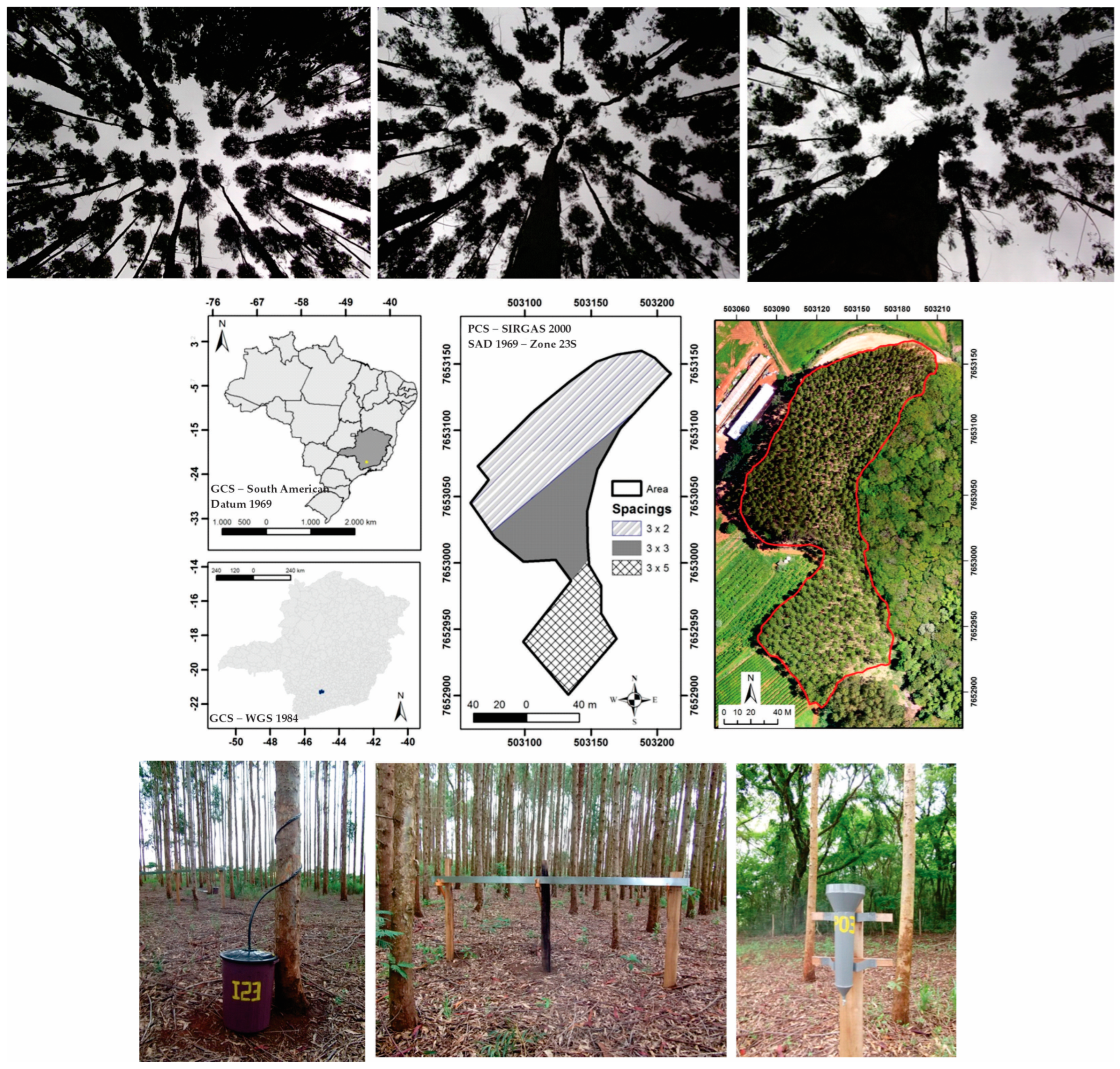
The study was carried out in an experimental area of 1.54 ha planted with eucalyptus in southern Minas Gerais state, southeastern Brazil, between the coordinates 21°19′ S and 44°58′ W (Figure 1).
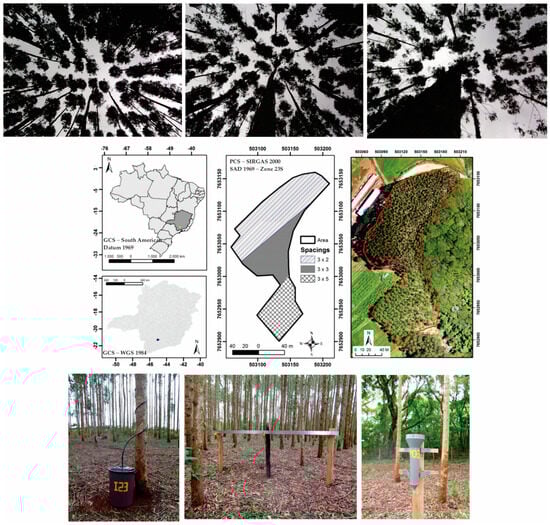
Figure 1.
Geographical location of the study area in Brazil, Lavras municipality, Minas Gerais state, instrumentation (from left to right: stemflow, gutter, and “Ville de Paris” pluviometer) used for hydrological measurements, and the different canopy openings of the eucalyptus plantation (3 m × 2 m, 3 m × 3 m, and 3 m × 5 m).
The area has two soil classes: Red–Yellow Latosol and Red Latosol, which occupy 78.6% and 21.4% of the area, respectively. The Köppen climate type of the region is Cwa, with a dry winter and a rainy summer [19].
The forest stand comprises hybrid clones of the Eucalyptus genus, primarily urophilia, and grandis genetic basis, commonly known as “Urograndis”. The trees have been strategically spaced throughout the area, with planting spacings of 3 m × 2 m (age ~ 5 years, = 15.42 cm − CV = 6.2%, = 16.46 m − CV = 8.0%, 0.77 ha and 1025 trees), 3 m × 3 m (age ~ 7 years, = 19.28 cm − CV = 6.1%, = 20.88 m − CV = 6%, 0.42 ha and 398 trees), and 3 m × 5 m (age ~ 11 years, = 22.78 cm − CV = 5.2%; = 25.05 m − CV = 4.4%, 0.35 ha and 262 trees). The different spacings and their spatial location can be seen in Figure 1.
2.2. Instrumentation
A “Ville de Paris” rain gauge was installed 150 m from the experiment to monitor external (gross) precipitation (GP) in an open, grassy area and away from obstacles [21]. The monitoring period was from November 2013 to October 2015, corresponding to two hydrological years. A weather station was in operation near the forest stand, monitoring the following weather variables on an hourly scale: air temperature (°C), relative humidity (%), atmospheric pressure (mBar), wind speed (m·s−1), and sunshine (h). These datasets were processed daily to estimate the canopy’s potential evaporation (mm·day−1) using the Penman–Monteith equation [3,17,19,21]:
where E represents potential evapotranspiration (mm·day−1), Δ is the slope of the water vapor saturation pressure curve (kPa·°C−1), Rn is the radiation balance (MJ·m−2·day−1), γ* is the modified psychometric constant (kPa·°C−1), λ is the latent heat of vaporization (MJ·kg−1), U2 is the wind speed measured at a height of 2 m (m·s−1), es is the saturation pressure of water vapor (kPa), ea is the partial pressure of water vapor (kPa), and T is the air temperature (°C).
The Gash model was individually parametrized for 17 monitoring points (trees), representing the study area. Throughfall (TF) was collected in “Ville de Paris” rain gauges placed under each monitoring tree. To avoid splash-in, these gauges were placed 150 cm above the floor [3] and had an open area of 375.8 cm2. Rainfall measurements were taken between 8 a.m. and 12 p.m. with a minimum interval of two hours after the end of the event to ensure adequate canopy drainage [19].
Stemflow (SF) was measured using collectors installed in the 17 trees. These trees were chosen based on diameter class data from the 2013 census and were distributed proportionally in the three spacings. The collectors consist of a collection and storage system with a flexible polypropylene hose attached to the trunk in a spiral form and sealed with silicone to prevent leaks when collecting all the volume drained from the canopy by the stem. The hose is directed to the sealed collector, which has a capacity of 65 L (Figure 1).
2.3. Modeling the Canopy Interception (CI)—Gash Model
The Gash analytical model for sparse canopy forests was used to model the canopy interception (CI) [9]. The model incorporates a coverage factor (c) to represent the proportion of the gross precipitation (GP) intercepted by the forest canopy per unit area. The complementary factor (p = 1 − c) represents the precipitation that freely passes through the canopy. The model assumes enough time between events for the canopy and trunks to dry completely. This study assumed that a daily-scale analysis was sufficient for this model premise [3,19].
The model is divided into three phases: (i) the wetting phase, where the incident rainfall is less than the amount needed to saturate the canopy (P′g); (ii) the saturation phase, where the rainfall intensity () is greater than the canopy evaporation rate (); and (iii) the drying phase, representing the period between the end of the rain and the time when the canopy and trunk are completely dry. Our study used average rates for incident rainfall intensity and evaporation [10,19,21]. The coverage factor (c) at each monitoring tree was estimated using the equation provided by [22]:
where k represents the extinction coefficient, and LAI is the leaf area index. A value of 0.42 was adopted for the k factor (dimensionless), which was used in hybrid stands of Eucalyptus urophilla and grandis in southeastern Brazil [23]. A LICOR LAI-2000® sensor (LI-COR Environmental, Lincoln, NE, USA) was used to estimate LAI. Ten readings were taken at each monitoring site, and an average was calculated for each point.
The Gash model presents the following structure [3,15,19]:
CIn is the canopy rainfall interception generated by each rainfall event (mm), CIs is the evaporation from the stems, CIc is the evaporation from the canopy, CIw is the canopy evaporation in the wetting phase for n rainfalls that saturate the canopy (P > P′g) (mm), CIa is the evaporation from the canopy in the drying phase (mm), CIs is the evaporation from the saturated canopy until rainfall ceases, P′g is the canopy saturation point (mm), is the average evaporation (mm h−1), is the average rainfall intensity (mm h−1), n′ is the number of rainfall events that saturate the stems (>P″g = St/Pt), St is the stem storage capacity (mm), Pt is part of P converted into SF (mm), P″g is the precipitation needed to saturate the stems, and Sc (=S/c) is the canopy storage capacity (mm). P′g can be calculated as:
To validate the Gash model, the estimated interception (CIGash) was compared to the observed interception (CIobs), which was obtained from the canopy water balance:
2.4. Gash Model Model Performance Assessment
The Pbias, Nash–Sutcliffe coefficient (NSE), and Kling–Gupta coefficient (KGE) were the precision metrics used to assess the model’s accuracy in estimating CI:
where CIGash represents the rainfall interception estimated for the ith day by the revised Gash model and CIObs is the observed interception for the ith day, both in mm, for each tree “k”. and are, respectively, the average value estimated by the Gash model and observed based on the canopy water balance. These metrics were applied twofold: (i) event-based and (ii) accumulated-based approaches. The ability of the Gash model is assessed considering each rainfall event individually (event-based), whereas (ii) accumulates the canopy interception over time (the most frequent approach). Additionally, we applied NSE and Pbias to the trees individually (only the trees used to calibrate the model). The evaluation of these metrics in hydrological models is [24] “Satisfactory” (NSE: 0.50–0.60, Pbias: 10%–15%, KGE: 0.40–0.70); “Good” (NSE: 0.60–0.80, Pbias: 3.0%–10.0%, KGE: 0.70–1.0); or “Very Good” (NSE: > 0.80, Pbias: ≤ 3.0%, KGE = 1).
3. Results and Discussion
3.1. Climate and Canopy Water Balance Observed during the Study Period
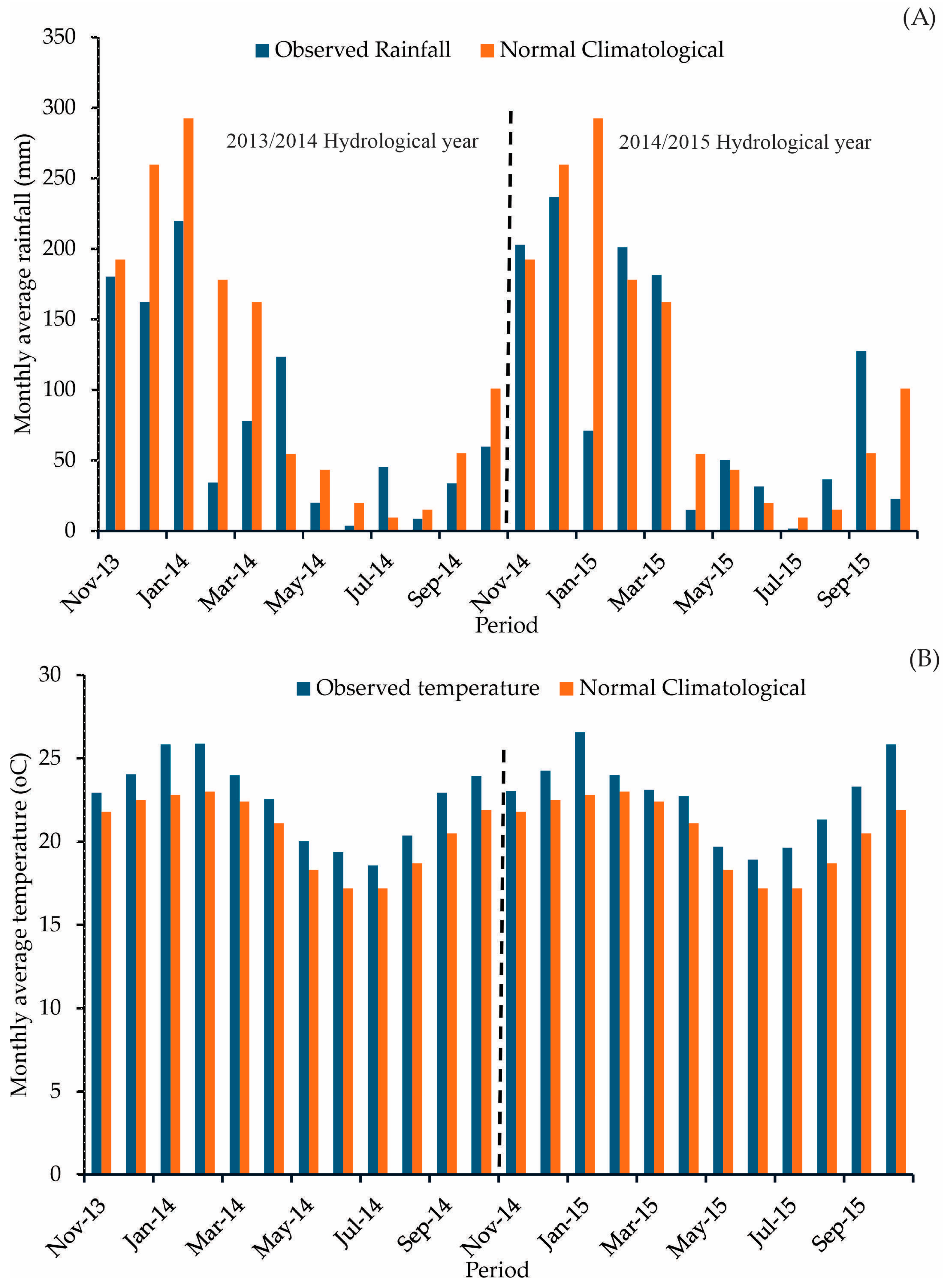
Figure 2 shows the average monthly climate data from 2013 to 2015 observed in the experimental area and the climatological normal (30-year average climatology) for the region obtained for the period of 1981–2020 [25].
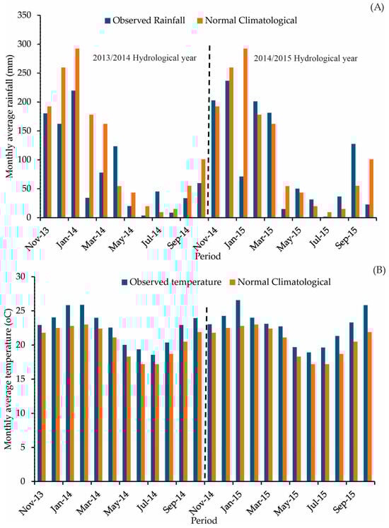
Figure 2.
Monthly observed data in the study period (2013–2015) and the last climatological normal (A) rainfall; (B) air temperature) (The dotted line separates the hydrological years).
The climate data from the study period reveal a deviation from the region’s climatological pattern. This could have major implications for forest management. The average annual air temperature was 2.0 °C higher than average between 2013 and 2015. Additionally, there was below-average rainfall during this period, with the 2013/2014 and 2014/2015 hydrological years experiencing 30% and 15% shortfall in rainfall, respectively. Particularly during the rainy season (November to March), the rainfall deficit was even more pronounced, at 37.8% and 17.7%, respectively, signaling significant droughts in the region [3].
The 2013/2014 hydrological year, one of the driest ever recorded in the region, was a rare occurrence [26]. The rainy season (November to April) accumulated only 54% of the expected rainfall. The 2014/2015 hydrological year, while showing a higher value than the previous year, also presented a negative anomaly, with 72% of the expected rainfall. These anomalies provide a unique opportunity to evaluate how forest hydrological elements respond to a climate that deviates from the region’s long-term behavior. Therefore, our results shed light on how climate change can impact hydrological eucalyptus plantation elements from a canopy water balance perspective.
Based on the average from the studied trees and hydrological years, GP, TF, CI, and SF were 1521.2 mm, 969.7 mm, 516.9 mm, and 36.6 mm. Overall, we monitored 2203 mm of GP, 1544 mm of TF (71.4% of GP), 617 mm of CI (28.5% of GP), and 41.8 mm of SF (1.9% of GP). On a daily average, GP, TF, CI, and SF were 2.96, 2.11, 0.84, and 0.057 mm d−1, respectively. Approximately 32% of the daily rainfall events in the period had values < 5 mm, and 53.1% were <10 mm. These low-intensity events and positive temperature anomalies boosted the rainfall interception in the period due to a slow saturation process and increased evaporation, likely potentialized by advection from dry surrounding areas [3,26]. TF was higher than that obtained by [27], who assessed four different eucalyptus genotypes in two hydrological years in Chile in the 3 m × 2 m planting spacing. These authors obtained TF varying from 48.6% to 68.7%, i.e., values lower than those obtained in the present study. On the other hand, they observed an SF value of 18.2% of GP without statistical difference among the genotypes. Our SF is lower (1.9%), with a high variability over time and among the trees. Our study’s forest variables DHB and H varied according to age and planting spacing. In the 3 m × 2 m spacing, the average DHB and H were 15.42 cm and 16.46 m (age ~ 5 years); in the 3 m × 3 m (age ~ 7 years), these variables were 19.28 cm and 20.88 m; and in the 3 m × 5 m (~11 years), they were 22.78 cm and 25.05 m. These differences explain the high variability of SF and TF in our experiment. In the canopy water balance study of [23] conducted in southern Brazil, TF, CI, and SF varied, respectively, from 57% to 90%, 12% to 48%, and 0.3% to 5.4% in the planting spacing of 3.0 m × 2.2 m. These values are closer to the results obtained in this study conducted in Minas Gerais state in a similar spacing. However, there are some methodological differences regarding our research. First, ref. [23] relied on gutters to measure TF, while we predominantly used Ville de Paris pluviometers for the 3 m × 2 m and 3 m × 3 m spacing and gutters for 3 m × 5 m spacing. SF was measured in nine trees per plot. At the same time, in our experimental area, we used 17 trees randomly chosen in the planting spacings, showing a methodological difference that can partially explain the difference in SF values in both studies.
Regardless of the planting spacing, the most frequent TF events were <5 mm, CI < 2.5 mm, and SF < 0.2 mm. [6] also observed similar behavior in a global metadata study for rainfall partitioning in different climates and forests, highlighting the difficulty of statistically or physically modeling these hydrological processes. Rainfall–canopy interactions rely on species diversity, forest structure and architecture, canopy openness [28], bark characteristics [29], branch configuration, canopy stratification [30], leaf wettability, morphology, and texture [29], rainfall intensity [31], wind velocity [31], external sources of energy [28], and the Leaf Area Index [6], as well as on natural and anthropogenic disturbances (e.g., logging, thinning, fire, and drought). Such interactions are even more complex for light rains that do not saturate the canopy [32]. Although models have been physically structured to simulate the canopy water balance, they struggle to represent all these processes.
Our results demonstrate how limited such approaches can be even in a planted forest, such as eucalyptus genotypes following specific planting spacing. In addition, the weather was notably different from the average climatology, i.e., negative anomalies of precipitation and positive anomalies of the temperature, which increased variability in the forest hydrological elements. Therefore, we adopted trees for the parametrization of the Gash model rather than regressions to better understand the variability of the model’s parameters in the forest. In addition, we could use the entire series of rainfall events for validation and calculate the metrics, as the study period was constrained by rainfall occurrences.
3.2. Parametrization of the Gash Model
Table 1 shows the mean values and ranges of the Gash model parameters for sparse forests obtained for a eucalyptus plantation in southeastern Brazil. Notably, average parameters were retrieved from the values obtained for each tree. We can highlight the parameter (mean rainfall intensity in the canopy), which is lower than the value calibrated by [19] (2.5 mm h−1) in an Atlantic Forest stand near the eucalyptus plantation but using datasets from 2012 observed directly over the forest canopy by a meteorological station in a 22 m tower. We can also observe that the canopy storage capacity (S) is 1.46 mm, varying from 0.94 mm to 2.11 mm. This range reflects the hydrological behavior of the trees and the intrinsic variability caused by the weather conditions and different planting spacings. The variability in the canopy parameters is highlighted even in a planted forest, following specific spacings.

Table 1.
Gash model parameters for the studied eucalyptus plantation, considering the 17 trees used in the parametrization.
The cover factor parameter (c) allows us to infer the openness of the Eucalyptus plantation canopy. [11] found a c parameter of 0.60 when studying a stand of Eucalyptus globulus in Portugal. Ref. [33] discovered a value of 0.58, close to that of this study, for Eucalyptus grandis and Urophylla hybrids. The parameter variation (Table 1) is linked to different planting spacing, mainly in 3 m × 5 m, used in the experimental area and the variability of hydrological variables obtained for this forest caused by drier hydrological years, notably in the rainy period (Figure 3).
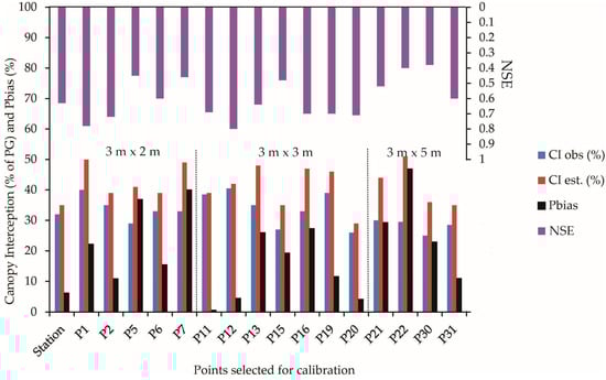
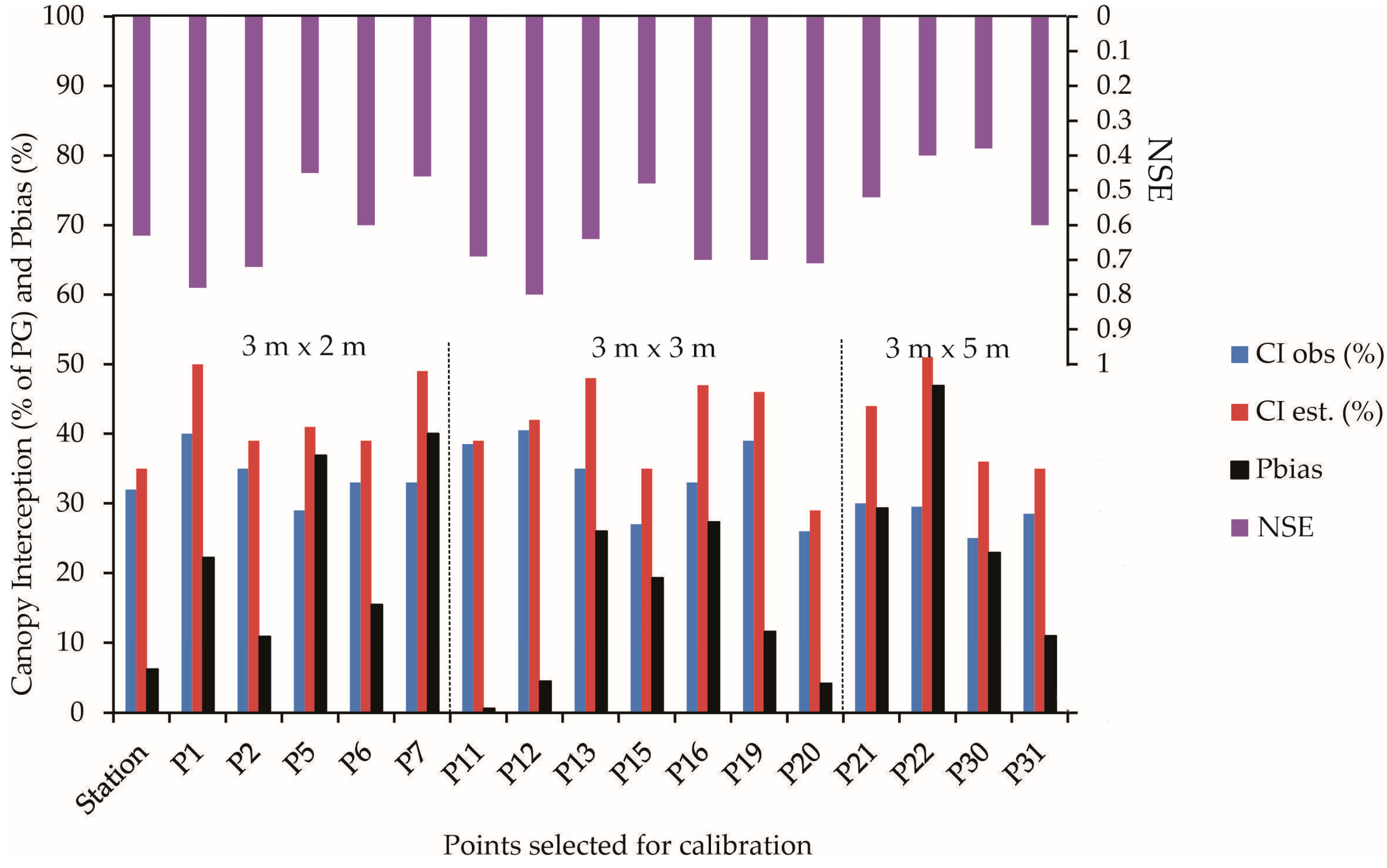
Figure 3.
Observed and estimated I (% about GP) and the statistical metrics considering the trees individually (Dotted line separates the trees under different spacings).
The free precipitation coefficient (p) is a physical parameter characterizing the model for the sparse forest version, reflecting how sparse the forest is compared to dense forests. On average, 46% of the gross precipitation passes through the canopy, contributing directly to the effective precipitation. However, like the c parameter, p also shows significant variation over the forest, influencing the model’s accuracy and increasing the trunk interception estimates. On average, the fraction of free precipitation converted into stemflow (pt) is 6%; however, we obtained up to 49%, leading to expressive variability.
Canopy storage capacity (S) is the most critical parameter in modeling rainfall interception as it influences the water that can meet the hydrological processes after interception. The average forest storage capacity, obtained by summing up canopy and trunk storage capacity, is 1.70 mm. This parameter showed a wide range between the trees, with differences of up to 75%, even for a planted forest with a uniform canopy. Compared with the Atlantic Forest, in an experimental area near the area of this study between 2012 and 2015, ref. [19] found an average value of 2.31 mm, a considerably greater value, indicating a canopy closer than the eucalyptus and a higher level of interception and evaporation.
The average evaporation rate parameter (Ē) was 0.15 mm·h−1, consistent with values found for tropical regions [17,33], ranging from 0.10 to 0.32 mm·h−1. The value estimated by [19] was slightly lower (0.104 mm h−1) due to a wet year with more rainy days, which tends to a reduced evaporation parameter estimate (both studies use the Penman–Monteith model). Ē relies on climate conditions, with greater values observed for semi-arid regions (up to ~0.94 mm·h−1; ref. [34]) and in tropical areas under drought conditions (up to 0.35 mm·h−1; ref. [3]). However, these studies used different methodologies to calculate Ē, i.e., another source of uncertainty [34]. The average gross rainfall intensity was 0.94 mm·h−1, lower than the values found in tropical regions, such as [17] (7.13 mm·h−1), ref. [20] (6.0 mm·h−1), ref. [35] (1.95 mm·h−1), and [19] (2.76 mm·h−1). This lower average intensity value occurred because this study was conducted during two considerably dry hydrological years, one of which was among the driest observed in the region in the last 100 years [26]. Consequently, the number of precipitation events was lower than the average, and such events were of low to medium intensity, reducing the average rainfall intensity and resulting in 34 events entirely intercepted due to their small volume (<1.70 mm) and very low intensity.
Except for p, and parameters, all the others decreased as the spacing between individuals increased (Table 2). The coverage factor (c) stands out, with a difference of 20.8% between the 3 m × 2 m and 3 m × 5 m spacings due to the leaf area index, while p increases in the same proportion. The smaller spacing allows a closer canopy and a higher LAI. On the other hand, wider spacing enables an opener canopy and less leaf overlap, directly affecting parameters associated with canopy architecture and the redistribution of gross precipitation. The contribution of free rainfall to throughfall increases with spacings. Moreover, the increased value of Ēc with the wider spacings reinforces the importance of considering the sparse Gash model for correctly modeling the canopy interception in planted forests.
Table 2.
Average values and respective coefficient of variation (CV, %) of the Gash model parameters calibrated according to the spacing plantings of the eucalyptus plantation.
3.3. Performance of the Modified Gash Model in the Eucalyptus Plantation
The average canopy interception estimated by the Gash model for the eucalyptus stand was 671.9 mm, representing 30.5% of the gross precipitation (GP). This value is 8.9% higher than the observed CI, which was 616.8 mm (28.0% of GP).
Figure 3 illustrates the percentage of rainfall interception estimated by the Gash model for each tree in the study. It also includes the results of the precision statistics used to assess the model’s performance for each tree and event-based approach. The Gash model consistently overestimates CI for all trees. The overestimation varies according to planting spacings, with the most accurate model fitting for the 3 m × 2 m spacing. Only one tree (P7) in this spacing showed a difference (CIGash–CIobs) that was more significant (>15%), indicating the highest Pbias. The model’s accuracy decreases for 3 m × 3 m and is more pronounced for 3 m × 5 m spacing. In the 3 m × 3 m spacing, two trees showed a difference of approximately 15%, while in the 3 m × 5 m spacing, three out of four trees showed significant differences (P22 > 20%; P21 and P30 > 15%), with P22 presenting the highest Pbias among the 17 trees.
The precision metrics reveal the “satisfactory” performance of the Gash model in estimating rainfall partitioning for eight individual trees, with the NSE > 0.50. However, with the Pbias coefficient > |15|% for nine trees, the model’s performance can be classified as “poor” for these trees, as established by hydrological models [25,36], despite the NSE > 0.5 for the trees P1, P13, and P16. These metrics indicate that the Gash model’s performance was “satisfactory” for eight individual trees, providing a good perspective for further research and application in planted forests like eucalyptus plantations. This application, particularly in the absence of sub-woods in the uniform canopy, as observed in tropical native forests, goes to confirm the model’s precision in identifying the canopy’s parameters. The estimated interception showed the most significant deviation at point P22, with an overestimate of 18.1%, while the lowest deviation was 1.2% at point P20. The main limitation for individual tree evaluation was the Pbias, constraining the model application for nine trees but being satisfactory for the other eight trees. The NSE can be considered acceptable (>0.50) for all the trees studied except for P30 (0.38), P22 (0.40), P7 (0.45), and P5 (0.44). However, Pbias indicated that the simulation might be inadequate when some trees were analyzed, like P01 (22%), P05 (36.9%), P07 (40.0%), P13 (26.0%), P15 (20%), P16 (27.3%), P21 (29.3%), P22 (46.9%), and P30 (24%). These trees had an increase in estimated interception in response to the model, and they were found in all planting spacings (Figure 3). This increase in estimated interception could be due to factors such as the tree’s size, shape, or the specific microclimate it is in, which the model may not fully account for, leading to its overestimation of interception for these trees. Since these high Pbias were observed in all spacings, the poor behavior of the Gash model was likely due to the consideration of a fixed S throughout the study period, as this model is sensitive to S [19,37,38,39]. We have observed alterations in the canopy structure during field campaigns, e.g., leaf loss, dying branches, and trees, which likely decreased canopy interception. These modifications were punctual and need further investigation, but the severe drought faced by this Eucalyptus stand may have impacted these results [28].
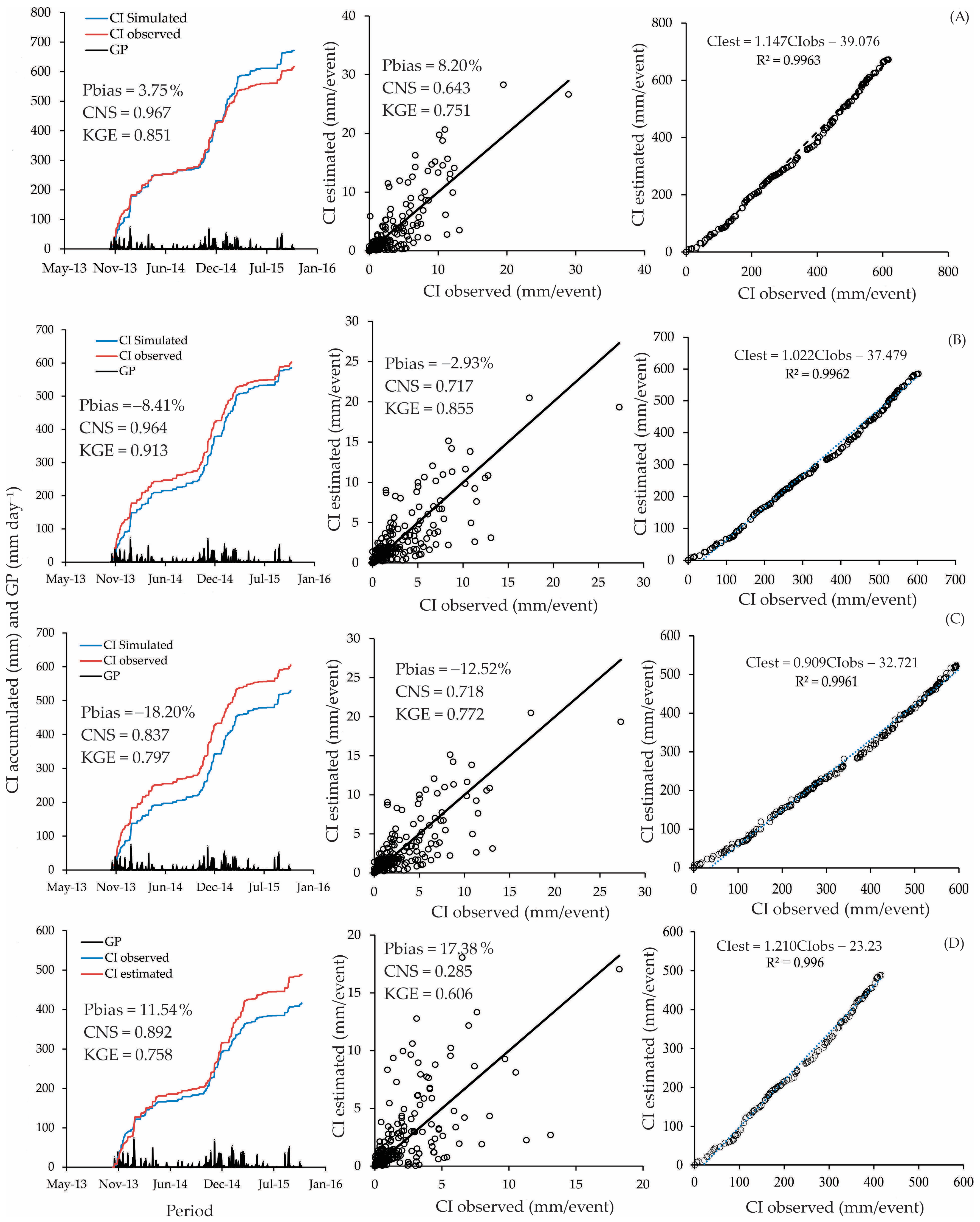
We averaged the parameters according to the respective spacing and calculated the metrics based on rainfall accumulation. The application of the Gash model to the entire area, considering the three planting spacings and the 17 trees, resulted in a “good” performance when the events were accumulated (NSE = 0.967, Pbias = 3.75%, KGE = 0.851). The same performance was also obtained for the 3 m × 2 m planting spacing (NSE = 0.964, Pbias = −8.41%, KGE = 0.913). The accumulated approach is standard but tends to inflate accuracy metrics, as variability is reduced when the data are accumulated. We observed perfect relationships between estimated and observed accumulated CI, with R2 > 0.99 for all planting spacings (Figure 4).
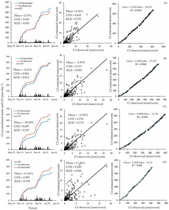
Figure 4.
Performance of the Gash model using accumulated and event-based approaches for metrics estimation ((A) the entire area; (B) 3 m × 2 m; (C) 3 m × 3 m; (D) 3 m × 5 m).
The precision metrics for accumulated events showed higher KGE values, ranging from 0.758 to 0.931. The KGE for event-based metrics varied from 0.606 to 0.855. However, the most significant reduction was observed for the NSE, which ranged from 0.837 to 0.967 for accumulated-based metrics and from 0.285 to 0.718 for event-based metrics. Despite these metrics being compatible with “good” performance for the model, the Pbias values were higher than 15%, which does not allow one to classify the Gash model performance as “good” or even “satisfactory” for 3 m × 3 m and 3 m × 5 m spacings.
The NSE and Pbias metrics indicate that the model is unsuitable for the parametrization obtained for 3 m × 5 m spacing when using event-based metrics, taking the range of these statistics established for assessing hydrological models. The poor performance in the event-based metrics sheds light on the necessity of deepening the study of canopy interception modeling, since previous studies may have inflated its ability, hindering new propositions and developments.
Using accumulated events for the metrics, [11] found an accuracy of 81.2%, 99.8%, and 80.3% for estimating CI, TF, and SF, respectively, when applying the Gash model to eucalyptus and pinus in Portugal. Ref. [16] obtained NSE values from 0.59 to 0.99 with deviations of −10.2% to 1.7% between the estimated and observed data. Ref. [33] found NSE values between 0.76 and 0.78 when estimating TF using the Rutter model for Pinus taeda sparse forests in Brazil.
Our research underscores the need for more studies on rainfall interception models for eucalyptus plantations. Most studies do not consider event-based metrics calculation, making performance comparison challenging. However, to apply the Gash model in a broader hydrological model, the simulation of the physical processes is done on an event-based basis, not an accumulated basis, i.e., in a broader water balance application, interception models need to be considered in an event-based approach. Thus, analyzing the Gash model’s performance considering event-based models is a particular approach to validating rainfall interception models that should be appraised in future studies.
4. Conclusions
This study was conducted in a planted eucalyptus plantation in southeast Brazil, considering three planting spacings: 3 m × 2 m (~5-year-old), 3 m × 3 m (~7-year-old), and 3 m × 5 m (~11-year-old). The study period encompassed the 2013/2014 and 2014/2015 hydrological years. We observed a total GP, TF, CI, and SF of 2203 mm, 1544 mm (71.4%), 617 mm (28.5%), and 41.8 mm (1.9%).
We fitted the Gash model based on 17 individual trees, generating a set of parameters for each tree. We tested the model for the entire area and the planting spacings, averaging the model parameters and calculating the precision metrics using the event and accumulated-based approaches. The Gash model overestimated CI, mainly for individual trees and event-based metrics calculation. Based on the precision metrics and the former approach, the estimated CI showed an average deviation of 18.5% regarding the observed data, NSE equal to 0.59, and Pbias of 18.2%. In this case, the Gash model showed a poor performance for nine trees and a “satisfactory” performance for the other eight trees. These metrics increased when applied to the entire area, either accumulated or event-based, and the model is classified as “good.” For the 3 m × 3 m and 3 m × 5 m planting spacings, the Pbias limited the model’s performance.
The 3 m × 5 m spacing showed more significant deviations between the observed interception loss data and that estimated by the Gash model for sparse forests compared to the other spacings for all the periods analyzed in this study. Considering the event-based approach, NSE and Pbias were 0.285 and 17.38% for this spacing, which characterizes an unsuitable model.
Based on our results for a eucalyptus plantation, we strongly recommend using the average parameters from the monitored trees and an event-based approach for precision metrics to assess the rainfall interception model’s capabilities.
Author Contributions
Conceptualization, C.R.M. and J.O.M.N.; methodology, C.R.M., J.O.M.N. and A.F.R.; software, J.O.M.N.; validation, C.R.M. and A.F.R.; formal analysis, C.R.M.; investigation, J.O.M.N.; resources, C.R.M.; data curation, C.R.M. and J.O.M.N.; writing—original draft preparation, C.R.M., J.O.M.N. and A.F.R.; editing, C.R.M. and A.F.R.; visualization, J.O.M.N.; supervision, C.R.M.; project administration, C.R.M.; funding acquisition, C.R.M. All authors have read and agreed to the published version of the manuscript.
Funding
This research received no external funding.
Data Availability Statement
The datasets of this study are available upon reasonable request.
Conflicts of Interest
The authors declare no conflicts of interest.
References
- Wu, Q.; Yang, R.; Zeng, H.; Wang, X.; Chen, G. Responses of rainfall partitioning to water conditions in Chinese forests. J. Hydrol. 2024, 637, 131410. [Google Scholar] [CrossRef]
- Vose, J.M.; Sun, G.; Ford, C.R.; Bredemier, M.; Ostsuki, K.; Zhang, Z.; Zhang, L. Forest ecohydrological research in the 21st century: What are the critical needs? Ecohydrology 2011, 4, 146–158. [Google Scholar] [CrossRef]
- Rodrigues, A.F.; Mello, C.R.; Nehren, U.; Ribeiro, J.P.C.; Mantovani, V.A.; Mello, J.M. Modeling canopy interception under drought conditions: The relevance of evaporation and extra sources of energy. J. Environ. Manag. 2021, 292, 112710. [Google Scholar] [CrossRef] [PubMed]
- Sari, V.; Paiva, E.M.C.D.; Paiva, J.B.D. Precipitação interna em floresta Atlântica: Comparação entre sistemas de monitoramento fixo e móvel. Rev. Bras. Recur. Hídricos 2015, 20, 849–861. [Google Scholar]
- Link, T.E.; Unsworth, M.; Marks, D. The dynamics of rainfall interception by a seasonal temperate rainforest. Agric. For. Meteorol. 2004, 124, 171–191. [Google Scholar] [CrossRef]
- Mello, C.R.; Guo, L.; Yuan, C.; Rodrigues, A.F.; Lima, R.R.; Terra, M.C.N.S. Deciphering global patterns of forest canopy rainfall interception (FCRI): A synthesis of geographical, forest species, and methodological influences. J. Environ. Manag. 2024, 358, 120879. [Google Scholar] [CrossRef]
- Czikowsky, M.J.; Fitzjarrald, D.R. Detecting rainfall interception in an Amazonian rain forest with eddy flux measurements. J. Hydrol. 2009, 377, 92–105. [Google Scholar] [CrossRef]
- Rutter, A.J.; Kershaw, K.A.; Robins, P.C.; Morton, A.J. A predictive model of rainfall interception forest, 1. Derivation of the model from observations in a plantation of Corsican Pine. Agric. Meteorol. 1971, 9, 367–384. [Google Scholar] [CrossRef]
- Gash, J.H.C.; Lloyd, C.R.; Lachaud, G. Estimating sparse forest rainfall interception with an analytical model. J. Hydrol. 1995, 170, 79–86. [Google Scholar] [CrossRef]
- Liu, S. A new model for the prediction of rainfall interception in forest canopies. Ecol. Model. 1997, 99, 151–159. [Google Scholar] [CrossRef]
- Valente, F.; David, J.S.; Gash, J.H.C. Modelling interception loss for two sparse eucalypt and pine forest in Central Portugal using reformulated Rutter and Gash analytical models. J. Hydrol. 1997, 190, 141–162. [Google Scholar] [CrossRef]
- Dijk, A.I.J.M.V.; Bruijnzeel, L.A. Modelling rainfall interception by vegetation of variable density using an adapted analytical model. Part 1. Model description. J. Hydrol. 2001, 247, 230–238. [Google Scholar] [CrossRef]
- Gash, J.H.C. An analytical model of rainfall interception by forests. Q. J. R. Meteorol. Soc. 1979, 105, 43–55. [Google Scholar] [CrossRef]
- Yang, J.; He, Z.; Feng, J.; Lin, P.; Du, J.; Guo, L.; Liu, Y.; Yan, J. Rainfall interception measurements and modeling in a semiarid evergreen spruce (Picea crassifolia) forest. Agric. For. Meteorol. 2023, 328, 109257. [Google Scholar] [CrossRef]
- Jackson, N.A. Measured and modelled rainfall interception loss from an agroforestry system in Kenya. Agric. For. Meteorol. 2000, 100, 323–336. [Google Scholar] [CrossRef]
- Bryant, M.L.; Bhat, S.; Jacobs, J.M. Measurements and modeling of throughfall variability for five forest communities in the southeastern US. J. Hydrol. 2005, 312, 95–108. [Google Scholar] [CrossRef]
- Cuartas, L.A.; Tomasella, J.; Nobre, A.D.; Hodnett, M.G.; Waterloo, M.J.; Múnera, J.C. Interception water-partitioning dynamics for a pristine rainforest in Central Amazonia: Marked differences between normal and dry years. Agric. For. Meteorol. 2007, 145, 69–83. [Google Scholar] [CrossRef]
- Sá, J.H.M.; Chaffe, P.L.B.; Oliveira, D.Y. Análise comparativa dos modelos de Gash e de Rutter para a estimativa da interceptação por floresta ombrófila mista. Rev. Bras. Recur. Hídricos 2015, 20, 1008–1018. [Google Scholar]
- Junqueira Junior, J.A.; Mello, C.R.; Mello, J.M.; Scolforo, H.F.; Beskow, S.; McCarter, J. Rainfall partitioning measurement and rainfall interception modelling in a tropical semi-deciduous Atlantic forest remnant. Agric. For. Meteorol. 2019, 275, 170–183. [Google Scholar] [CrossRef]
- Muzylo, A.; Llorens, P.; Valente, F.; Keizer, J.J.; Domingo, F.; Gash, J.H.C. A review of rainfall interception modelling. J. Hydrol. 2009, 370, 191–206. [Google Scholar] [CrossRef]
- Ghimire, C.P.; Bruijnzeel, L.A.; Lubczynski, M.W.; Ravelona, M.; Zwartendijk, B.W.; van Meerveld, H.J. Measurement and modeling of rainfall interception by two differently aged secondary forest in upland eastern Madagascar. J. Hydrol. 2017, 545, 212–225. [Google Scholar] [CrossRef]
- Almeida, A.Q.; Ribeiro, A.; Leite, F.P. Modelagem do balanço hídrico em microbacia cultivada com plantio comercial de Eucalyptus grandis × urophylla no leste de Minas Gerais, Brasil. Rev. Árvore 2013, 37, 547–556. [Google Scholar] [CrossRef]
- Ferreto, D.O.C.; Reichert, J.M.; Cavalcante, R.B.L.; Srinivasan, R. Rainfall partitioning in young clonal plantations Eucalyptus species in a subtropical environment, and implications for water and forest management. Int. Soil Water Conserv. Res. 2021, 9, 474–484. [Google Scholar] [CrossRef]
- Moriasi, D.; Gitau, M.; Pai, N.; Daggupati, P. Hydrologic and Water Quality Models: Performance Measures and Evaluation Criteria. Trans. ASABE 2015, 58, 1763–1785. [Google Scholar]
- Instituto Nacional de Meteorologia (INMET). Normais Climatológicas do Brasil: 1991–2020; INMET: Brasília, Brazil, 2022. [Google Scholar]
- Silva, V.O.; Mello, C.R. Meteorological droughts in part of southeastern Brazil: Understanding the last 100 years. An. Acad. Bras. Cienc. 2021, 93 (Suppl. S4), e20201130. [Google Scholar] [CrossRef]
- Valverde, J.C.; Rubilar, R.; Barrientos, G.; Medina, A.; Pincheira, M.; Emhart, V.; Zapata, A.; Bozo, D.; Espinoza, Y.; Campoe, O.C. Differences in rainfall interception among Eucalyptus genotypes. Trees 2023, 37, 1189–1200. [Google Scholar] [CrossRef]
- Rodrigues, A.F.; Terra, M.C.; Mantovani, V.A.; Cordeiro, N.G.; Ribeiro, J.P.; Guo, L.; Nehren, U.; Mello, J.M.; Mello, C.R. Throughfall spatial variability in a neotropical forest: Have we correctly accounted for time stability? J. Hydrol. 2022, 608, 127632. [Google Scholar] [CrossRef]
- Tonello, K.C.; van Stan II, J.T.; Rosa, A.G.; Balbinot, L.; Pereira, L.C.; Bramorski, J. Stemflow variability across tree stem and canopy traits in the Brazilian Cerrado. Agric. For. Meteorol. 2021, 308–309, 108551. [Google Scholar] [CrossRef]
- Lian, X.; Zhao, W.; Gentine, P. Recent global decline in rainfall interception loss due to altered rainfall regimes. Nat. Commun. 2022, 13, 7642. [Google Scholar] [CrossRef]
- Nanko, K.; Onda, Y.; Ito, A.; Moriwaki, H. Spatial variability of throughfall under a single tree: Experimental study of rainfall amount, raindrops, and kinetic energy. Agric. For. Meteorol. 2011, 151, 1173–1182. [Google Scholar] [CrossRef]
- Kochendorfer, J.; Paw U, K.T. Field estimates of scalar advection across a canopy edge. Agric. For. Meteorol. 2011, 151, 585–594. [Google Scholar] [CrossRef]
- Steidle Neto, A.J.; Ribeiro, A.; Lopes, D.C.; Sacramento Neto, O.B.; Souza, W.G.; Santana, M.O. Simulation of rainfall interception of canopy and litter in Eucalyptus plantation in tropical climate. For. Sci. 2012, 58, 54–60. [Google Scholar] [CrossRef]
- Navar, J. Modeling rainfall interception components of forests: Extending drip equations. Agric. For. Meteorol. 2019, 279, 107704. [Google Scholar]
- Vieira, C.P.; Palmier, L.R. Medida e modelagem da interceptação da chuva em uma área florestada na região metropolitana de Belo Horizonte, Minas Gerais. Rev. Bras. Recur. Hídricos 2006, 11, 101–112. [Google Scholar] [CrossRef]
- Van Liew, M.W.; Veith, T.L.; Bosch, D.D.; Arnold, J.G. Suitability of SWAT for the conservation effects assessment project: A comparison on USDA-ARS watersheds. J. Hydrol. Res. 2007, 12, 173–189. [Google Scholar]
- Wallace, J.; McJannet, D. On interception modeling of a lowland coastal rainforest in northern Queensland, Australia. J. Hydrol. 2006, 329, 477–488. [Google Scholar] [CrossRef]
- Steidle Neto, A.J.; Lopes, D.C.; Silva, T.G.F.; Souza, L.S.B. Evaluation of evaporation methods for modelling rainfall interception in a dry tropical forest. Theor. Appl. Climatol. 2024, 155, 7721–7736. [Google Scholar] [CrossRef]
- Grunicke, S.; Queck, R.; Bernhofer, C. Long-term investigation of forest canopy rainfall interception for a spruce stand. Agric. For. Meteorol. 2020, 292–293, 108125. [Google Scholar] [CrossRef]
Disclaimer/Publisher’s Note: The statements, opinions and data contained in all publications are solely those of the individual author(s) and contributor(s) and not of MDPI and/or the editor(s). MDPI and/or the editor(s) disclaim responsibility for any injury to people or property resulting from any ideas, methods, instructions or products referred to in the content. |
© 2024 by the authors. Licensee MDPI, Basel, Switzerland. This article is an open access article distributed under the terms and conditions of the Creative Commons Attribution (CC BY) license (https://creativecommons.org/licenses/by/4.0/).