A Copula Approach for Predicting Tree Sap Flow Based on Vapor Pressure Deficit

Abstract

While using sap-flow sensor measurements is a well-established technique for quantifying leaf water transpiration in tree species, installing and maintaining a large number of sensors and data loggers in large-scale plantations to obtain accurate measurements is both costly and time-consuming. We developed a copula-based approach to predict sap flows based on readily available vapor pressure deficits (VPDs) and found that the Normal copula was the best among five commonly used copulas. The Normal-copula approach was validated using our field-measured eastern cottonwood (Populus deltoides (Bartr. ex Marsh.)) sap flow data, yielding solid statistical measures, including Mann–Kendall’s τ = 0.59, R² = 0.81, and p-value < 0.01. The approach was applied to predict sap flows of eastern cottonwood during the growing period from 1 March to 31 October 2015 as well as the 5-year growing period from 2019 to 2023. It successfully replicated the characteristic diurnal sap flow pattern, with rates increasing during the day and decreasing at night, as well as the typical seasonal pattern, with rates rising from winter to summer and decreasing from summer to next winter. Our study suggests that the copula-based approach is a reliable tool for estimating sap flows based on VPD data.

1. Introduction

Heat-based sap flow measurement is a non-destructive method used to quantify the transpiration of tree species [1], while the transpiration of trees is a critical component for better-estimating forest evapotranspiration (ET) [2]. In general, forest ET is water transpiration from tree leaves plus water evaporation from bare soil, tree canopy, and open waterbodies in forest watersheds. It has been reported that forest ET contributes more than any other ecosystem to global ET, accounting for 44% of total ET [3]. Forest watersheds have long been recognized for conserving rainwater, mitigating surface water runoff, and generating clean water [4], while tree ET means a large amount of water is lost from forest watersheds, and it is a crucial surficial process for estimating hydrologic cycles and water resource availability [5,6]. Although sap flow measurement is a well-established technique used to measure tree transpiration with the advantage of continuously monitoring without modifying the ambient environment [2], this technique is costly and time-consuming because it involves the installation and maintenance of large numbers of sensors, dataloggers, and field crews in large-scale plantations for accurate measurements. Therefore, a need exists to develop practical and reliable methods for estimating tree water use in forest watersheds.

This issue may be tackled with an understanding that correlations exist between sap flow and some surficial environmental factors such as photosynthetically active radiation, air temperature, relative humidity, vapor pressure deficit (VPD), and solar radiation [7,8,9]. Nadezhdina et al. [8] measured sap flow in apple trees (Malus domestica Borkh.) and reported that the diurnal pattern of sap flow is somewhat correlated to environmental factors such as leaf water potential, air temperature, relative humidity, and solar radiation. Liu et al. [7] reported that sap flows of sawtooth oak (Quercus acutissima Carruth) and China-fir (Cunninghamia lanceolate (LAMB) Hook.) are, to a certain degree, correlated to photosynthetically active radiation, air temperature, relative humidity, VPD, precipitation, and soil water content. While the above and many other studies provide useful insights into the correlations between sap flow and surficial environmental factors, most of the correlations have a low coefficient of determination (R²). It appears that the diurnal pattern of sap flow is not strongly associated with that of environmental factors. Therefore, it is impractical to simply predict sap flux based on those environmental factors.

To circumvent this obstacle, Ouyang et al. [10] developed a STELLA (Structural Thinking and Experiential Learning Laboratory with Animation)-based model to predict the sap flow of eastern cottonwood (Populus deltoides (Bartr. ex Marsh.)) in Mississippi, USA, using VPD with adjustments. The VPD is selected in their study partially because VPD data are easy to obtain from local weather stations, and the correlation of sap flow to VPD is somewhat more substantial than other environmental factors [10]. After calibration and validation, the STELLA model was able to predict the diurnal and annual patterns of sap flow: it increases during the day and decreases at night, increases from winter to summer, and then falls from summer to next winter. The model provides a new means to predict sap flow using the readily available VPD. One primary assumption in applying this model is that the diurnal peaks of VPD and sap flow do not arrive at the same periods, and thus, the VPD peak times need to be adjusted to match those of sap flow. These adjustments vary with tree species, site conditions, and geographical locations. The major limitations of the STELLA-based model were that soil water availability is not a limiting factor for sap flux and the exceedingly high sap flux peaks were not easy to predict. Additionally, STELLA is a commercial software package (https://www.iseesystems.com/store/products/stella-architect.aspx, accessed on 10 April 2024) and may involve a moderate to steep learning curve for users. These make the applications of the STELLA-based model somewhat difficult.

Chen et al. [11] developed a statistical method to calculate sap flow using heat–response curves. While this is a viable approach, field experimental data for heat pulse are required. Recently, Li et al. [12] developed an integrated network model by combining CNN (convolutional neural network)-GRU (gated recurrent unit)-BiLSTM (bidirectional long-short-term memory) networks to predict sap flow. However, this network model would require a large amount of experimental data. To overcome these limitations, a better approach with easily obtained and/or readily available data is very necessary. To this end, a copula method is employed in this study to predict sap flow based on VPD.

Copula analysis is a multivariate statistical approach used to identify the relationships among random variables that are otherwise difficult (if not impossible) to determine by traditional methods. As an example, Ouyang [13] has successfully applied the couple method to predict stream discharge using precipitation data, which is not possible by using traditional methods. The copula method was first developed by Sklar [14] and has been widely used for multidisciplinary applications, including actuarial science, finance analysis, hydrological modeling, and water resources management [15,16,17,18,19]. In recent years, some efforts have been made to apply copula regressions to predict one variable using other variables [10,20,21]. The advantage of copula regression is that there is no restriction on probability distribution as compared to the ordinary least squares and generalized linear regression methods [22]. Masarotto and Varin [21] applied a Gaussian copula regression model to fit malaria data with an excellent linear correlation, while Cote et al. [20] ranked property and casualty insurance using copula regression. These copula-based regression studies provide beneficial insights into developing correlations among random variables. However, few efforts have been devoted to establishing the correlations among hydrological variables using copula-based regression.

This study aimed to estimate hourly tree sap flow based on hourly VPD using the copula method. Our specific objectives were to (1) select the best copula function for predicting sap flow based on VPD in the R-Statistics platform; (2) validate the predicted sap flow from the selected copula with our field-measured data; and (3) develop a copula-based regression equation and apply it to predict the eastern cottonwood sap flow when the measured data are not available.

2. Materials and Methods

2.1. Data Acquisition

The sap flow and VPD data were obtained at the eastern cottonwood biomass production plantation (Figure 1) near Hollandale, Washington County, Mississippi, USA [9]. The plantation was originally established in 2012 to study eastern cottonwood biomass production with a planting density of 1 m × 1 m and a plot area of 1.01 hectares. In this study, we installed 2 cm long laboratory-made heat-dissipation-type sensors on 18 eastern cottonwood trees in the plantation to collect sap flow from September 2016 to September 2018. One sensor pair consists of a reference sensor and a heated sensor, each containing thermocouples within hypodermic needles. The sensors for each pair were mounted about 10 cm apart vertically and then covered with insulated aluminum shielding to prevent solar radiation from impacting readings. All sensors were connected to a CR1000 datalogger and an AM 16/32/B multiplexer (Campbell Scientific Inc., Logan, UT, USA), and the instrumentation was powered by rechargeable marine deep-cycle batteries connected to a solar panel. Measured sap flow data at a 30 min collection interval were transmitted to an office computer through a wireless carrier (Verizon Inc., New York, NY, USA). Details on the sap flow measurement and data acquisition can be found in Ouyang et al. [10].

The time-series air temperature and relative humidity data (used to calculate VPD) at the same collection interval were downloaded from the on-site weather station. Missing data from the on-site station were filled with data from the nearest weather station. The time-series hourly VPD data were then calculated as [23]:

$$D_{vp}=\left[1-\left(\frac{RH}{100}\right)\right]\times 610.7\times {10}^{\frac{7.5T_{air}}{237.3+T_{air}}}$$

(1)

where D_vp is the VPD (Pa), RH is the relative humidity (%), and T_air is the air temperature (°C).

Figure 2a shows a poor correlation (R² = 0.2631) between the measured sap flow and the calculated VPD, while Figure 2b reveals that the peaks of the daily sap flow came about 4 h earlier than those of the VPD. It is apparent that we cannot use the equation shown in Figure 2a to predict sap flow based on VPD. Therefore, the copula method was employed in this study.

2.2. Copula Analysis

Several methods are used to develop copula functions, but the methods of inversion, generation, and extreme value are the most used ones [24]. Copulas built with the inversion method are elliptical, copulas derived with the generation functions are Archimedean copulas, and copulas represent the dependence structure between extreme values (or exceptional events are extreme-value copulas) [24]. Copulas derived by these methods are determined by a small number of parameters that are not flexible, especially in high dimensions. Vine copulas circumvent this obstacle and are highly flexible and numerical applicable copula classes [25,26]. A wide variety of copula families are available within the Vine copulas for selecting the dependence structure, making selection of appropriate copulas somewhat difficult. In this study, we applied the Vine copulas package in the R-Statistics platform to select the best copula out of the five commonly used bivariate copulas, namely the BB8 (Joe-Frank), Clayton, Frank, Gumbel, and Normal copulas, for fitting our sap flow and VPD data. The following six steps were employed to perform the copula analysis [10,13]:

i.

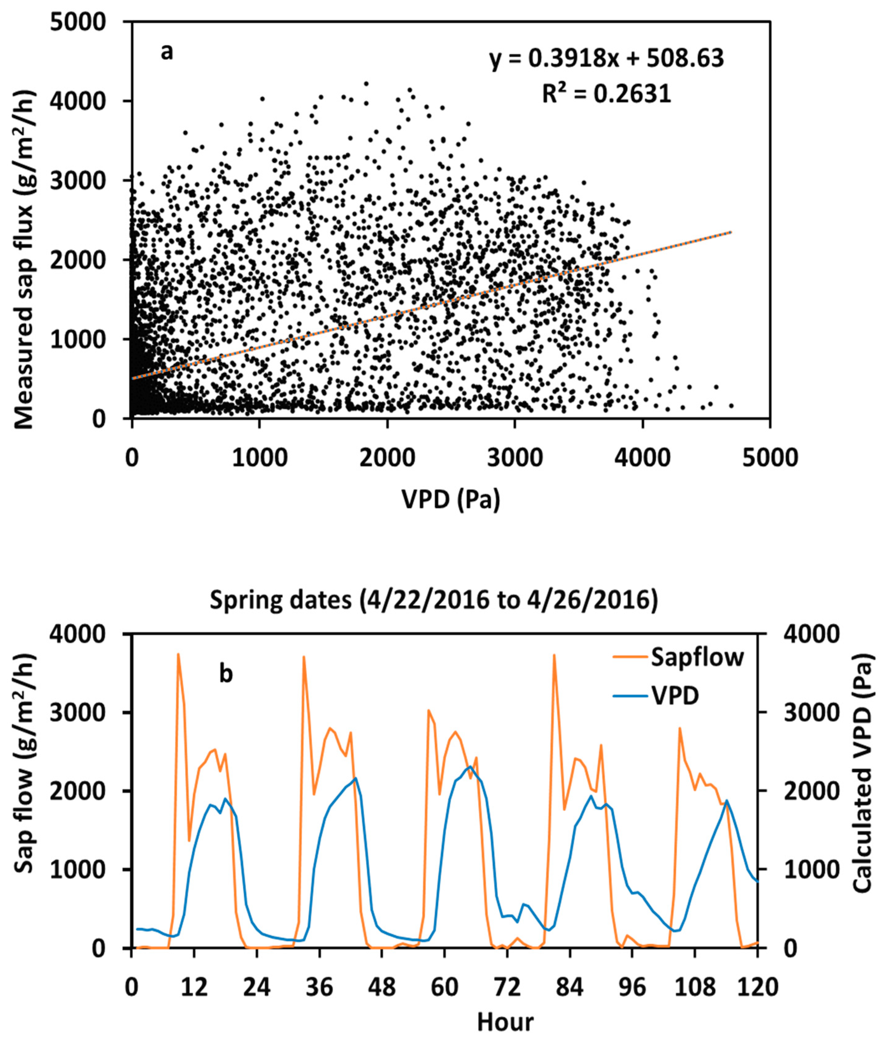
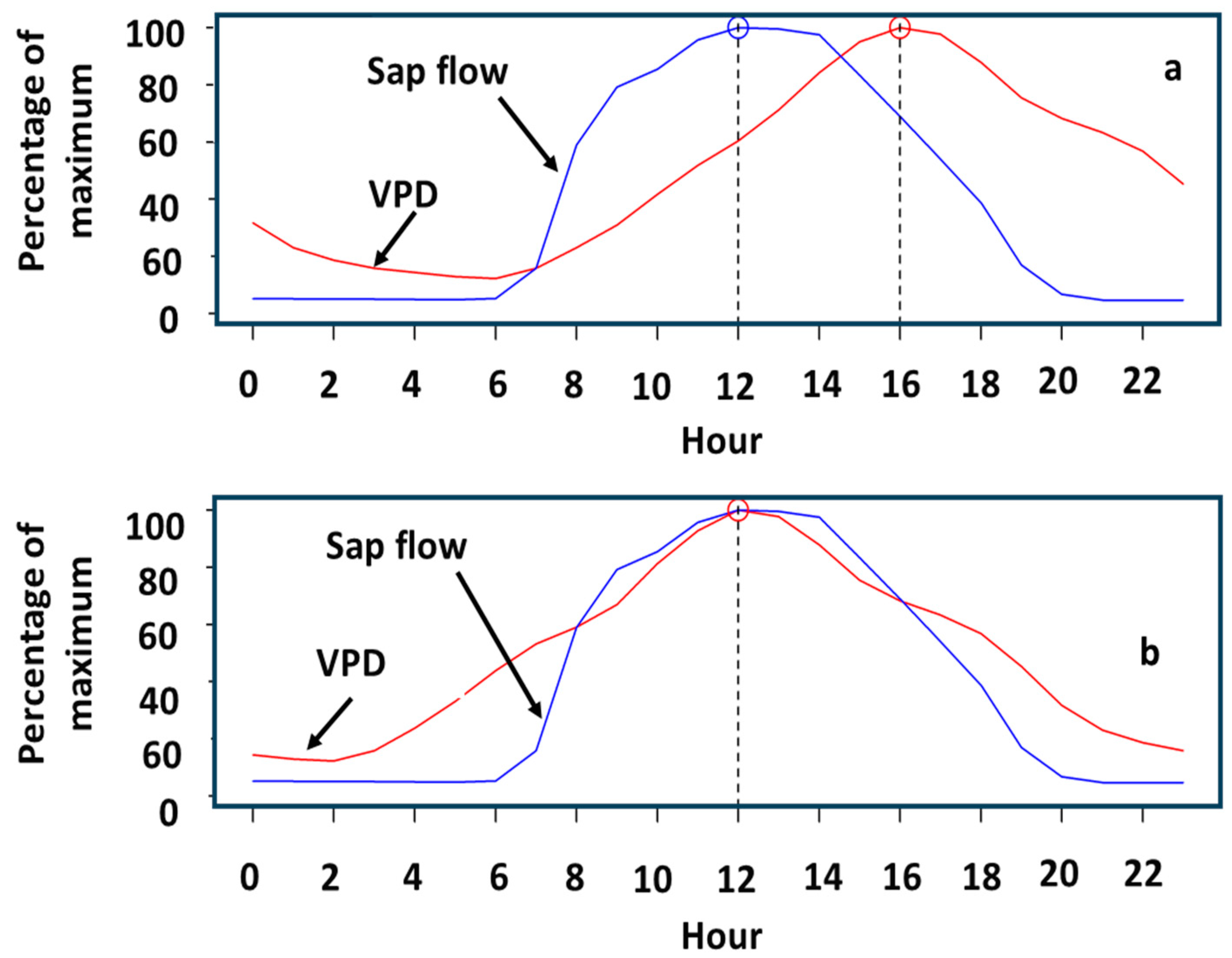
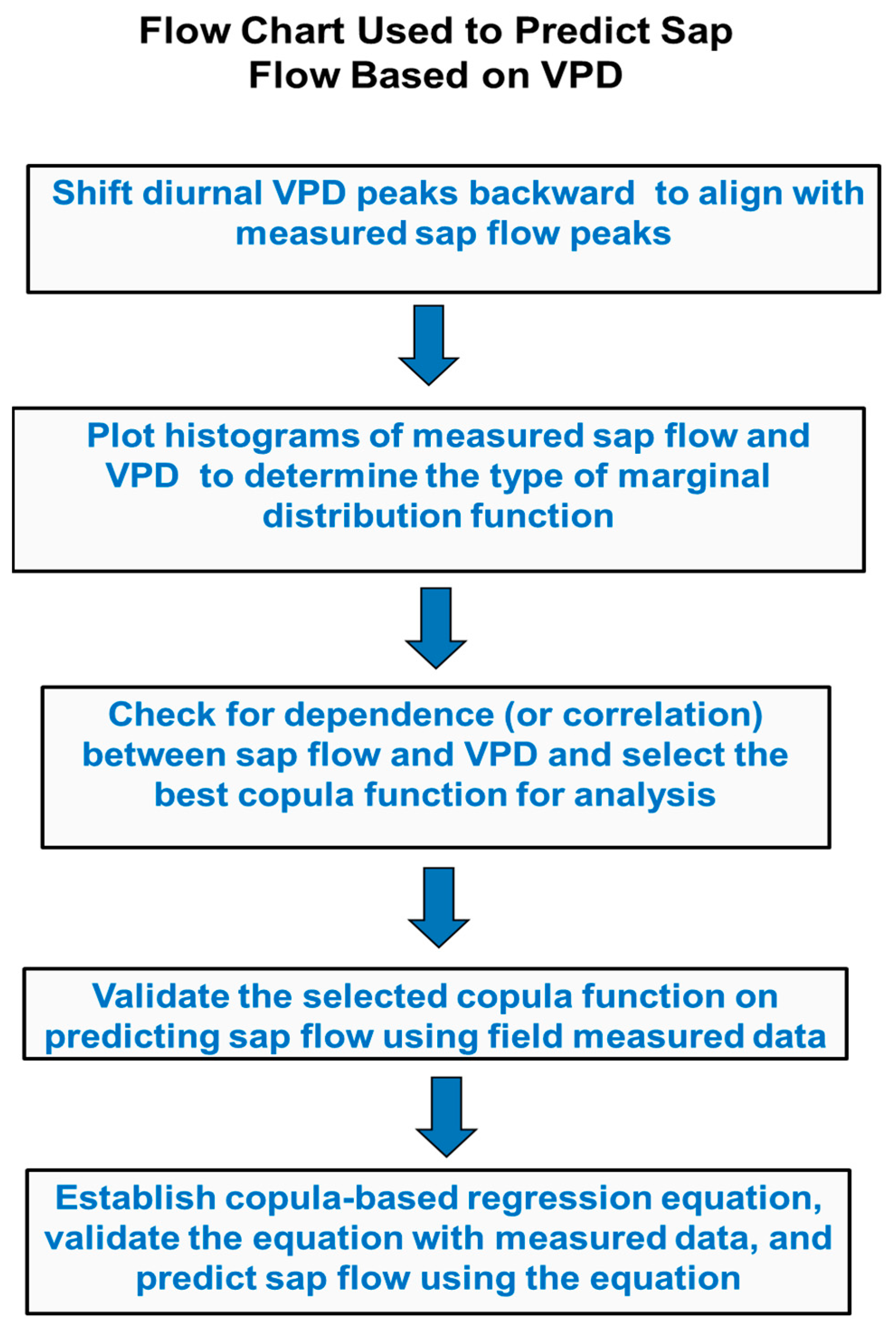
VPD data adjustment. Figure 3a shows the percentages of maximum diurnal peak values for the measured hourly sap flow and VPD. About 95% of the diurnal sap flow peaks occurred at 12 h, while about 95% of the diurnal VPD peaks took place at 16 h, indicating a 4 h lag with 95% maximum values in the sap flow and VPD data. To accurately predict hourly sap flows based on hourly VPDs, the VPDs need to be adjusted by shifting 4 h backward to align with the diurnal peaks of the sap flow (Figure 3b). This shift will obtain a better correlation between sap flow and VPD when randomly generating the correlation in copula analysis.

ii.

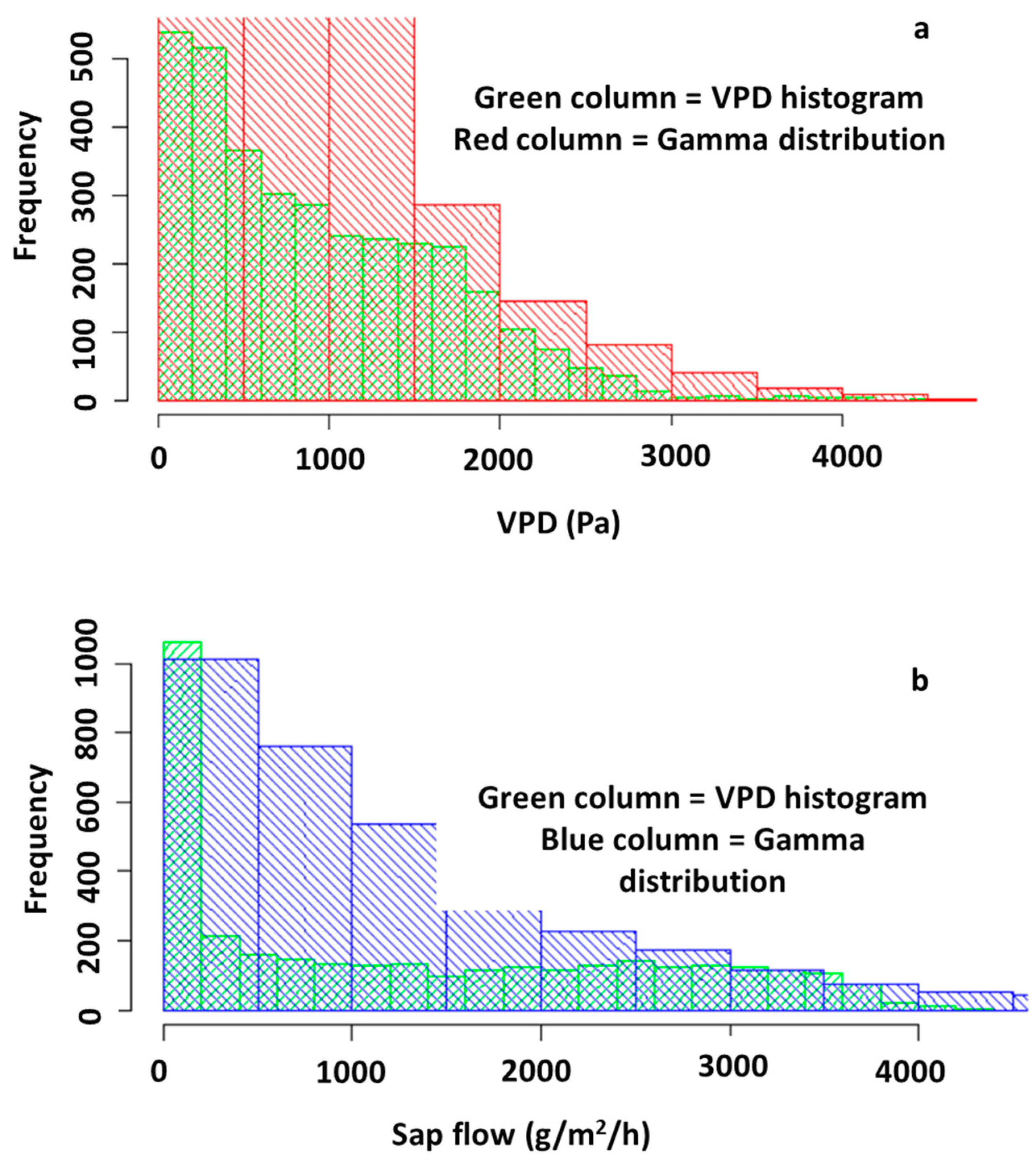
Histogram plot. A histogram plot showed a Gamma distribution of the sap flows and VPDs (Figure 4). Thus, the Gamma type of distribution was used as a marginal distribution function when building the bivariate distribution for the five copulas. In statistical analysis, the probability distribution of all its random variables is defined as a joint distribution, whereas the probability distribution of one random variable is called a marginal distribution. The marginal distribution functions play a vital role in determining dependence among random variables. Two random variables are dependent (or correlated) if and only if their joint distribution function is not equal to the product of their marginal distribution functions (https://www.statlect.com/glossary/marginal-distribution-function, accessed 10 April 2024).

iii.

Dependence of sap flow on VPD. In a copula analysis, the correlation (or dependence) of two or more variables is normally measured (or estimated) by Mann–Kendall’s tau (τ) and Spearman’s rho methods. In this study, Mann–Kendall’s τ value was used to measure the correlation (or dependence) between the sap flow and the VPD. The τ value ranges from −1 to 1. If τ = 0, no relationship exists, and if τ = 1 (or −1), a perfect relationship exists (with positive τ for an increasing trend and negative τ for a decreasing trend). The best copula function (with the highest τ value) was selected for further analysis.

iv.

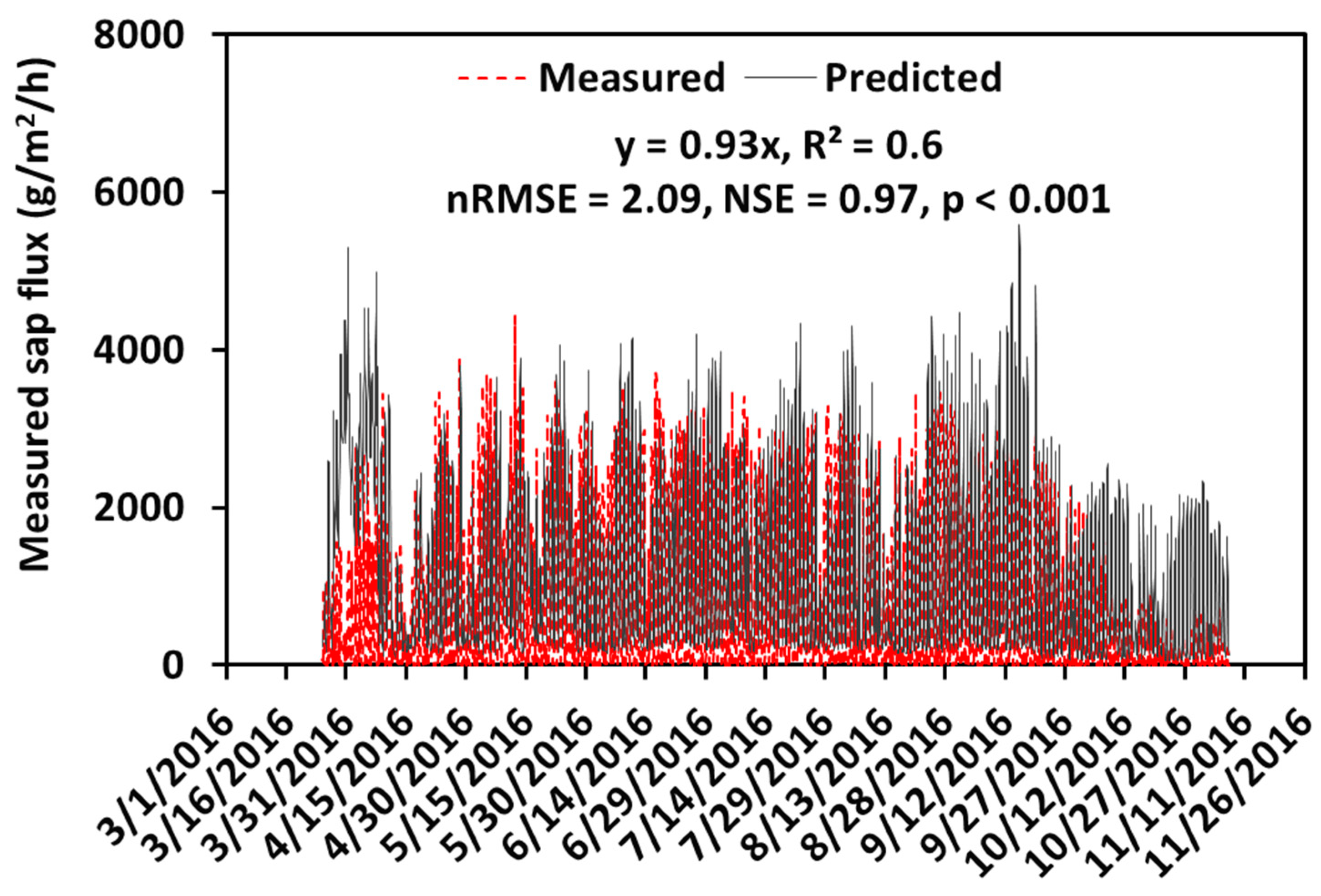
Validation of the selected copula. The selected copula function was used to predict sap flows based on VPDs. The predicted sap flows were then compared with our field measurements. The goodness-of-validation was estimated with Mann–Kendall’s τ at p < 0.01.

v.

Randomly generate sap flow and VPD data. Once the selected copula was validated, it was used to randomly generate sap flow and VPD data.

vi.

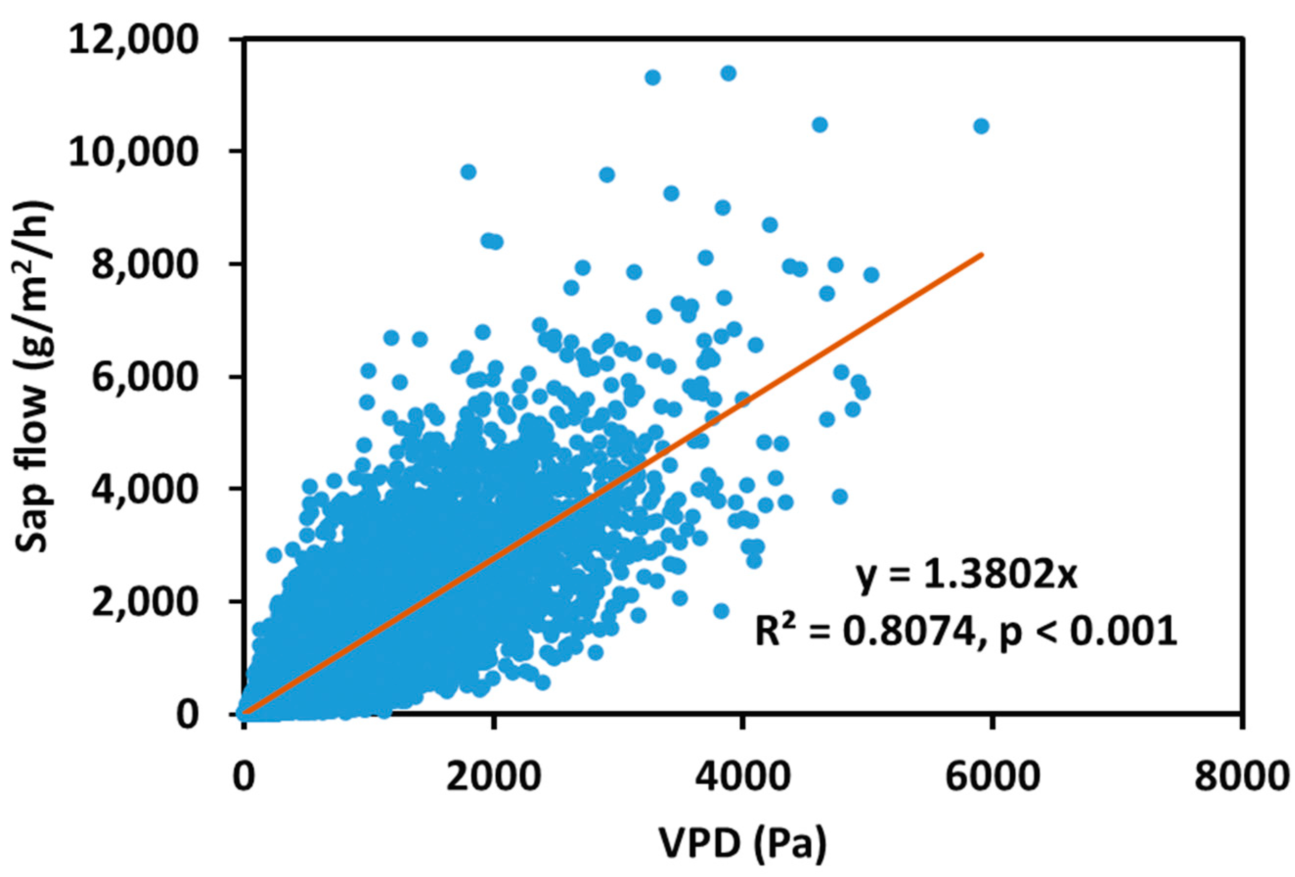
Establish a copula-based regression equation. The randomly generated sap flow and VPD data (Step 5) were used to establish a copula-based regression equation in an Excel spreadsheet. This equation was applied to predict sap flows when the VPDs were given. It should be noted that the sap flows predicted by the copula-based regression equation based on VPDs do not include the time-series component. In the real world, however, sap flow varies with times in hourly, daily, monthly, and annual manners. In other words, the sap flows predicted by the copula-based regression equation cannot be directly used because they do not tell when the sap flows occurred. Therefore, the time-series component must be included in the copula analysis. Fortunately, VPD data are always associated with time series and therefore the sap flows predicted by the copula-based regression equation based on VPDs are time-series data.

Steps ii to v were implemented using an R script (R 4.3.0) written in this study. This script is available to readers upon request. The flow chart associated with the above six steps is shown in Figure 5 for readers’ convenience.

3. Results

3.1. Copula Selection and Validation

A comparison of the Mann–Kendall’s τ and p values among the five copulas (

Table 1. Comparison of the Mann–Kendall’s τ and p values among the five copulas used to predict sap flows based on VPDs.

Copula Function	τ	p-Value
BB8	0.33	0.01
Clayton Copula	0.21	0.01
Frank Copula	0.16	0.01
Gumbel Copula	0.04	0.01
Normal Copula	0.59	0.01

) reveals that the Normal copula was the best one in predicting sap flows based on VPD data because of its highest τ value (0.59). The p-value is a statistical measure of a trend; if p ≤ 0.05, there is a monotonic trend [27].

The Normal (or Gaussian) copula belongs to the elliptical copulas family and is derived from the multivariate Gaussian or Normal distribution [28] as:

$$C_{Normal}(u_1, \dots ,u_n)={\Phi }_n[{\varphi }^{-1}\left(u_1\right),\dots ,{\varphi }^{-1}\left(u_n\right)]$$

(2)

where Φ is the cumulative distribution function (cdf) of a multivariate normal distribution with zero mean and covariance matrix, and Φ is the cdf of the standard normal distribution at θ (0, 1). The Normal copula is popular as it allows for modeling dependence in arbitrarily high dimensions with only one parameter governing the strength of dependence. The τ value for the Normal copula is calculated as:

$$\tau =\frac{2}{\pi }arcsin\theta$$

(3)

The goodness-of-fit of the Normal copula was validated by comparing the copula predicted and measured sap flows and VPDs (Figure 6). The measured hourly sap flow data were the averaged sap flow from 18 trees in the plantation from 2017 to 2018, whereas the calculated VPD data were obtained using the measured air temperature and relative humidity during the same period and Equation (1). With τ = 0.59 and p < 0.01, we concluded that the predicted sap flows matched the estimated sap flows reasonably well.

Based on the sap flow and VPD data randomly generated from the Normal copula, the following copula-based regression equation was obtained (Figure 7):

$$Y_{sap}=1.38\times D_{VPD} R^2=0.81, p<0.001$$

(4)

where Y_sap is the predicted sap flow (g/m²/h) and D_VPD is the VPD (Pa). When the time-series VPD data are available, the time-series sap flows can be predicted using Equation (4). It should be kept in mind that the sap flow predicted using Equation (4) is the average value of a tree from the plantation. For the whole plantation, the overall sap flow can be summed up if the tree planting density of a plantation is known.

While we cannot use the equation shown in Figure 2a to predict sap flow based on VPD because the sap flow had a very poor correlation (R² = 0.26) with the VPD, we can apply Equation (4) to achieve the goal because these two variables had a very good linear correlation (R² = 0.81) after copula analysis (or transformation). The results prove that a good correlation between sap flow and VPD can be established with copula transformation, which is otherwise very difficult to accomplish using traditional methods.

To develop confidence in applying the copula-based regression in Equation (4), we further validated this equation with another set of measured sap flow and VPD data during the period from 1 March to 31 October 2016 (Figure 8). With reasonable R², low normalized root-mean-square error (nRMSE), high Nash–Sutcliff efficiency (NSE), and low p-value, we concluded that the copula-based regression equation (Equation (4)) is adequate for predicting sap flows based on VPDs.

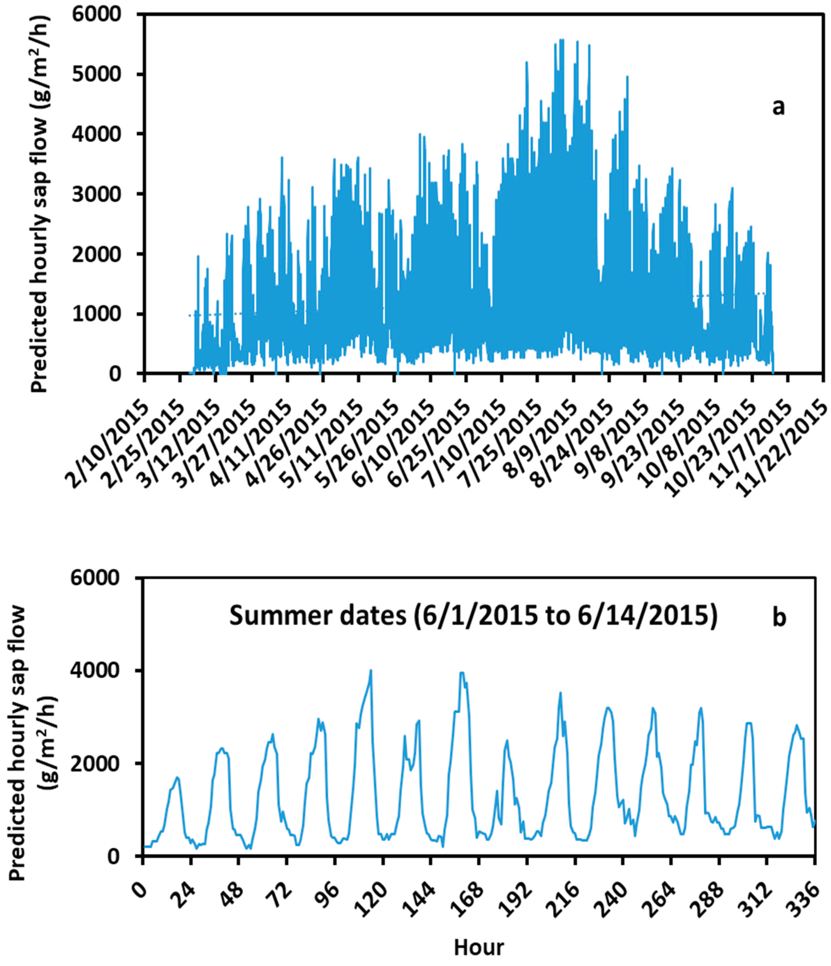
3.2. Growing Season Sap Flow Prediction

Predictions of average hourly tree sap flow in a 5-year-old eastern cottonwood plantation over a growing season from 1 March to 31 October 2015 are given in Figure 9a. The VPD data used for the predictions were calculated with Equation (1) using air temperature and relative humidity data obtained from the on-site weather station. It should be noted that the growing season of eastern cottonwood was used because a very low sap flow of eastern cottonwoods occurred during winter. As stated in the previous section, sap flow predicted with Equation (4) is the average value of a tree in the plantation.

The predicted average hourly sap flow varied from time to time over the growing season, with a maximum of 5442 g/m²/h occurring in August (Figure 9a) due to the high air temperature. The predicted average sap flow was 1311 g/m²/h during the growing season, which was comparable to our measured average sap flow of 1307 g/m²/h for the same growing season and tree species. The results indicated that the Normal copula-predicted sap flows were well within the range of the measured ones.

The monthly variation of sap flow during the growing season can be deduced from Figure 9a. The hourly sap flow increased from March, attained its maximum in August, and decreased from August to October. On average, the monthly amount of sap flow followed the order: August (1273 kg/m²) > July (1132 kg/m²) > June (985 kg/m²) > May (925 kg/m²) > September (802 kg/m²) > April (691 kg/m²) > October (608 kg/m²) > March (431 kg/m²). This pattern of monthly sap flow corresponded well to that of the monthly air temperature in Mississippi. The higher the air temperature, the larger the leaf sap flow that occurred. Similar results were obtained by Vose et al. [29]. These authors quantified the tree and stand-level transpiration of eastern cottonwoods in central Texas and reported that the highest sap flow of the eastern cottonwoods occurred during early summer.

The diurnal pattern of the predicted sap flows over a 2-week period in summer from 1 June to 14 June 2015 is shown in Figure 9b. The results showed that the sap flow increased in the early morning, reached the maximum in the late afternoon, and decreased at night. This diurnal pattern was comparable to that reported by Ouyang et al. [10], who performed a field experiment to measure eastern cottonwood sap flow at the same study site using sensors. Figure 9b further reveals that the sap flow peaks varied from day to day over the 2-week period. For example, the sap flow peak was 1710 g/m²/h at 17 h (1 June) but was 4000 g/m²/h at 114 h (5 June). The latter was about 2.3 times greater than the former. This occurred due to the variations of weather variables such as air temperature and precipitation.

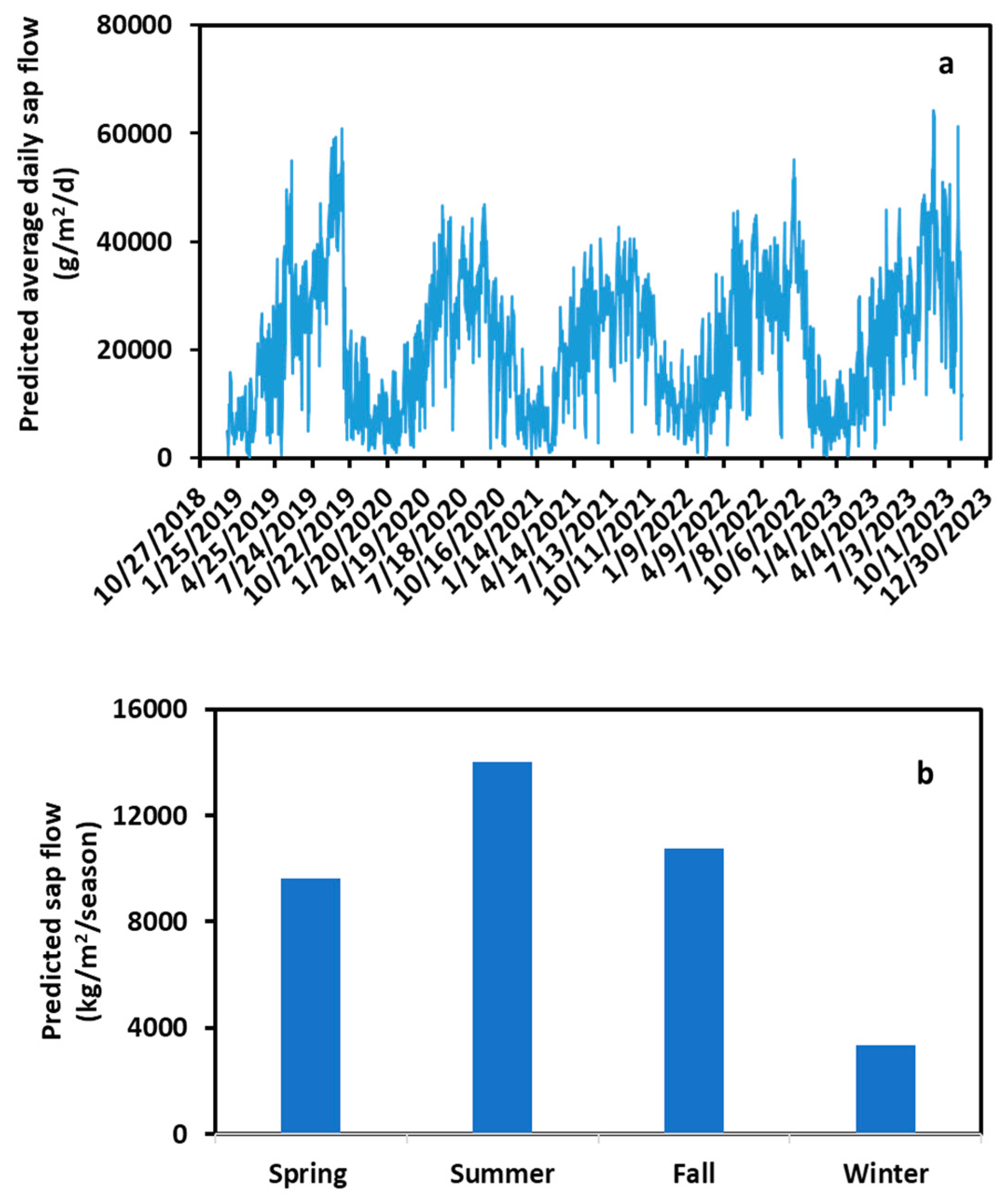
3.3. Multiple Years Sap Flow Prediction

Annual variations of average daily eastern cottonwood sap flow over approximately a 5-year simulation period from 1 January 2019 to 31 October 2023 are presented in Figure 10a. This figure shows a typical annual pattern of sap flow increasing from winter to summer and decreasing from summer to next winter. This annual pattern corresponded well to the annual pattern of air temperature. It is apparent that air temperature is one of the major driving forces for eastern cottonwood sap flow. Additionally, the annual pattern of sap flow was similar to that reported by Samuelson et al. [30]. These authors performed field experiments to estimate the influence of irrigation and fertilization on the sap flow and hydraulic properties of a 3-year-old eastern cottonwood at a 24.4 ha experimental plantation located near Aiken, South Carolina, USA. Our simulations further reveal that the annual average daily sap flow of a tree was 23,038 g/m²/d, which was comparable with that of 25,920 g/m²/d reported by Ouyang et al. [9] at the same study site. The results confirmed that the copula-based regression equation was able to repeat the annual pattern of daily eastern cottonwood sap flow.

Seasonal changes of sap flow over the 5-year simulation period are shown in Figure 10b. The order of sap flow was summer (14,013 kg/m²/season) > fall (10,765 kg/m²/season) > spring (9618 kg/m²/season) > winter (3325 kg/m²/season). In other words, the summer season accounted for 37% and the winter season accounted for 9% of the sap flow, with spring and fall seasons in between.

4. Conclusions

This study develops an approach to predict tree sap flow based on the vapor pressure deficit (VPD) using the copula method in the R-statistics platform. The approach was tested against field-measured data collected with sensors from an eastern cottonwood plantation. A very reasonable agreement was obtained between the copula-predicted and field-measured sap flows, as indicated by the Mann–Kendall and Nash–Sutcliffe efficiency statistics.

The copula-based approach was applied to ascertain eastern cottonwood sap flows at a time when the measured sap flows were unavailable. The results suggest that the copula-based approach is a useful tool for predicting sap flows in a time-saving and cost-effective manner.

It should be noted that the copula-based approach can also be used to predict the sap flows of other tree species. For a specific tree species and study site, users will first need some measured sap flow data to develop a copula-based regression equation between sap flow and VPD by following the steps outlined in Section 2.2.

The copula approach developed here has great potential to predict biomass production based on plant water use and soil nutrient availability in forest management; surface water contamination (e.g., sediment contamination) based on stream discharge in water resource management; and climate change impacts on hydrological processes based on changing air temperature and precipitation.

A major limitation in the application of the copula approach is the need for field-measured data to establish a copula-regression equation between sap flow and VPD for a specific study site. However, this limitation applies to most well-known models such as SWAT (soil and water assessment tool) and HSPF (Hydrological Simulation Program—FORTRAN). To apply the SWAT and HSPF models, users must have field-measured data for model calibrations and validations.

The Kernel density function and machine learning algorithms have been employed to predict plant sap flow. Further study is therefore warranted to compare the copula approach developed here with the Kernel density function and machine learning algorithms for predicting tree sap flow.

References

1. Wullschleger, S.D.; Hanson, P.J.; Tschaplinski, T.J. Whole-plant water flux in understory red maple exposed to altered precipitation regimes. Tree Physiol. 1998, 18, 71–79. [Google Scholar] [CrossRef]
2. Merlin, M.; Solarik, K.A.; Landhausser, S.M. Quantification of uncertainties introduced by data-processing procedures of sap flow measurements using the cut-tree method on a large mature tree. Agric. Forest. Meteorol. 2020, 287, 107926. [Google Scholar] [CrossRef]
3. Oki, T.; Kanae, S. Global hydrological cycles and world water resources. Science 2006, 313, 1068–1072. [Google Scholar] [CrossRef] [PubMed]
4. Ouyang, Y.; Leininger, T.D.; Moran, M. Impacts of reforestation upon sediment load and water outflow in the Lower Yazoo River Watershed, Mississippi. Ecol. Eng. 2013, 61, 394–406. [Google Scholar] [CrossRef]
5. Phillips, N.; Oren, R. Intra- and inter-annual variation in transpiration of a pine forest. Ecol. Appl. 2001, 11, 385–396. [Google Scholar] [CrossRef]
6. Wilcox, B.P.; Breshears, D.D.; Allen, C.D. Ecohydrology of a resource-conserving semiarid woodland: Effects of scale and disturbance. Ecol. Monogr. 2003, 73, 223–239. [Google Scholar] [CrossRef]
7. Liu, X.; Zhang, B.; Zhuang, J.Y.; Han, C.; Zhai, L.; Zhao, W.R.; Zhang, J.C. The Relationship between Sap Flow Density and Environmental Factors in the Yangtze River Delta Region of China. Forests 2017, 8, 74. [Google Scholar] [CrossRef]
8. Nadezhdina, N.; Cermák, J.; Ceulemans, R. Radial patterns of sap flow in woody stems of dominant and understory species: Scaling errors associated with positioning of sensors. Tree Physiol. 2002, 22, 907–918. [Google Scholar] [CrossRef]
9. Wieser, G.; Gruber, A.; Oberhuber, W. Sap flow characteristics and whole-tree water use of across the treeline ecotone of the central Tyrolean Alps. Eur. J. Forest Res. 2014, 133, 287–295. [Google Scholar] [CrossRef]
10. Ouyang, Y.; Leininger, T.D.; Renninger, H.; Gardiner, E.S.; Samuelson, L. A Model to Assess Eastern Cottonwood Water Flow Using Adjusted Vapor Pressure Deficit Associated with a Climate Change Impact Application. Climate 2021, 9, 22. [Google Scholar] [CrossRef]
11. Chen, X.Y.; Miller, G.R.; Rubin, Y.; Baldocchi, D.D. A statistical method for estimating wood thermal diffusivity and probe geometry using in situ heat response curves from sap flow measurements. Tree Physiol. 2012, 32, 1458–1470. [Google Scholar] [CrossRef] [PubMed]
12. Li, Y.; Guo, L.; Wang, J.; Wang, Y.; Xu, D.; Wen, J. An Improved Sap Flow Prediction Model Based on CNN-GRU-BiLSTM and Factor Analysis of Historical Environmental Variables. Forests 2023, 14, 1310. [Google Scholar] [CrossRef]
13. Ouyang, Y. A Hybrid of Copula Prediction and Time Series Computation to Estimate Stream Discharge Based on Precipitation Data. J. Am. Water Resour. Assoc. 2022, 58, 471–484. [Google Scholar] [CrossRef]
14. Sklar, A. Fonctions de Répartition à n Dimensions et Leursmarges; Publications de l’Institut de Statistique de l’Université de Paris: Paris, France, 1959. [Google Scholar]
15. Alizadeh, H.; Mousavi, S.J.; Ponnambalam, K. Copula-Based Chance-Constrained Hydro-Economic Optimization Model for Optimal Design of Reservoir-Irrigation District Systems under Multiple Interdependent Sources of Uncertainty. Water Resour. Res. 2018, 54, 5763–5784. [Google Scholar] [CrossRef]
16. Frees, E.W.; Valdez, E.A. Hierarchical Insurance Claims Modeling. J. Am. Stat. Assoc. 2008, 103, 1457–1469. [Google Scholar] [CrossRef]
17. Genest, C.; Favre, A.C.; Beliveau, J.; Jacques, C. Metaelliptical copulas and their use in frequency analysis of multivariate hydrological data. Water Resour. Res. 2007, 43, W09401. [Google Scholar] [CrossRef]
18. Salvadori, G.; De Michele, C. Frequency analysis via copulas: Theoretical aspects and applications to hydrological events. Water Resour. Res. 2004, 40, W12511. [Google Scholar] [CrossRef]
19. Sun, C.Y. Bivariate Extreme Value Modeling of Wildland Fire Area and Duration. Forest Sci. 2013, 59, 649–660. [Google Scholar] [CrossRef]
20. Cote, M.P.; Genest, C.; Omelka, M. Rank-based inference tools for copula regression, with property and casualty insurance applications. Insur. Math. Econ. 2019, 89, 1–15. [Google Scholar] [CrossRef]
21. Masarotto, G.; Varin, C. Gaussian Copula Regression in R. J. Stat. Softw. 2017, 77, 1–26. [Google Scholar] [CrossRef]
22. Parsa, A.R.; Klugman, S.A. Copula Regression. Var. Adv. Sci. Risk 2008, 5, 45–54. [Google Scholar]
23. Murray, F.W. On the Computation of Saturation Vapor Pressure; Rand Corp.: Santa Monica, CA, USA, 1966. [Google Scholar]
24. Nelson, R.B. Extremes of nonexchangeability. Stat. Pap. 2007, 48, 329–336. [Google Scholar] [CrossRef]
25. Aas, K.; Czado, C.; Frigessi, A.; Bakken, H. Pair-copula constructions of multiple dependence. Insur. Math. Econ. 2009, 44, 182–198. [Google Scholar] [CrossRef]
26. Bedford, T.; Cooke, R.M. Vines—A new graphical model for dependent random variables. Ann. Stat. 2002, 30, 1031–1068. [Google Scholar] [CrossRef]
27. Mangiafico, S. Summary and Analysis of Extension Program Evaluation in R, Version 1. 2023. Available online: https://rcompanion.org/documents/RHandbookProgramEvaluation.pdf (accessed on 10 April 2024).
28. Renard, B.; Lang, M. Use of a Gaussian copula for multivariate extreme value analysis: Some case studies in hydrology. Adv. Water Resour. 2007, 30, 897–912. [Google Scholar] [CrossRef]
29. Vose, J.M.; Swank, W.T.; Harvey, G.J.; Clinton, B.D.; Sobek, C. Leaf Water Relations and Sapflow in Eastern Cottonwood (Populus deltoides Bartr.) Trees Planted for Phytoremediation of a Groundwater Pollutant. Int. J. Phytoremediat. 2000, 2, 53–73. [Google Scholar]
30. Samuelson, L.J.; Stokes, T.A.; Coleman, M.D. Influence of irrigation and fertilization on transpiration and hydraulic properties of Populus deltoides. Tree Physiol. 2007, 27, 765–774. [Google Scholar] [CrossRef]
Figure 1. Location of the Hollandale biomass study site in Mississippi, USA.
Forests 15 00695 g001
Figure 2. Relationship between measured sap flow and VPD (a) and diurnal patterns of the measured sap flow and VPD over a week in spring 2016 (b).
Forests 15 00695 g002
Figure 3. Percentages of maximum peak values for sap flow and VPD occurred in 24 h (a) and their adjustment (b).
Forests 15 00695 g003
Figure 4. Histogram plots of VPD (a) and sap flow (b) data, showing a Gamma type of distribution.
Forests 15 00695 g004
Figure 5. Flow chart used to perform copula analysis.
Forests 15 00695 g005
Figure 6. Comparison of the measured and copula-predicted sap flows and VPDs. The Mann–Kendall’s τ is 0.59 between the predicted and measured sap flows at p < 0.01.
Forests 15 00695 g006
Figure 7. Relationship between the Normal copula predicted sap flow and VPD.
Forests 15 00695 g007
Figure 8. Comparison of the predicted sap flows using the copula regression Equation (4) with the measured sap flows.
Forests 15 00695 g008
Figure 9. Copula predicted hourly sap flows over a growing season (a) and a 2-week period during summer (b).
Forests 15 00695 g009
Figure 10. Copula predicted daily (a) and seasonal (b) sap flows over a 5-year period from 2019 to 2023.
Forests 15 00695 g010