Article

Cold and Wet Island Effect in Mountainous Areas: A Case Study of the Maxian Mountains, Northwest China

1
Key Laboratory of Cryospheric Science and Frozen Soil Engineering, Northwest Institute of Eco-Environment and Resources, Chinese Academy of Sciences, Lanzhou 730000, China
2
University of Chinese Academy of Sciences, Beijing 100049, China
3
China-Pakistan Joint Research Center on Earth Sciences, Islamabad 45320, Pakistan
4
College of Geology Engineering and Geomatics, Chang’an University, Xi’an 710054, China
*
Author to whom correspondence should be addressed.
Forests 2024, 15(9), 1578; https://doi.org/10.3390/f15091578
Submission received: 26 January 2024 / Revised: 11 August 2024 / Accepted: 5 September 2024 / Published: 9 September 2024
(This article belongs to the Special Issue Application of Remote Sensing in Vegetation Dynamic and Ecology)

Abstract

:
The Maxian Mountains, characterized by high altitudes and abundant vegetation, create a cooler and more humid environment compared to the surrounding areas, and are highly susceptible to climate change. In order to study the cold and wet island effects in the Maxian Mountains, air temperature and relative humidity (RH) were analyzed using meteorological station data. Additionally, spatial variations were examined by retrieving Land Surface Temperature (LST) and the Temperature Vegetation Dryness Index (TVDI) from 2001 to 2021. The most pronounced cold island effect was observed in the mountainous area during summer, mainly in May and July. The most significant wet island effect was observed from March to May, with an average relative humidity difference of 24.72%. The cold island area index, as an indicator of the cold island effect, revealed an increasing trend in the summer cold island effect in recent years. The cooling intensity ranged from 5 to 10 °C, with variations observed between 500 and 1000 m. A 30% increase in wet island effects in summer was observed, with a humidification intensity within a range of 500 m. Geodetector analysis identified vegetation cover as the primary factor affecting the thermal environment in mountainous areas. The increase in vegetation in mountainous areas was identified as the main reason for enhancing the cold and wet island effects. The findings emphasize the role of vegetation in enhancing cold and wet island effects, which is crucial for understanding and preserving mountainous regions.

1. Introduction

Mountain ecosystems, particularly those at high altitudes, are critical for maintaining biodiversity, regulating regional climates [1], and providing essential water resources [2], especially in the context of global climate change, which has led to rising temperatures, altered precipitation patterns [3], and increased frequency of extreme weather events such as heat waves and floods [4]. Mountain ecosystems often exhibit distinct cold and wet island effects. These effects are characterized by lower temperatures and higher humidity [5,6], due to vegetation cover and increased precipitation influenced by high-altitude terrain. As a result, the mountains have cooler and more humid conditions compared to the surrounding lowland areas, creating a microclimate that contrasts sharply with the nearby urban environments [7]. Understanding the cold and wet island effects in mountainous regions is vital for developing effective adaptation strategies, mitigating the urban heat island effect, and promoting sustainable development in nearby urban areas.
In recent decades, changes in forest coverage and other land-use types, coupled with increased human activities such as urbanization and deforestation [8], have significantly impacted regional climates [9]. Previous studies have demonstrated that forest ecosystems can cool the surface temperature during the summer through increased evapotranspiration and shading effects [10,11]. However, the specific impacts of these changes can vary widely depending on the region’s unique climatic and topographical conditions [12]. For instance, while tropical regions may experience a cooling effect due to increased evapotranspiration, high-latitude regions often see a warming effect from reduced albedo [13]. In mountainous regions, the cooling and humidifying effects are more pronounced due to the complex interplay between elevation, vegetation, and microclimatic conditions [14,15]. The cold island effect is a localized microclimate phenomenon typically observed in desert oases and lake regions, where temperatures are lower than in the surrounding desert areas due to evaporation and vegetation shading [16,17]. This effect can be found in urban areas, where wetlands and parks help cool the local environment [18,19]. In mountainous regions, the cold and wet island effect arises from high altitudes and dense vegetation, leading to lower temperatures and higher humidity compared to surrounding lowlands and urban areas. This effect plays a crucial role in regulating regional climates and mitigating urban heat islands.
Given the intricate topography of mountainous regions, obtaining meteorological data proves challenging, making the sparse data from meteorological stations especially valuable [20]. The evolution of remote sensing technology has laid the technical groundwork for research in these areas. In addition to conventional ground-based measurements [21], the spatial and temporal distributions of surface temperature at regional and global scales can only be obtained via remote sensing images for surface temperature inversion, which are obtained from satellites [22,23]. Compared with MODIS, ASTER, and other satellites with thermal infrared channels, the spatial resolutions of Landsat are higher, Landsat also has higher accuracy for retrieving small-scale surface temperatures [24]. Several algorithms, such as mono-channel [25], single-channel method [26], and split-window [27], were developed to retrieve LST from remote sensing images. Studies confirm the high level of accuracy attained by using a mono-window algorithm to invert LST in mountainous regions [28,29,30]. The Temperature-Vegetation Dryness Index (TVDI) combines LST and vegetation indices, such as the Normalized Difference Vegetation Index (NDVI), to assess surface moisture conditions [31,32]. Compared to other indices like the Normalized Difference Moisture Index (NDMI), Surface Moisture Index (SMI), Normalized Moisture Index (NMI), and Normalized Difference Infrared Index (NDII), the TVDI offers several advantages. It provides a comprehensive reflection of surface moisture, is suitable for different climates and surface conditions, and effectively captures changes in moisture [33,34]. Additionally, the TVDI is less influenced by factors such as topography. Its data are easily accessible, making it suitable for large-scale and long-term monitoring, and it serves as a valuable tool for drought monitoring and water resource management [35]. Therefore, this study selects the TVDI as a proxy for assessing surface moisture.
Despite extensive research on urban green spaces and their cooling effects [36,37,38], there is a relative lack of studies focusing on the cold and wet island effects in mountainous areas surrounding urban regions [39]. The Maxian Mountains provide an ideal case study for exploring these effects due to their unique climatic conditions and ecological significance [40,41]. This study aims to quantify the cold and wet island effects in the Maxian Mountains from 2001 to 2020 using satellite-derived land LST, the TVDI, and other relevant data. By examining the spatial and temporal variations of these effects, this research will provide valuable insights into the role of mountain ecosystems in regional climate regulation. The findings will enhance our understanding of the environmental dynamics in the Maxian Mountains and inform policy-making for the sustainable management of mountainous regions in the face of global climate change.

2. Materials and Methods

2.1. Study Area

The Maxian Mountains (35°44′ N, 103°58′ E) are situated in Gansu Province, approximately 40 km south of Lanzhou city. The Maxian Mountains stretch for about 30 km in a northwest-to-southeast direction, and reach a peak elevation of 3670.3 m (Figure 1). The area comprises two main units, the Xinglong and Maxian Mountains. It is situated in a transitional zone between three distinct natural geographical areas: the arid inland region in the northwest, the humid monsoon region in the east, and the alpine area of the Northeast Qinghai–Tibet Plateau. The climate in this area is characterized by cold and humid climates, exhibiting features of both plateau and monsoon climates. The annual temperature is −2.3 °C, with an annual maximum of 15 °C and a minimum of −27 °C at the mountain’s peak, and annual precipitation is 491.1 mm [42]. Due to the unique climate and terrain variation, the vegetation in mountainous areas displays clear vertical zoning with increasing altitude (Figure 1d). Below an altitude of 2000 m, the vegetation primarily consists of farmland and herbaceous plants. Between 2000 m and 2200 m, stunted brushwood is predominant. From 2200 m to 3000 m, the area is characterized by the presence of arbors as the dominant vegetation. Above 3500 m, alpine meadows dominate the landscape, with permafrost confirmed to be present. The persistence of permafrost in the Maxian Mountains is largely attributed to the presence of abundant underground ice, the protection provided by thick organic matter, and a cold microclimate [43].

2.2. Data and Preprocessing

The data used in this study include Landsat 5 TM and Landsat 8 OLI/TIRS from the USGS website (https://earthexplorer.usgs.gov/, accessed on 2 December 2023) for retrieving LST which were resampled to 30 m using data provided by NASA. Mean compositing was applied to summer and annual images. This approach not only addresses uncertainties arising from transient images but also mitigates cloud coverage in imagery of mountainous regions. The elevation data were obtained from the Global Digital Elevation Model (ASTER GDEM) with a spatial resolution of 30 m (https://search.earthdata.nasa.gov/, accessed on 10 October 2023) (Table 1).
The land use data used are derived from the 30 m National Annual Land Cover Data CLCD (V1.0.2) released by Wuhan University. This dataset includes the 2022 national land cover data (https://doi.org/10.5281/zenodo.4417810, accessed on 1 Septembert 2023), spanning from 1986 to 2022 and provides yearly land cover information for China. The dataset includes nine major land use categories: farmland, forest, shrub, grassland, water, ice and snow, wild land, impervious surfaces, and wetlands (Table 1).
The precipitation data in this article were obtained from ERA5 provided by the European Centre for Medium-Range Weather Forecasts (ECMWF). The data have a temporal resolution of 1 h, spatial resolution of 0.05°, and cover the period from 2001 to the present (Table 1).
Two automatic meteorological observation stations were established in the study area in 2009. The main parameters include air temperature, wind speed, relative humidity, net solar radiation, soil heat flux, etc., with a data acquisition interval of 30 min. The distance between the two meteorological stations is less than 100 m, so for the missing data, the two meteorological stations on the top of the mountain complement and interpolate each other. Additionally, data from one national meteorological station were obtained from the China Meteorological Data Service Center (http://data.cma.cn, accessed on 28 August 2023) (Table 2).

2.3. Methodology

2.3.1. Land Surface Temperature Retrieval

This study employed the mono-window algorithm proposed by Qin [25] to retrieve LST from Landsat 5 TM/8 TIRS (https://earthexplorer.usgs.gov/, accessed on 2 December 2023). The specific algorithms are as follows:
T s = 1 C × a × 1 C D + b × 1 C D + C + D × T s e n C × T a
C = ε × τ
D = 1 τ × 1 + 1 ε × τ
where Ts is the surface temperature, and T s e n is the brightness temperature observed by the sensor, and Ta is the average atmospheric temperature, where the value of a is −67.355351 and b is 0.458606., and ε is the surface emissivity, and τ is the total atmospheric transmittance.
ε = 0.979 0.035 ρ r e d ; N D V I < 0.2 0.986 + 0.004 N D V I N D V I s / N D V I V N D V I s 2 ; 0.2 N D V I 0.5 0.99 ; N D V I > 0.5
The average temperature of the atmosphere mainly depends on the temperature distribution of the atmospheric profile and the state of the atmosphere. However, obtaining real-time atmospheric profile data and atmospheric state data can be challenging due to the limited time that satellites spend flying over the study area. This paper employs an estimation method to determine the average temperature of the atmosphere during mid-latitude summers. It specifically examines the relationship between the average temperature of the atmosphere temperature (Ta) and the near-surface temperature (T0) used. By obtaining the temperature data of the meteorological station for nearly 2 m, it is concluded that Ta:
T a = 16.0110 + 0.9262 × T 0
The atmospheric transmittance of the study area was estimated by using the relationship between atmospheric transmittance and water vapor content. This was carried out by considering the atmospheric transmittance in mid-latitude summer. Additionally, the water vapor content was obtained using the MODIS water vapor product data.
τ 6 = 0.08007 × ω + 0.97429
τ 10 = 0.0725 × ω + 0.9184
where τ6 and τ10 are the atmospheric transmittance for the TM band 6 and TIRS band 10, respectively, and ω presents the atmospheric water vapor content.

2.3.2. Ts-NDVI Model

The Ts-NDVI characteristic spatial model estimates soil moisture by utilizing a combination of various inputs and methodologies. The TVDI value ranges from 0 to 1, with smaller values indicating wetter surface conditions [32]. The TVDI model and the equations for the dry/wet edges are calculated as follows:
T V D I = T s T s min T s max T s min
T s max = a + b × N D V I
T s min = c + d × N D V I
where Ts is the surface temperature of any image element; T S m a x is the maximum surface temperature corresponding to NDVI, representing the dry side; T s m i n is the minimum temperature corresponding to NDVI, representing the wet side; and a and b represent the intercept and slope of the dry edge, respectively. Similarly, c and d represent the intercept and slope of the wet edge, respectively.

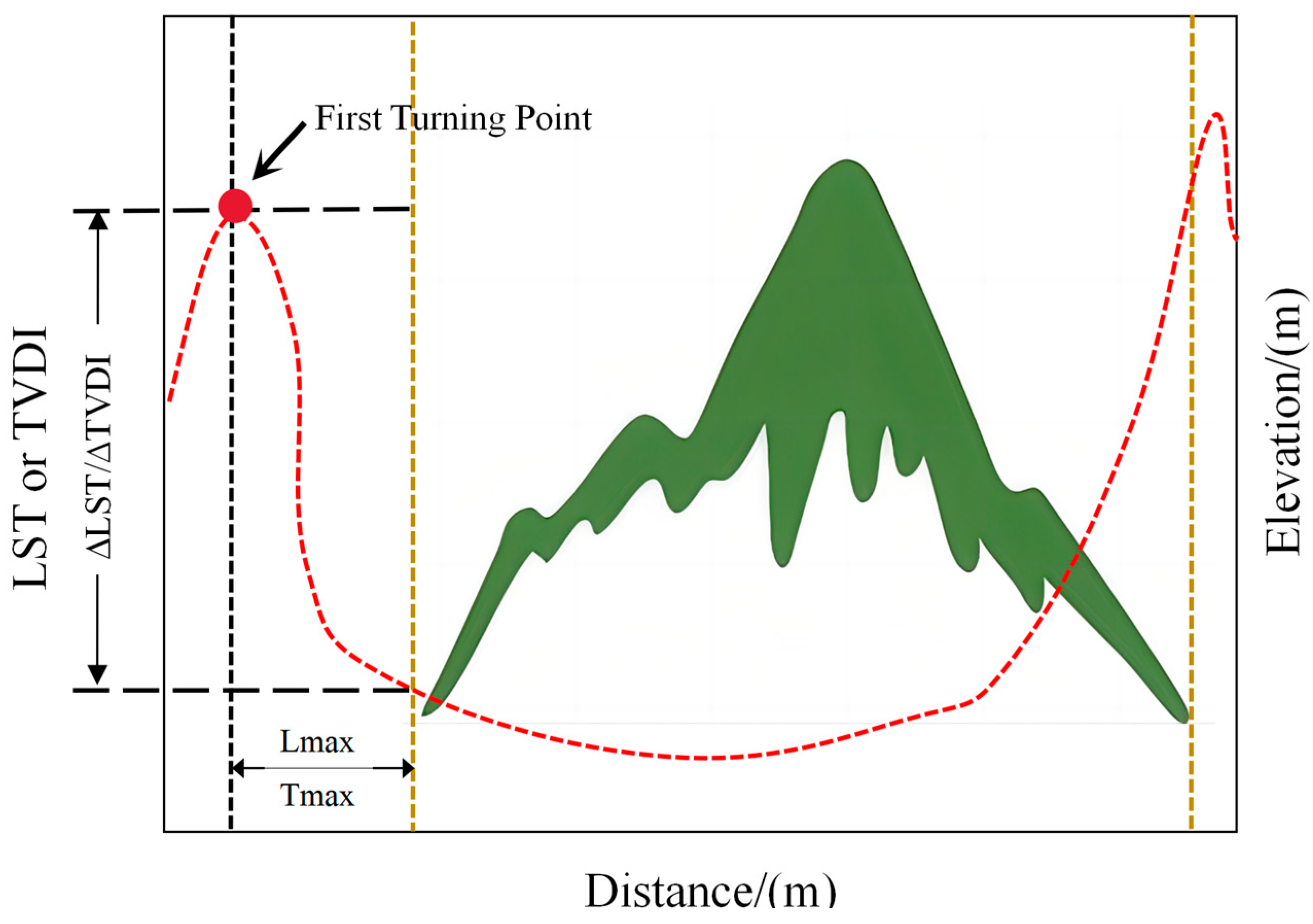
2.3.3. Cold and Wet Island Index Calculation

The definition of the cool island effect in urban green spaces and water bodies was used to establish the concept of the cold and wet island effect in mountainous regions [44]. This effect refers to the occurrence where the LST and TVDI values in the mountainous area are lower (higher) than those of the surrounding environment. The intensity of the cold and wet island effect is determined by two components: cooling distance (km) and cooling magnitude (°C) [45], similarly, the variation in TVDI reflects the moisture conditions associated with this effect (Figure 2).
Due to the resolution limitations of Landsat imagery, we calculated the mountain boundaries by determining the terrain roughness through ArcGIS. Subsequently, these boundaries were imported into Google Earth Pro 7.3.6.9796 for manual visual inspection, relying on green areas to accurately delineate the mountain’s vector boundaries.
The maximum extent of the mountainous cold–wet island effect is defined as the distance between the edge of the mountainous area and the first inflection point where temperature and humidity begin to decrease. This distance is commonly referred to as the range of the mountainous cold island effect. The difference in temperature and humidity between these two points is known as the magnitude of variation in the cold–wet island effect. To further analyze this effect, we selected profile lines in different directions across the mountainous area and examined the average LST and TVDI values on both sides of these profile lines.
This study utilizes the cold and wet island index to conduct a comparative analysis of remote sensing data at different time periods and to quantitatively evaluate changes in the phenomenon of cold and wet islands effect. Similarly, the same calculation method is applied to the Wet Island Index [46]:
C I I = 1 100 m i = 1 n w i × p i
where CII is the cold island index; m is the LST or TVDI classification level, with LST being divided into five grades for the cold island effect, and TVDI into five grades for the wet island effect; so, in both cases, m = 5; i is the temperature level in the urban area lower than that in the suburban area; n is the number of LST (TVDI) in lower (higher) level; w is the weight value, which takes the level value of the i level, and p is the percentage of the i level.

2.3.4. Grading Method of LST and TVDI

When comparing LST at different times, the varying imaging times of remote sensing images result in significant variations in the maximum and minimum values of the retrieved LST. Additionally, anomalous temperature values make direct comparative analysis inconvenient. Therefore, it is necessary to normalize the images for accurate comparison. Subsequently, similar to the methods used for grading an urban heat island, the mean-standard deviation classification method is applied to categorize it into five classes [47]. For the TVDI grading method, an equal interval classification is employed with intervals of 0.2 [33], resulting in five classes as shown in Table 3.

2.3.5. Geodetector Model

Geodetector (2015) is a novel statistical method that is widely used to study spatial heterogeneity and identify the underlying driving factors, especially in research that focuses on geographic environmental effects [48]. Compared to geodetector, correlation and regression analyses are commonly used in existing studies. However, there is a lack of quantitative analysis of multiple factors and their interactions. In contrast, using geographic detectors offers a new research approach by detecting spatial heterogeneity in geographic phenomena. This, in turn, reveals potential interactions among multiple factors [49]. This study utilizes the geodetector model functions including [50]: (1) Factor detection, which detects the degree of explanation of the independent variable on the dependent variable. The q values are expressed as follows:
q = 1 1 N σ 2 h = 1 L N h × σ h 2
where h is the classification of factors affecting the distribution of surface temperature and humidity; h is the number of cells of h and N is the total number of cells in the study area; and σ are the variance of a layer of the variable and the variance of the whole area, respectively. As surface temperature and humidity are the result of the combined effect of several factors, a higher q value indicates that the influencing factors can more suitably explain the spatial variance of surface temperature and humidity, whereas lower q values indicate the opposite.
Interactive detection: Interaction detection can identify the interaction between different risk factors, and evaluate whether the combined action of factors X1 and X2 will increase or decrease the explanatory power of the dependent variable Y, or whether the effects of these factors on Y are independent of each other (Table 4).

3. Results

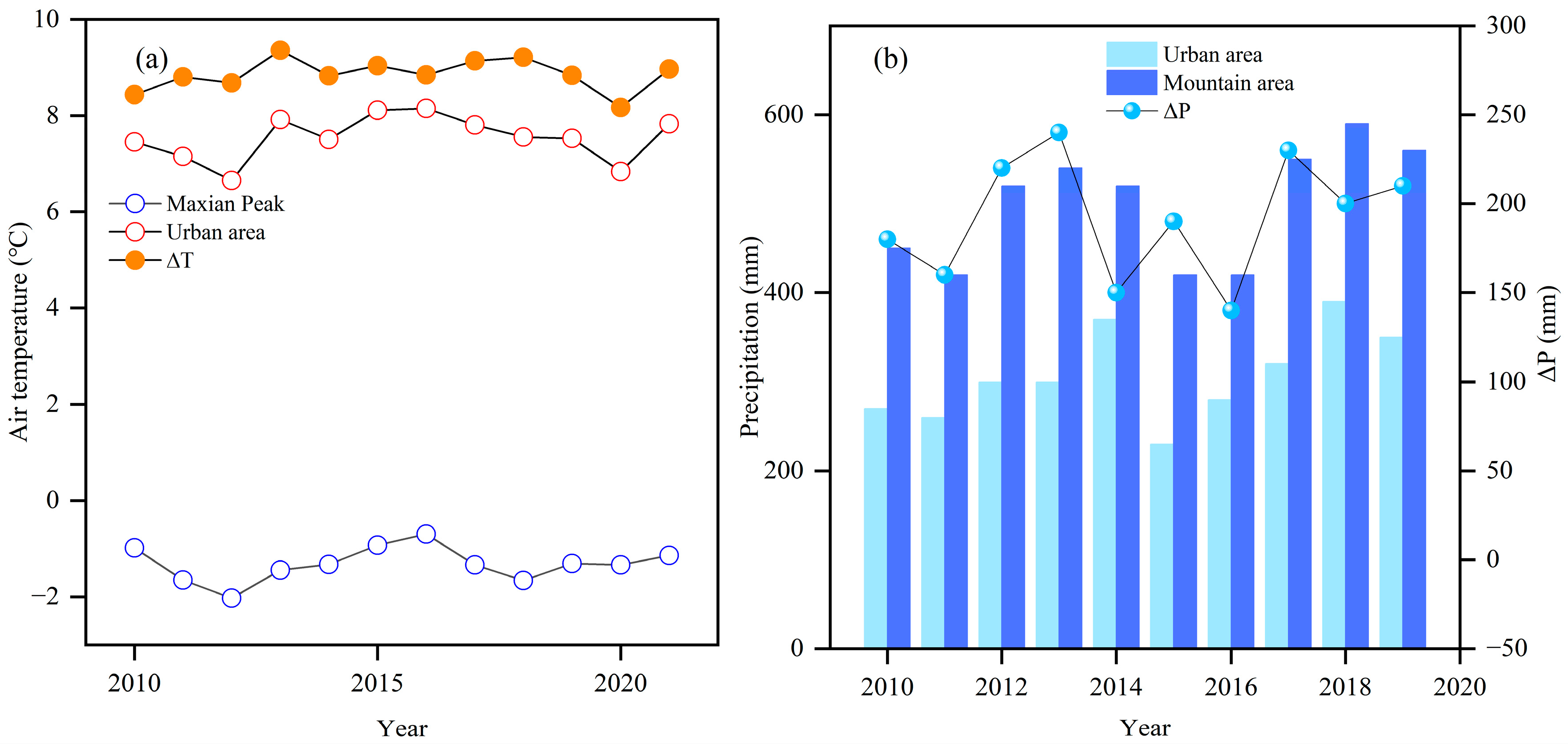
3.1. Annual Variations in Precipitation and Air Temperature

Figure 3 depicts the yearly air temperature and precipitation in the Maxian Mountains and the surrounding urban area for the period of 2010 to 2021. The average annual temperature in the Maxian Mountains fluctuated between −2.02 °C and −0.69 °C. Conversely, in the urban area, the annual average temperature ranged from 6.65 °C to 8.14 °C. The temperatures in the mountainous and urban areas differ by approximately 9 °C annually.
Due to the limited availability of precipitation data for the mountainous area, ERA5 reanalysis data from 2010 to 2019 were used. The annual average precipitation in the mountainous areas was significantly higher compared to the urban areas, with variations ranging from 140 mm to 240 mm. Notably, the mountainous area has experienced an upward trend in precipitation in recent years, peaking at 590 mm and dropping to a minimum of 420 mm. Conversely, the urban area has experienced fluctuating annual precipitation within the range of 230 mm to 390 mm (Figure 3b).

3.2. Monthly and Daily Changes in Air Temperature and Relative Humidity

3.2.1. Analysis of Air Temperature Variations on Monthly and Daily Scales

Figure 4a shows the annual air temperature difference between 2015 and 2020. In the urban area, temperatures range from below 0 °C in December to March and reach a peak of 24 °C in August, then dropping to −8 °C in mid-December. The annual temperature difference is approximately 32 °C. The temperature trends in the mountains closely resemble those in the urban area, with a peak of 12 °C in August and a minimum of −15.2 °C from mid-December to mid-January, resulting in an annual temperature range of around 27 °C. The mountainous region experiences a thawing period from May to late October, with temperatures below 0 °C for more than half of the year.
Figure 4b illustrates the temperature lapse rate (TRL) between urban weather stations and mountain summits. It shows that during the summer, the TLR in the mountains is higher compared to the standard atmospheric lapse rate of 0.65 °C/km. Specifically, from May to July, the average TLR is approximately 0.75 °C/km. To account for altitude differences, a standard lapse rate of 0.65 °C/km was used. This adjustment revealed an average cold island effect intensity of roughly 1.69 °C, with a maximum of 5.51 °C. It is hypothesized that this phenomenon may be attributed to factors such as high vegetation coverage, increased evaporation, and reduced heat absorption and radiation in the mountains [51,52]. In contrast, during autumn and winter, the TLR is smaller. This could be attributed to reduced solar radiation, slower ground cooling, and the presence of snow, which enhances surface reflectivity and reduces heat absorption [53].
Analysis of daily temperature variations in different seasons (Figure 4c) shows the largest differences in summer and spring, with an approximate difference of 15 °C. In autumn and winter, the variations are more modest. Temporally, temperatures increase from 6 AM, reach their peak around 4 PM, and gradually decrease. The summit has minor daily temperature fluctuations, around 5 °C, while the urban area experiences more significant variations, exceeding those of the summit by more than double. The maximum daily temperature difference in spring is 15 °C.

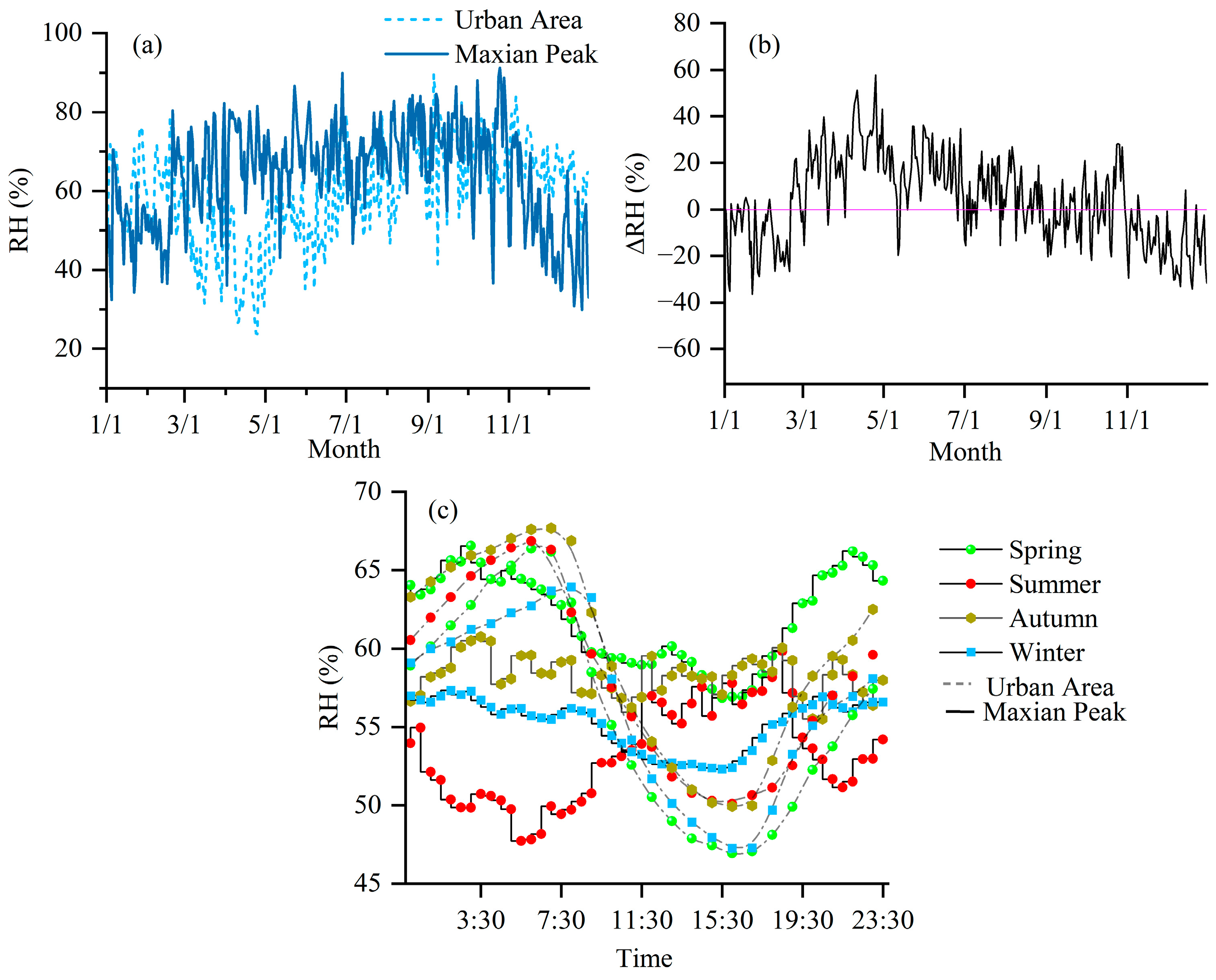
3.2.2. Analysis of Relative Humidity Variations at Monthly and Daily Scales

The analysis of RH disparities between the summit and urban area reveals clear patterns in Figure 5a,b. The mountainous region consistently maintains an average annual RH of around 70%, which is consistently lower than that of the urban area from November to late February. This discrepancy can be attributed to the presence of snow cover, which acts as a thermal insulating layer, leading to lower surface temperatures and restricted surface evaporation. The colder temperatures and insulating layer reduce transpiration, primarily influenced by the snow cover at the summit. In contrast, from March to July, the mountainous RH exceeds that of the urban area, with a maximum difference of 50% and an average relative humidity difference of 24.72%. Between July and November, the disparities in humidity diminish.
Figure 5c depicts the notable daily variations in relative humidity (RH) between mountainous and urban areas. In the urban area, RH is around 65% at approximately 6 AM, with the highest values occurring in autumn. The lowest relative humidity, around 50%, is observed at about 4 PM, resulting in a daily humidity difference of 15%. In the mountainous area, RH fluctuates around 58% between 9 AM and 6:30 PM throughout the seasons, with spring experiencing the highest humidity levels. The maximum difference in RH occurs between 11:30 AM and 6:30 PM, reaching a high of 34.8%. This can be attributed to the summit’s exposure to wind, which leads to moisture loss during this period. Furthermore, the mountainous terrain facilitates the downhill movement of cold air at night, further reducing relative humidity. Conversely, relative humidity variations are minimal in autumn and winter.

3.3. Spatiotemporal Variation Characteristics of LST and TVDI in Mountainous Area

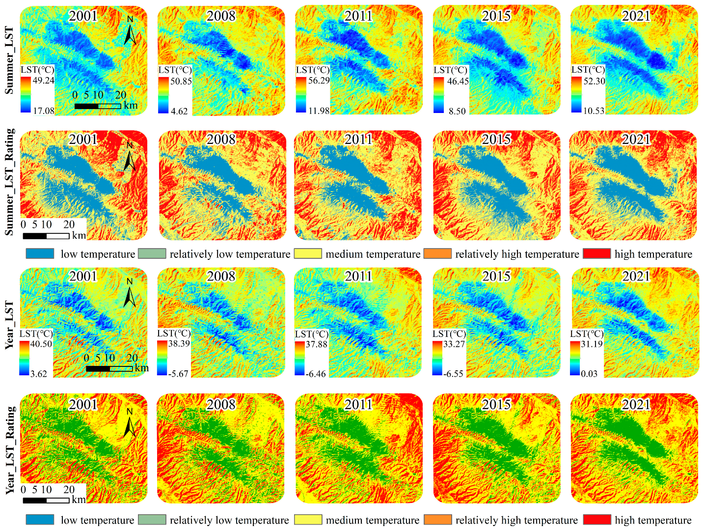
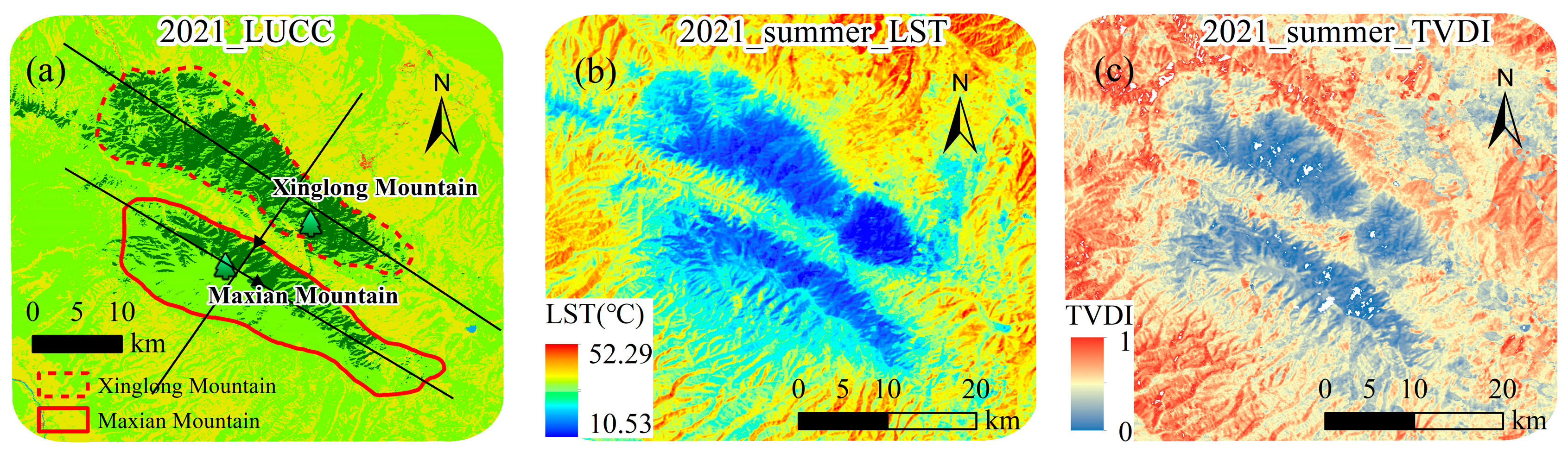
3.3.1. Spatial Distribution Characteristics of LST

By synthesizing the average images from Landsat 8 and Landsat 5 captured between 2001 and 2022, we analyzed the LST during the summer and annually for the years 2001, 2008, 2011, 2015, and 2021. As shown in Figure 6, the mountainous region exhibits distinct zones of low, medium, and high temperatures during the summer season. Similarly, for the annual LST, the distribution is primarily concentrated in areas with low, medium, and high temperatures. The average summer LST in the study area is approximately 31.5 °C, with a temperature difference of about 40 °C. When considering the average annual LST, we find that the average annual LST is 17.21 °C, with a temperature difference of approximately 30 °C. Notably, the mountainous region stands out as a significant “cold island” compared to the surrounding areas.
To analyze the relationship between LST and altitude in the Maxian Mountains, a study was conducted using contour lines at 50 m intervals from the base to the summit. By examining the LST at each 50 m interval, patterns of LST variation with altitude were identified during the summer season and over the years in mountainous area (Figure 7). It indicates that below an altitude of 3400 m, the LST decreases as altitude increases. On average, there is a temperature drop of 1.3 °C per 100 m. However, above 3400 m, a distinct increasing trend in LST. This may be attributed to the presence of a thick peat layer and shallow depression, which act as a thermal insulation layer at the mountain’s peak. Considering the average annual variation of LST with altitude, in the lower altitude range of 2200–2800 m, the temperature decreases as altitude increases. On average, the cooling rate is 0.81 °C per 100 m. Beyond this range, the ground temperature changes more gradually with altitude, showing a decreasing trend at 3400 m.
Based on Figure 8, it is evident that the summer cold island index in mountainous areas has been increasing in recent years. This is mainly attributed to the expansion of the cold zone, leading to considerably lower LST during the summer compared to the surrounding areas. However, when considering the annual fluctuations in the cold island index, there is an overall declining trend, which suggests that the extent of hot zones in mountainous regions is expanding.

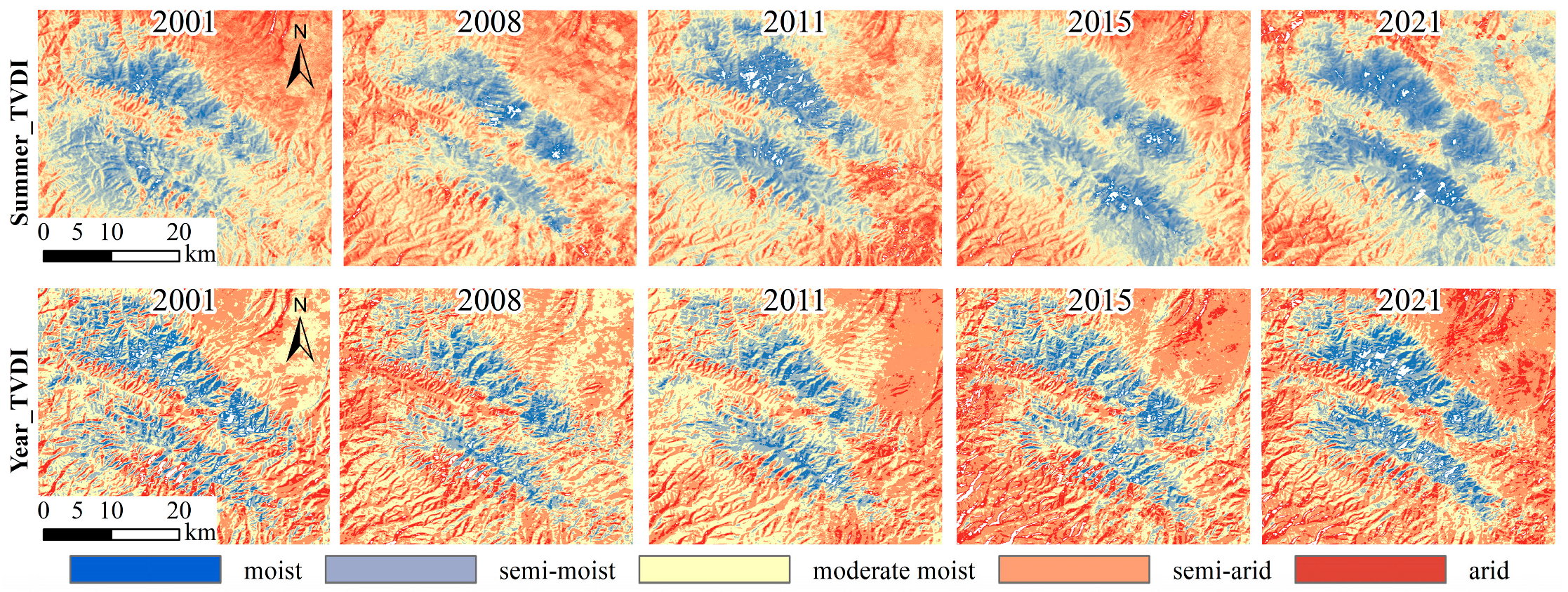
3.3.2. Spatial Distribution Characteristics of TVDI

The TVDI model was used to estimate the soil moisture in the study area. The variation of TVDI in summer and between the of years 2001 and 2021 was calculated separately (Figure 9). The practical value of the TVDI ranges from 0 to 1, divided into moist, semi-moist, moderately moist, semi-arid, and arid regions. Figure 9 reveals that the study area is predominantly characterized by humid and relatively arid areas, with Xinglong Mountain having higher humidity than Maxian Mountain and the Northern Slope of Maxian Mountain having higher soil moisture than the southern slope. Analyzing the proportion index of wet island area change (Figure 10) indicates a significant upward trend in the wet island index in mountainous areas in recent years, primarily in semi-moist areas.

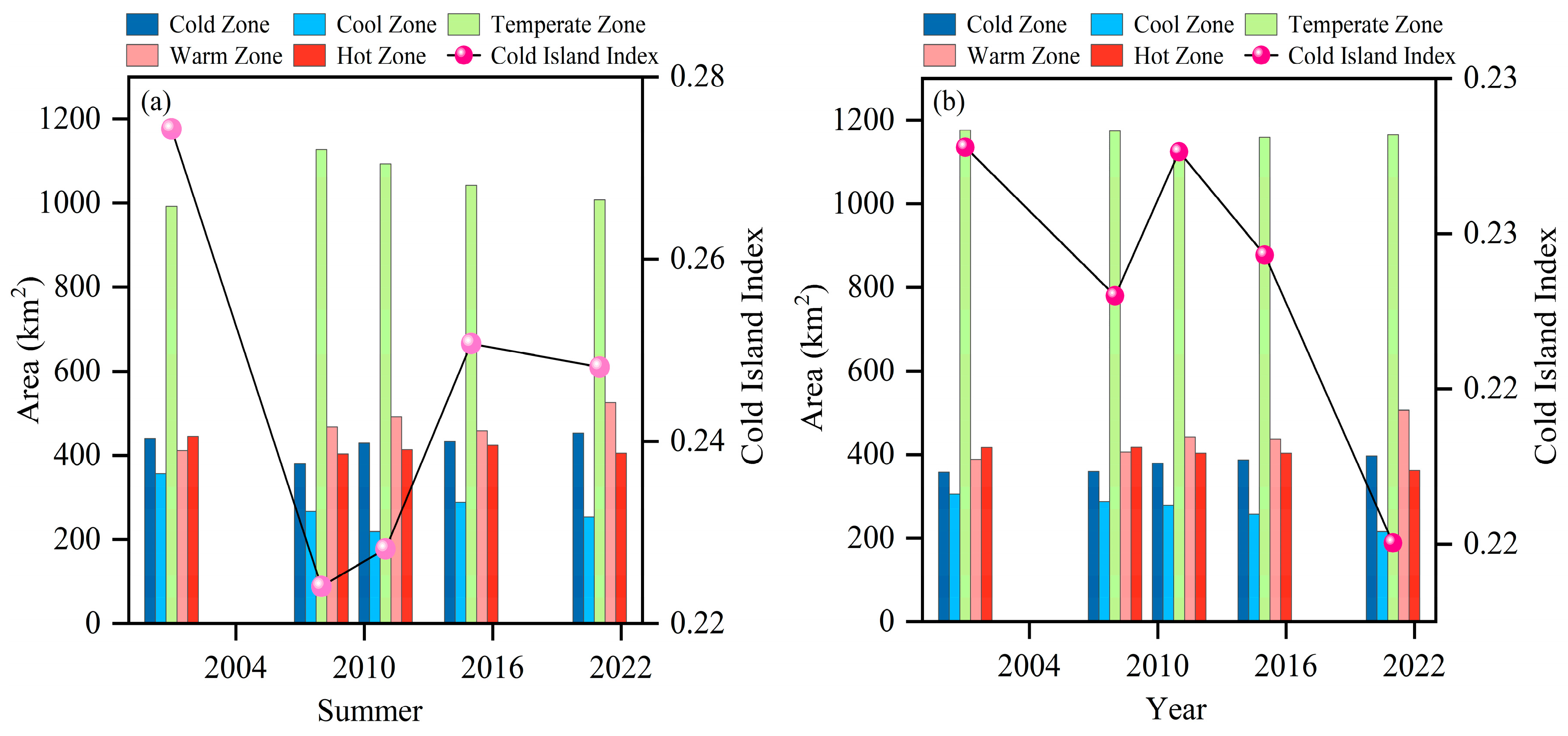
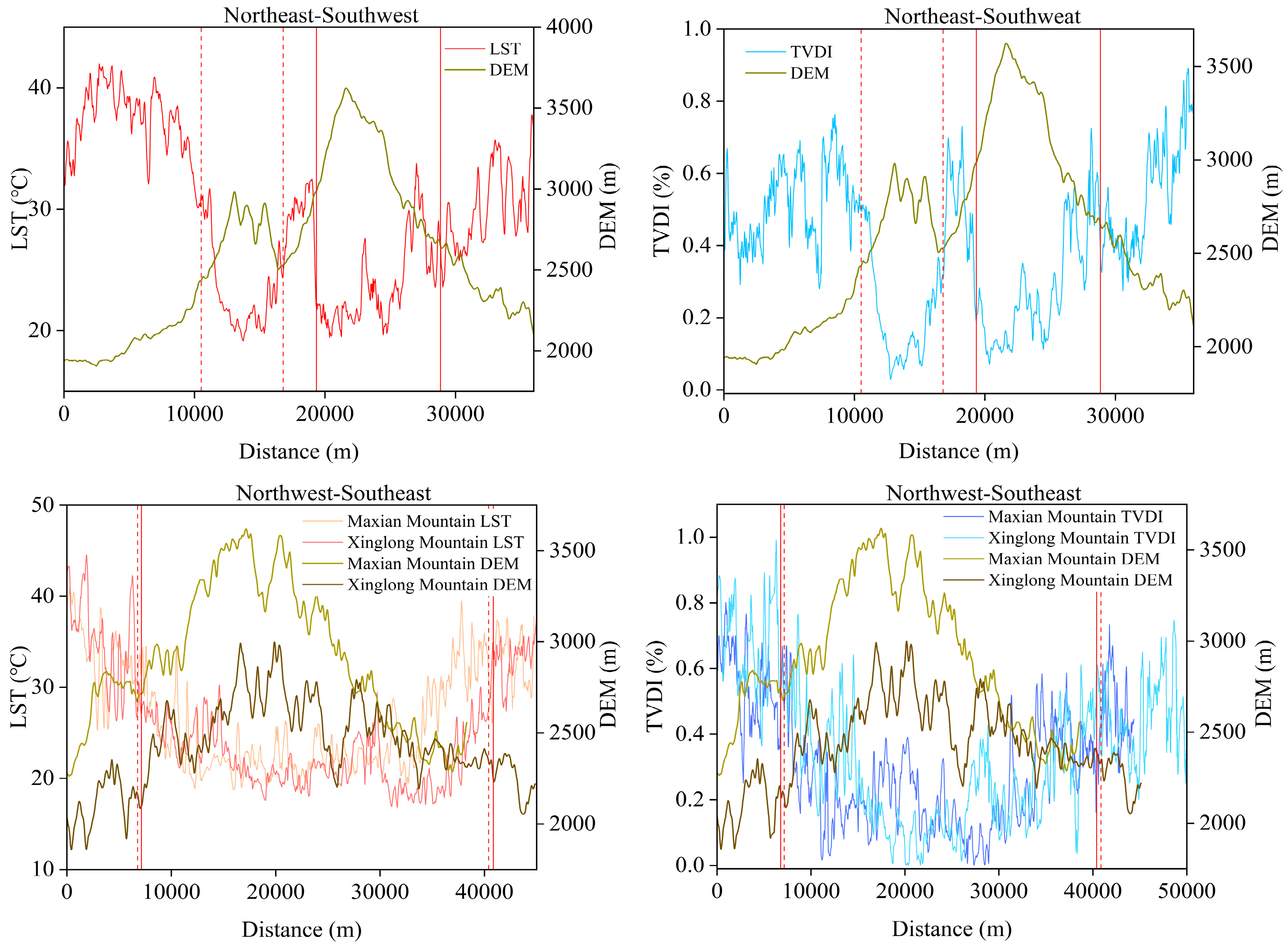
3.4. Analysis of the Cold and Wet Island Effect

We utilizied ArcGIS 10.7 to calculate the terrain fluctuation in mountainous regions, extracting the boundaries of the mountainous areas, and importing them into Google Earth Pro 7.3.6.9796 to identify and select the boundaries of the mountainous terrain. To analyze temperature and humidity in different types of land covers, we conducted a comparison of LST and the TVDI across various land use types. As illustrated in Figure 11, the LST follows the order of wildland > impervious surface > farmland > water body > shrub > forest. In addition, the TVDI for different land use types is ranked highest to lowest as shrub > forest > barren land > impervious surface > grassland > farmland. Furthermore, the surface temperatures also exhibit the same order of wildland > impervious surface > farmland > water > shrub > forest.. The profiles of summer LST and the TVDI maps for the year 2021 were generated along the northeast–southwest and northwest–southeast directions (Figure 12). Meanwhile, a comparative analysis was conducted to assess the strength of the cold and wet island effects between Xinglong Mountain and Maxian Mountain (Figure 13).
After analyzing the cross-sectional profiles in different directions and calculating the intensity of cold island and wet island effects in mountainous areas, the following findings were determined: In the northeast to southwest direction, Xinglong Mountain experiences a temperature reduction of approximately 5 °C. This cooling effect spans a range of 732 m and is accompanied by a 32% increase in humidity, with a humidification range of 563 m. Maxian Mountain exhibits a temperature reduction of 8.7 °C and has a cooling range of 445 m. The humidity increases by 21% within a humidification range of 550 m Xinglong Mountain demonstrates a substantial temperature reduction of about 12.36 °C in the northwest to southeast direction. This cooling effect covers a range of 457 m and is accompanied by a 20% increase in humidity within a humidification range of 446 m. Similarly, Maxian Mountain experiences a temperature reduction of 5.83 °C. The cooling range measures 719 m, while the humidity increases by 34% within a humidification range of 780.5 m.

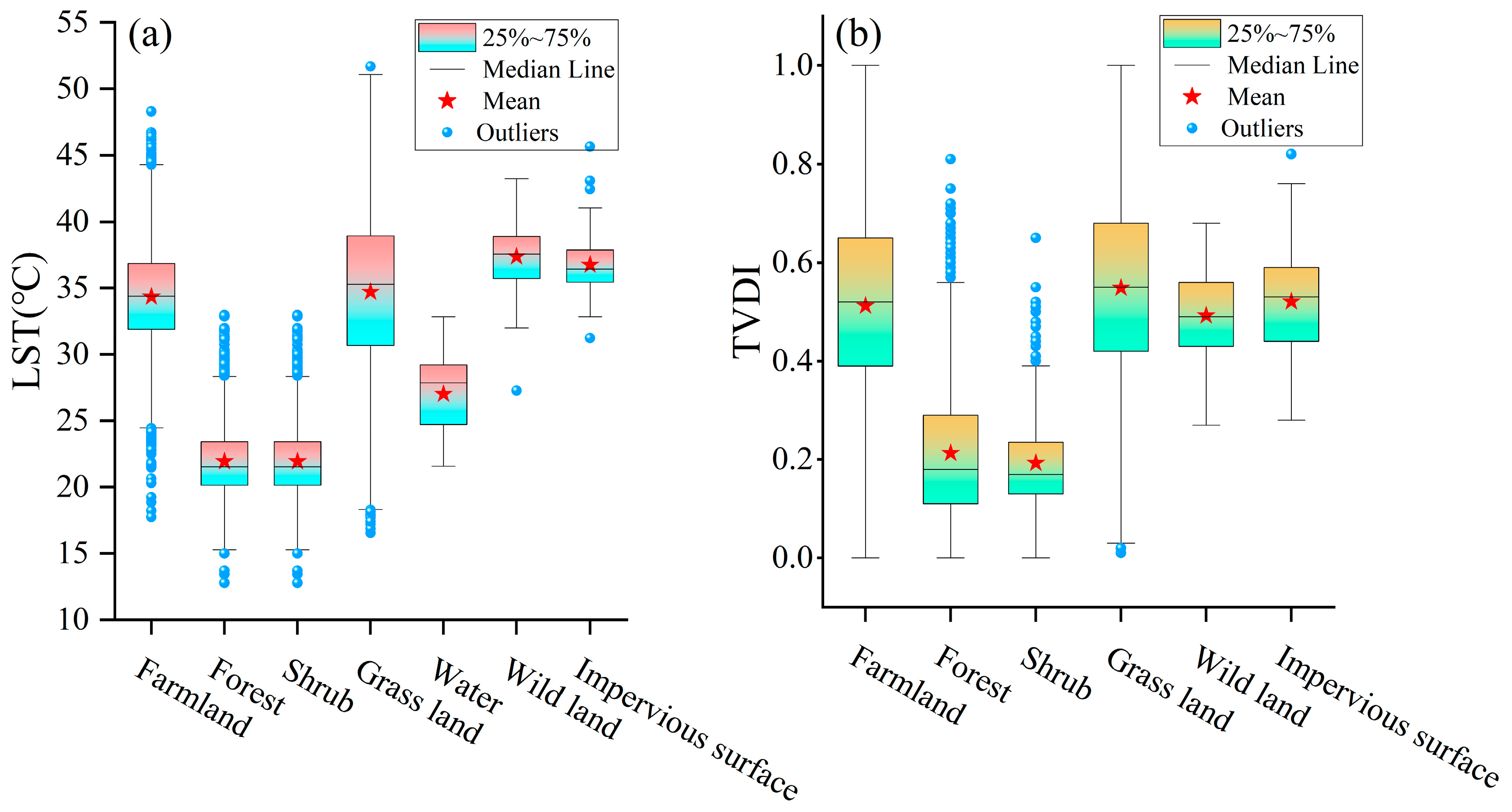
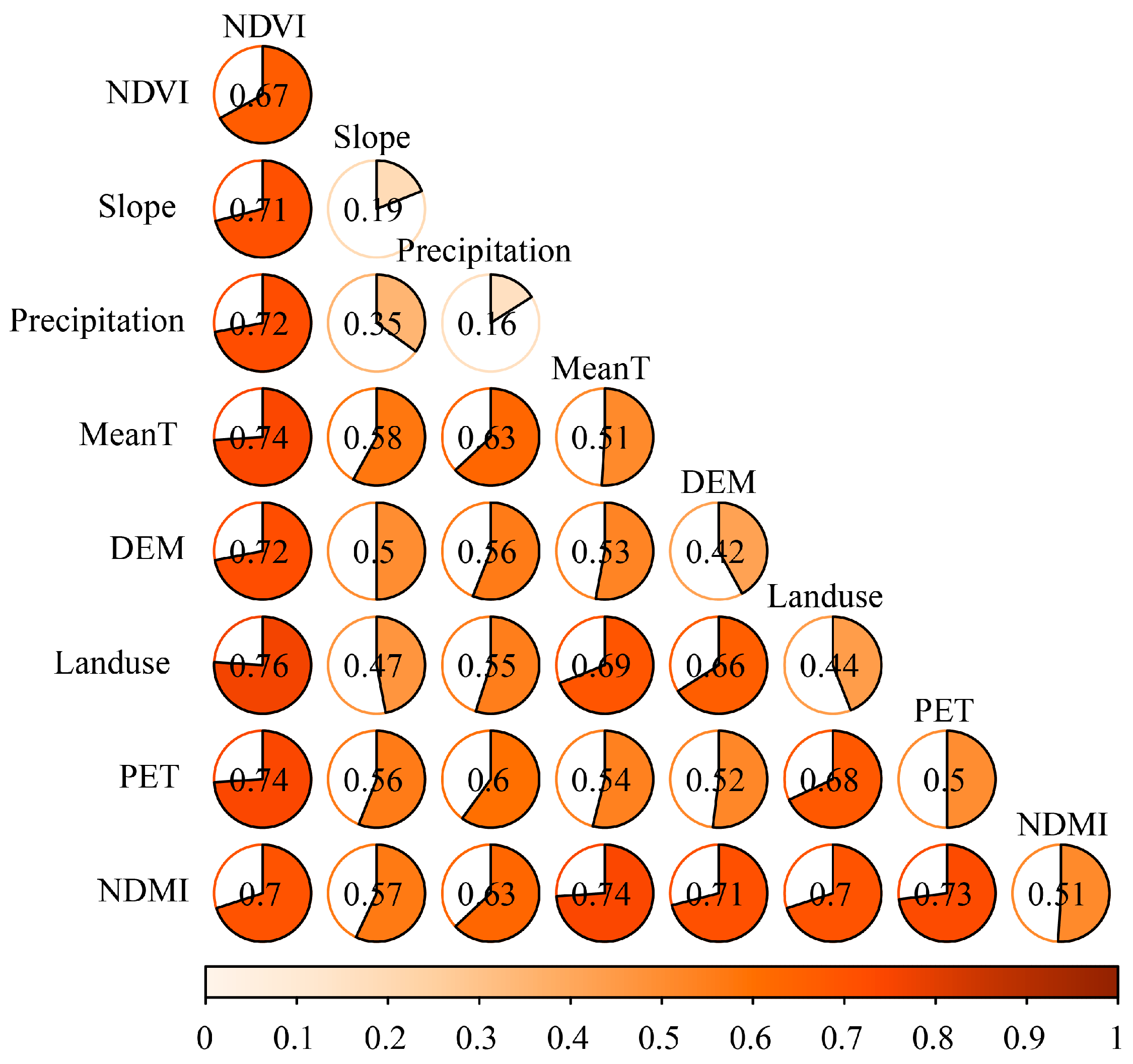
3.5. Influencing Factors for the LST

In order to investigate the factors that influence the thermal environment of the land surface in mountainous areas with minimal human interference, we selected eight natural factors NDVI, Slope, Precipitation, Mean Temperature, DEM, Land use, Potential Evapotranspiration (PET), Normalized Difference Moisture Index (NDMI)) based on previous research. These factors were chosen to analyze the impact of different variables on LST. All eight factors have passed the significance level test at 0.01 (Table 5). The order of explanatory power for each influencing factor on LST is as follows: NDVI (0.67) > NDMI (0.52) > MeanT (0.509) > PET (0.503) > Landuse (0.44) > DEM (0.42) > Slope (0.19) > Precipitation (0.16). This suggests that vegetation cover is the main driver influencing LST in mountainous areas, followed by NDMI and PET. It emphasizes the significance of vegetation transpiration as the primary factor for surface cooling. Based on the results of interaction detection (Figure 14), two types of interaction effects on mountainous LST are observed: two-factor enhancement and nonlinear enhancement. The dominant type is two-factor enhancement. This suggests that, in most cases, the combined effects of multiple factors on LST are more significant than the effects of individual factors alone. It is important to note that the explanatory power of interactions between NDVI and NDMI with various factors is noticeably higher compared to that of single factors. This indicates that vegetation and water vapor indirectly impact LST.

4. Discussion

This study systematically analyzes the cold and humid climate characteristics of the Maxian Mountain area using meteorological station data and remote sensing methods. It contrasts the climate differences between the mountainous region and the surrounding urban areas. However, due to the limited size of the study area, challenges in acquiring remote sensing images for the mountainous region, and insufficient continuity in the study period, there is a notable limitation in the lack of discussion and research on the spatial variation of nighttime temperature and humidity in the mountainous area.

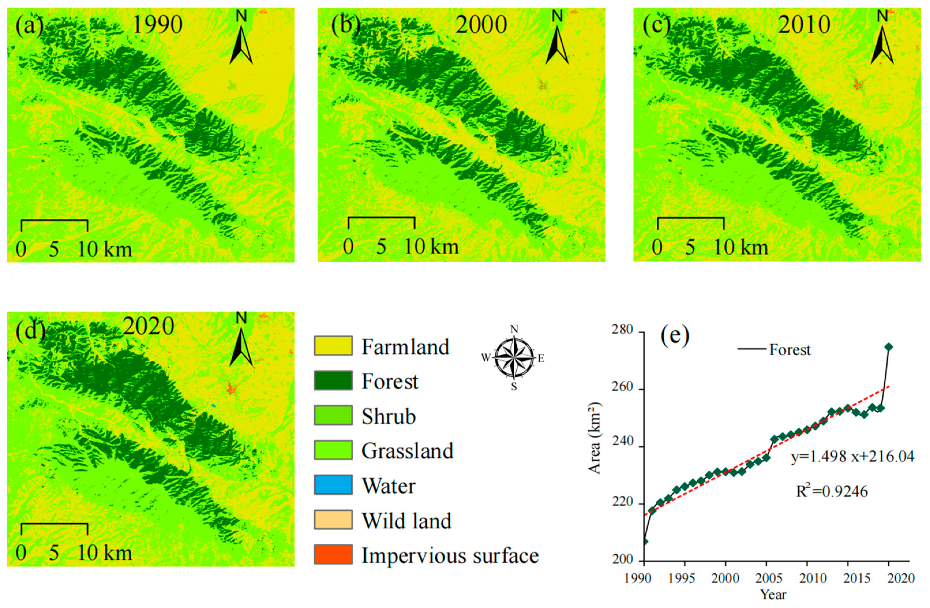
4.1. Impacts of Land Use Changes on the Cold–Wet Island Effect

The transpiration effect of vegetation in mountainous areas significantly influences the cold and humid island effect during the summer. However, urban development in the surrounding areas may contribute to rising LST. An analysis of land use changes in mountainous regions from 1990 to 2020 (Figure 15) showed that the forest area in the mountains shows a yearly increase at a rate of 1.498 km2/a. This may be associated with the rise in mountainous temperatures. Increasing vegetation is crucial in maintaining a relatively cool and moist mountain environment. The temperature may accelerate the thawing of permafrost over the years [54]. Therefore, while strengthening the protection of the Maxian mountainous area, it is essential to develop mountain resources sensibly, ensuring the simultaneous protection of the mountainous ecological environment. Our investigation reveals that, as temperatures show a slight upward trend, the mountainous areas benefit from local government protection, effectively minimizing human activities’ impact on the natural environment [55].

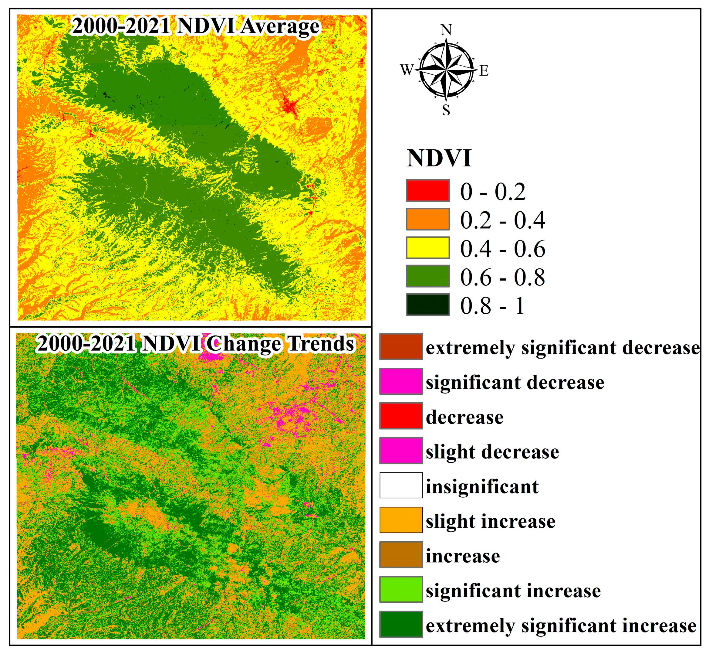
4.2. Characteristics of Vegetation Change in Mountainous Area

The NDVI is a measure used to assess the level of greenness and vegetation growth in a specific region. It plays a crucial role in determining LST and the local climate. In mountainous areas, vegetation coverage is strongly influenced by altitude. As altitude varies, the composition and diversity of vegetation change, leading to distinct vertical zones of vegetation [56]. Additionally, mountainous regions, characterized by their unique topography and climatic conditions such as ample precipitation and low temperatures, create ideal circumstances for the growth of vegetation [57].
By analyzing the distribution characteristics and trend of the NDVI in mountainous areas from 2000 to 2021 using the Mann–Kendall test (Figure 16), we can see that there are spatial variations in vegetation distribution in these areas. The NDVI values in mountainous regions range from 0.6 to 0.8, indicating a high level of vegetation coverage. Specifically, Xinglong Mountain has a higher vegetation coverage compared to Maxian Mountain, with the latter concentrated mainly on the northern slope. Additionally, vegetation in mountainous areas shows an upward trend that weakens as altitude increases. However, beyond an altitude of 3400 m, such as with Maxian Mountain, the changes in vegetation are minimal. On the other hand, the surrounding urban areas are experiencing a decline in vegetation coverage, primarily due to urban development and construction.

5. Conclusions

(1) From 2015 to 2021, there have been changes in air temperature and RH in both mountainous areas and the surrounding urban areas. The cold island effect is particularly noticeable in the mountainous regions from May to July. In these areas, the average cold island intensity measures around 1.69 °C, with the strongest effect observed in early May at 5.51 °C. During the summer months, the most significant drop in temperature occurs at 16:30 PM. However, temperature changes are relatively minimal during autumn and winter. In comparison to the changes in RH, the average annual relative humidity in the mountainous areas stands at approximately 70%. On the other hand, the wet island effect is most pronounced in spring and summer. The largest difference in relative humidity is observed between 11:30 AM and 18:30 PM, reaching a difference of 34.8%.
(2) The summer cold island effect is mainly caused by the spread of colder regions. The cooling during summer can range from 5 to 10 °C, with a cooling span of 500 to 1000 m. However, in recent years, there has been a decrease in the annual variation of the cold island effect, primarily due to the expansion of warmer areas. In the summer, the mountainous region experiences a noticeable wet island effect, with humidity levels on the rise. The average increase in humidity spans around 500 m, with an intensity of 30%.
(3) Using Geodetector (2015), eight factors were selected to analyze the influences on the surface temperature of the mountain area, with the influencing factors ranked from largest to smallest: NDVI (0.67) > NDMI (0.52) > MeanT (0.509) > PET (0.503) > Landuse (0.44) > DEM (0.42) > Slope (0.19) > Precipitation (0.16). Vegetation cover is the main factor affecting the cold–wet island effect in the summer in mountainous areas. The increase in vegetation in mountainous areas promotes the enhancement of the cold–wet island effect.

Author Contributions

Conceptualization, B.H. and D.S.; methodology, X.C. and B.H.; writing—original draft preparation, B.H.; writing—review and editing, C.X., D.L. and R.W. All authors have read and agreed to the published version of the manuscript.

Funding

This study was financially supported by the Second Tibetan Plateau Scientific Expedition and Research Program (STEP) (2019QZKK0205 and 2019QZKK020815), National Natural Science Foundation of China (42171148) and the Gansu Provincial Science and Technology Program (22ZD6FA005).

Data Availability Statement

The data used to support the findings of this study are available from the corresponding author upon request.

Acknowledgments

We thank the USGS for providing the Landsat data and STER GDEM (http://glovis.usgs.gov/, accessed on 2 December 2023) images, the China Meteorological Data Service Center for providing the monthly precipitation and temperature (http://data.cma.cn/, accessed on 28 August 2023) data, the Cryosphere Research Station on the Qinghai-Tibet Plateau providing meteorological data and ECMWF for the ERA5-Land hourly data (https://cds.climate.copernicus.eu/, accessed on 2 December 2023) used in this study.

Conflicts of Interest

The authors declare no conflicts of interest.

References

  1. Palomo, I. Climate change impacts on ecosystem services in high mountain areas: A literature review. Mt. Res. Dev. 2017, 37, 179–187. [Google Scholar] [CrossRef]
  2. Viviroli, D.; Weingartner, R.; Messerli, B. Assessing the hydrological significance of the world’s mountains. Mt. Res. Dev. 2003, 23, 32–40. [Google Scholar] [CrossRef]
  3. Liu, L.; Wang, Z.; Wang, Y.; Zhang, Y.; Shen, J.; Qin, D.; Li, S. Trade-off analyses of multiple mountain ecosystem services along elevation, vegetation cover and precipitation gradients: A case study in the Taihang mountains. Ecol. Indic. 2019, 103, 94–104. [Google Scholar] [CrossRef]
  4. Wang, J.; Yan, Z. Rapid rises in the magnitude and risk of extreme regional heat wave events in China. Weather Clim. Extrem. 2021, 34, 100379. [Google Scholar] [CrossRef]
  5. Song, D.; Zhang, X.; Zhou, X.; Shi, X.; Jin, X. Influences of wind direction on the cooling effects of mountain vegetation in urban area. Build. Environ. 2022, 209, 108663. [Google Scholar] [CrossRef]
  6. Zhang, J.; Shen, X.; Wang, Y.; Jiang, M.; Lu, X. Effects of forest changes on summer surface temperature in Changbai mountain, China. Forests 2021, 12, 1551. [Google Scholar] [CrossRef]
  7. Wu, W.; Wang, Z.-j. Cooling effect of mountain greenspace on urban heat island in karst mountain city a case study of Anshun. Shengtaixue Zazhi 2021, 40, 855–863. [Google Scholar] [CrossRef]
  8. Zhou, D.C.; Xiao, J.F.; Frolking, S.; Zhang, L.X.; Zhou, G.Y. Urbanization contributes little to global warming but substantially intensifies local and regional land surface warming. Earths Future 2022, 10, e2021EF002401. [Google Scholar] [CrossRef]
  9. Yin, T.; Zhai, Y.; Zhang, Y.; Yang, W.; Dong, J.; Liu, X.; Fan, P.; You, C.; Yu, L.; Gao, Q.; et al. Impacts of climate change and human activities on vegetation coverage variation in mountainous and hilly areas in central south of Shandong province based on tree-ring. Front. Plant Sci. 2023, 14, 1158221. [Google Scholar] [CrossRef]
  10. Shen, M.; Piao, S.; Jeong, S.-J.; Zhou, L.; Zeng, Z.; Ciais, P.; Chen, D.; Huang, M.; Jin, C.-S.; Li, L.Z.X.; et al. Evaporative cooling over the Tibetan Plateau induced by vegetation growth. Proc. Natl. Acad. Sci. USA 2015, 112, 9299–9304. [Google Scholar] [CrossRef]
  11. Kong, F.H.; Yin, H.W.; James, P.; Hutyra, L.R.; He, H.S. Effects of spatial pattern of greenspace on urban cooling in a large metropolitan area of eastern China. Landsc. Urban Plan. 2014, 128, 35–47. [Google Scholar] [CrossRef]
  12. Grose, M.R.; Syktus, J.; Thatcher, M.; Evans, J.P.; Ji, F.; Rafter, T.; Remenyi, T. The role of topography on projected rainfall change in mid-latitude mountain regions. Clim. Dyn. 2019, 53, 3675–3690. [Google Scholar] [CrossRef]
  13. Zeng, Z.; Wang, D.; Yang, L.; Wu, J.; Ziegler, A.D.; Liu, M.; Ciais, P.; Searchinger, T.D.; Yang, Z.-L.; Chen, D.; et al. Deforestation-induced warming over tropical mountain regions regulated by elevation. Nat. Geosci. 2021, 14, 23–29. [Google Scholar] [CrossRef]
  14. Kattel, D.B.; Yao, T.; Panday, P.K. Near-surface air temperature lapse rate in a humid mountainous terrain on the southern slopes of the eastern Himalayas. Theor. Appl. Climatol. 2018, 132, 1129–1141. [Google Scholar] [CrossRef]
  15. Obojes, N.; Bahn, M.; Tasser, E.; Walde, J.; Inauen, N.; Hiltbrunner, E.; Saccone, P.; Lochet, J.; Clement, J.C.; Lavorel, S.; et al. Vegetation effects on the water balance of mountain grasslands depend on climatic conditions. Ecohydrology 2015, 8, 552–569. [Google Scholar] [CrossRef]
  16. Zuo, H.; Lu, S.; Hu, Y.; Ma, Y. Obseravation and numerical simulatin of heterogenous underlying surface boundary layer (i):The whole physical picutre of cold island effect and iverse humidity. Plateau Meteorol. 2004, 23, 155–162. [Google Scholar]
  17. Hao, X.M.; Li, W.H. Oasis cold island effect and its influence on air temperature: A case study of Tarim Basin, Northwest China. J. Arid Land 2016, 8, 172–183. [Google Scholar] [CrossRef]
  18. Zhou, Y.; Zhao, H.; Mao, S.; Zhang, G.; Jin, Y.; Luo, Y.; Huo, W.; Pan, Z.; An, P.; Lun, F. Studies on urban park cooling effects and their driving factors in China: Considering 276 cities under different climate zones. Build. Environ. 2022, 222, 109441. [Google Scholar] [CrossRef]
  19. Sun, R.; Chen, A.; Chen, L.; Lü, Y. Cooling effects of wetlands in an urban region: The case of Beijing. Ecol. Indic. 2012, 20, 57–64. [Google Scholar] [CrossRef]
  20. Casellas, E.; Bech, J.; Veciana, R.; Ramon Miro, J.; Sairouni, A.; Pineda, N. A meteorological analysis interpolation scheme for high spatial-temporal resolution in complex terrain. Atmos. Res. 2020, 246, 105103. [Google Scholar] [CrossRef]
  21. Yin, S.; Peng, L.L.H.; Feng, N.; Wen, H.; Ling, Z.; Yang, X.; Dong, L. Spatial-temporal pattern in the cooling effect of a large urban forest and the factors driving it. Build. Environ. 2022, 209, 108676. [Google Scholar] [CrossRef]
  22. Duan, S.; Ru, C.; Li, Z.; Wang, M.; Xu, H.; Li, H.; Wu, P.; Zhan, W.; Zhou, J.; Zhao, W.; et al. Reviews of methods for land surface temperature retrieval from Landsat thermal infrared data. J. Remote Sens. 2021, 25, 1591–1617. [Google Scholar] [CrossRef]
  23. Li, Z.L.; Tang, B.H.; Wu, H.; Ren, H.Z.; Yan, G.J.; Wan, Z.M.; Trigo, I.F.; Sobrino, J.A. Satellite-derived land surface temperature: Current status and perspectives. Remote Sens. Environ. 2013, 131, 14–37. [Google Scholar] [CrossRef]
  24. Song, T.; Duan, Z.; Liu, J.; Shi, J.; Yan, F.; Sheng, S.; Huang, J.; Wu, W. Comparison of four algorithms to retrieve land surface temperature using Landsat 8 satellite. J. Remote Sens. 2015, 19, 451–464. [Google Scholar]
  25. Qin, Z.; Karnieli, A.; Berliner, P. A mono-window algorithm for retrieving land surface temperature from Landsat TM data and its application to the Israel-Egypt border region. Int. J. Remote Sens. 2001, 22, 3719–3746. [Google Scholar] [CrossRef]
  26. Jimenez-Munoz, J.C.; Sobrino, J.A.; Skokovic, D.; Mattar, C.; Cristobal, J. Land surface temperature retrieval methods from landsat-8 thermal infrared sensor data. IEEE Geosci. Remote Sens. Lett. 2014, 11, 1840–1843. [Google Scholar] [CrossRef]
  27. Rozenstein, O.; Qin, Z.; Derimian, Y.; Karnieli, A. erivation of land surface temperature for landsat-8 tirs using a split window algorithm. Sensors 2014, 14, 5768–5780. [Google Scholar] [CrossRef]
  28. Chang, Y.; Zhang, S.; Zhao, Q. Comparative study on land surface temperature retrieval on alpine mountainous cold regions: A case study of upper reach of Shule river basin. Remote Sens. Inf. 2016, 31, 122–128. [Google Scholar] [CrossRef]
  29. Yang, Y.; Chen, R.; Song, Y. An overview of measurement and calculation methods on the land surface temperature on alpine mountainous cold regions. Adv. Earth Sci. 2014, 29, 1383–1393. [Google Scholar]
  30. Zhong, L.; Su, Z.B.; Ma, Y.M.; Salama, M.S.; Sobrino, J.A. Accelerated changes of environmental conditions on the tibetan plateau caused by climate change. J. Clim. 2011, 24, 6540–6550. [Google Scholar] [CrossRef]
  31. Holzman, M.E.; Rivas, R.; Piccolo, M.C. Estimating soil moisture and the relationship with crop yield using surface temperature and vegetation index. Int. J. Appl. Earth Obs. Geoinf. 2014, 28, 181–192. [Google Scholar] [CrossRef]
  32. Sandholt, I.; Rasmussen, K.; Andersen, J. A simple interpretation of the surface temperature/vegetation index space for assessment of surface moisture status. Remote Sens. Environ. 2002, 79, 213–224. [Google Scholar] [CrossRef]
  33. Qi, S.; Wang, C.; Niu, Z. Evaluating soil moisture status in China using the temperature/vegetationdryness index(tvdi). J. Remote Sens. 2003, 7, 420–427. [Google Scholar]
  34. Han, Y.; Wang, Y.; Zhao, Y. Estimating soil moisture conditions of the greater Changbai mountains by land surface temperature and NDVI. IEEE Trans. Geosci. Remote Sens. 2010, 48, 2509–2515. [Google Scholar]
  35. Xu, M.; Yao, N.; Hu, A.; de Goncalves, L.G.G.; Mantovani, F.A.; Horton, R.; Heng, L.; Liu, G. Evaluating a new temperature-vegetation-shortwave infrared reflectance dryness index (TVSDI) in the continental United States. J. Hydrol. 2022, 610, 127785. [Google Scholar] [CrossRef]
  36. Tan, X.; Sun, X.; Huang, C.; Yuan, Y.; Hou, D. Comparison of cooling effect between green space and water body. Sustain. Cities Soc. 2021, 67, 102711. [Google Scholar] [CrossRef]
  37. Yu, Z.; Yang, G.; Zuo, S.; Jørgensen, G.; Koga, M.; Vejre, H. Critical review on the cooling effect of urban blue-green space: A threshold-size perspective. Urban For. Urban Green. 2020, 49, 126630. [Google Scholar] [CrossRef]
  38. Kong, F.; Yin, H.; Wang, C.; Cavan, G.; James, P. A satellite image-based analysis of factors contributing to the green-space cool island intensity on a city scale. Urban For. Urban Green. 2014, 13, 846–853. [Google Scholar] [CrossRef]
  39. Estoque, R.C.; Murayama, Y. Monitoring surface urban heat island formation in a tropical mountain city using Landsat data (1987–2015). ISPRS J. Photogramm. Remote Sens. 2017, 133, 18–29. [Google Scholar] [CrossRef]
  40. Dong, X.; Xie, C.; Zhao, L.; Yao, J.; Hu, G.; Qiao, Y. ChaCharacteristics of surface energy budget components in permafrost region of the Mahan mountain, Lanzhou. J. Glaciol. Geocryol. 2013, 35, 320–326. [Google Scholar]
  41. Xie, C.; Gough, W.A.; Tam, A.; Zhao, L.; Wu, T. Characteristics and persistence of relict high-altitude permafrost on Mahan mountain, loess plateau, China: Permafrost on Mahan mountain. Permafr. Periglac. Process. 2013, 24, 200–209. [Google Scholar] [CrossRef]
  42. Li, S. Pernafrost found on Mahan mountains near Lanzhou. J. Glaciol. Geocryol. 1986, 8, 409–410. [Google Scholar]
  43. Xie, C.; Zhao, L.; Wu, J.; Qiao, Y. Features and changing tendency of the permafrost in Mahan mountain, Lanzhou. J. Glaciol. Geocryol. 2010, 32, 883–890. [Google Scholar]
  44. Du, H.; Song, X.; Jiang, H.; Kan, Z.; Wang, Z.; Cai, Y. Research on the cooling island effects of water body: A case study of Shanghai, China. Ecol. Indic. 2016, 67, 31–38. [Google Scholar] [CrossRef]
  45. Yu, Z.W.; Guo, X.Y.; Jorgensen, G.; Vejre, H. How can urban green spaces be planned for climate adaptation in subtropical cities? Ecol. Indic. 2017, 82, 152–162. [Google Scholar] [CrossRef]
  46. Xu, H.; Chen, B. An image processing technique for the study of urban heat island changes using different seasonal remote sensing data. Remote Sens. Technol. Appl. 2003, 18, 129–133. [Google Scholar]
  47. Lu, Y.S.; He, T.; Xu, X.L.; Qiao, Z. Investigation the robustness of standard classification methods for defining urban heat islands. IEEE J. Sel. Top. Appl. Earth Obs. Remote Sens. 2021, 14, 11386–11394. [Google Scholar] [CrossRef]
  48. Zhang, X.; Kasimu, A.; Liang, H.; Wei, B.; Aizizi, Y. Spatial and temporal variation of land surface temperature and its spatially heterogeneous response in the urban agglomeration on the northern slopes of the Tianshan mountains, northwest China. Int. J. Environ. Res. Public Health 2022, 19, 13067. [Google Scholar] [CrossRef] [PubMed]
  49. Gong, C.; Wang, S.-X.; Lu, H.-C.; Chen, Y.; Liu, J.-F. Research progress on spatial differentiation and influencing factors of soil heavy metals based on geographical detector. Huan Jing Ke Xue Huanjing Kexue 2023, 44, 2799–2816. [Google Scholar] [CrossRef]
  50. Wang, J.; Xu, C. Geodetector: Principle and prospective. Acta Geogr. Sin. 2017, 72, 116–134. [Google Scholar]
  51. Yang, H.; Luo, P.; Wang, J.; Mou, C.; Mo, L.; Wang, Z.; Fu, Y.; Lin, H.; Yang, Y.; Bhatta, L.D. Ecosystem evapotranspiration as a response to climate and vegetation coverage changes in northwest Yunnan, China. PLoS ONE 2015, 10, e0134795. [Google Scholar] [CrossRef] [PubMed]
  52. Blandford, T.R.; Humes, K.S.; Harshburger, B.J.; Moore, B.C.; Walden, V.P.; Ye, H. Seasonal and synoptic variations in near-surface air temperature lapse rates in a mountainous basin. J. Appl. Meteorol. Climatol. 2008, 47, 249–261. [Google Scholar] [CrossRef]
  53. Zhao, K.; Peng, D.; Gu, Y.; Luo, X.; Pang, B.; Zhu, Z. Temperature lapse rate estimation and snowmelt runoff simulation in a high-altitude basin. Sci. Rep. 2022, 12, 13638. [Google Scholar] [CrossRef] [PubMed]
  54. Shi, S.; Wang, P.; Zhan, X.; Han, J.; Guo, M.; Wang, F. Warming and increasing precipitation induced greening on the northern Qinghai-Tibet Plateau. Catena 2023, 233, 107483. [Google Scholar] [CrossRef]
  55. Zhu, L.; Guo, Z.; Xiao, M.; Qin, M.; Xie, Y. Construction of county ecological security pattern in semi-arid area:A case study of Lintao county. Acta Ecol. Sin. 2022, 42, 5799–5811. [Google Scholar]
  56. Wang, Z.; Han, F.; Li, C.; Li, K.; Wang, Z. Analysis of spatial differentiation of NDVI and climate factors on the upper limit of montane deciduous broad-leaved forests in the east monsoon region of China. Forests 2024, 15, 863. [Google Scholar] [CrossRef]
  57. Xi, M.; Zhang, W.; Li, W.; Liu, H.; Zheng, H. Distinguishing dominant drivers on LST dynamics in the Qinling-Daba mountains in central China from 2000 to 2020. Remote Sens. 2023, 15, 878. [Google Scholar] [CrossRef]
Figure 1. (a) Location of study area; (b) the elevation distribution of the study area and the location of mountain boundaries and meteorological stations; (c) land use in the study area in 2022 based on CLCD (V1.0.2) data; (d) the vegetation distribution variation with altitude was obtained from a UAV field survey conducted on 11 September 2022.
Forests 15 01578 g001
Figure 2. Cold and wet island effect intensity diagram.The green shading indicates mountainous areas. The red line represents the LST (or TVDI ) profile line.
Forests 15 01578 g002
Figure 3. (a) Annual average temperature changes from 2010 to 2020; (b) annual precipitation variations from 2010 to 2019.
Forests 15 01578 g003
Figure 4. (a) Analysis of monthly temperature variation characteristics; (b) temperature lapse rate (TLR) between mountain summit and urban area; (c) daily temperature variation characteristics across different seasons.
Forests 15 01578 g004
Figure 5. (a) Analysis of monthly RH variation characteristics; (b) RH difference between mountain summit and urban area; (c) daily RH variation characteristics across different seasons.
Forests 15 01578 g005
Figure 6. Summer and annual LST classification maps in the study area from 2001 to 2021.
Forests 15 01578 g006
Figure 7. Variation of LST with altitude over different years.
Forests 15 01578 g007
Figure 8. The variation of Summer (a) and Year (b) cold island index in the study area.
Forests 15 01578 g008
Figure 9. Distribution of TVDI classes in the study area from 2001 to 2021.
Forests 15 01578 g009
Figure 10. The variation of wet island index in the study area.
Forests 15 01578 g010
Figure 11. LST (a) and the TVDI (b) across various land use types.
Forests 15 01578 g011
Figure 12. Mountainous boundaries and LUCC (a), summer LST (b), and TVDI (c) for the study area in 2021.
Forests 15 01578 g012
Figure 13. Spatial profiles of LST and TVDI in different directions in the study area.
Forests 15 01578 g013
Figure 14. Interactive detection of LST.
Forests 15 01578 g014
Figure 15. Changes in land use from 1990 to 2020 (ad) and the annual change in forest area from 1990 to 2020 (e).
Forests 15 01578 g015
Figure 16. The mean value of NDVI and its changing trend from 2000 to 2021.
Forests 15 01578 g016
Table 1. Data introduction and sources.
Data NameSourcesResolutionTime SpanData Source
SatelliteLandsat 5 TM30 m2001–2011https://earthexplorer.usgs.gov/, accessed on 2 December 2023
Landsat 8 OLI/TIRS30 m2015–2021
DEMASTER GDEM30 m2009https://search.earthdata.nasa.gov/, accessed on 10 October 2023
Land UseNational Annual Land Cover Data CLCD (V1.0.2)30 m1990–2022https://doi.org/10.5281/zenodo.4417810, accessed on 1 September 2023
PrecipitationERA50.05°2010–2019https://cds.climate.copernicus.eu/cdsapp#!/dataset/reanalysis-era5-land?tab=form, accessed on 27 July 2023
Table 2. Meteorological station data.
StationLon. (°E)Lat. (°N)Elevation (m)Type
52,983104.150035.86671874Urban
TOA5103.969335.73983566.20Maxian Peak
CR1,000103.963235.7353595.10Maxian Peak
Table 3. Grading of LST and TVDI.
Classification LevelLST GradingMeaning (Relatively)TVDI GradingMeaning (Relatively)
1NLST > u + stdhigh temperature0.8 < TVDI ≤ 1moist
2u < NLST ≤ u + stdrelatively high temperature0.6 < TVDI ≤ 0.8semi-moist
3u − 0.5 std < NLST < umedium temperature0.4 < TVDI ≤ 0.6moderate moist
4u − std < NLST ≤ u − 0.5 stdrelatively low temperature0.2 < TVDI ≤ 0.4semi-arid
5LST < u − stdlow temperatureTVDI ≤ 0.2arid
Notes: u is mean value; std is standard deviation.
Table 4. Definition of interaction detector.
InteractionBasis of Judgement
Nonlinear weakenq(X1∩X2) < Min(q(X1), q(X2))
Single-factor nonlinear weakeningMin(q(X1), q(X2)) < q(X1∩X2) < Max(q(X1), q(X2))
Two-factor enhancementq(X1∩X2) > Max(q(X1), q(X2))
Independentq(X1∩X2) = q(X1) + q(X2)
Non-linear enhancementq(X1∩X2) > q(X1) + q(X2)
Table 5. Factor detection of LST.
NDVISlopePrecipitationMeanTDEMLandusePETNDMI
q statistic0.6671830.1919530.1578640.5089650.4196120.4430910.5031260.512137
p value0.0000.0000.0000.0000.0000.0000.0000.000
Disclaimer/Publisher’s Note: The statements, opinions and data contained in all publications are solely those of the individual author(s) and contributor(s) and not of MDPI and/or the editor(s). MDPI and/or the editor(s) disclaim responsibility for any injury to people or property resulting from any ideas, methods, instructions or products referred to in the content.

