Abstract
Salt-sensitive trees in coastal wetlands are dying as forests transition to marsh and open water at a rapid pace. Forested wetlands are experiencing repeated saltwater exposure due to the frequency and severity of climatic events, sea-level rise, and human infrastructure expansion. Understanding the diverse responses of trees to saltwater exposure can help identify taxa that may provide early warning signals of salinity stress in forests at broader scales. To isolate the impacts of saltwater exposure on trees, we performed an experiment to investigate the leaf-level physiology of six tree species when exposed to oligohaline and mesohaline treatments. We found that species exposed to 3–6 parts per thousand (ppt) salinity had idiosyncratic responses of plant performance that were species-specific. Saltwater exposure impacted leaf photochemistry and caused early senescence in Acer rubrum, the most salt-sensitive species tested, but did not cause any impacts on plant water use in treatments with <6 ppt. Interestingly, leaf spectral reflectance was correlated with the operating efficiency of photosystem II (PSII) photochemistry in A. rubrum leaves before leaf physiological processes were impacted by salinity treatments. Our results suggest that the timing and frequency of saltwater intrusion events are likely to be more detrimental to wetland tree performance than salinity concentrations.
1. Introduction
Increased salinization in surface water, soil, and groundwater is leading to increased plant death in forests and agricultural lands in coastal regions of the world [1]. In coastal freshwater wetlands of North America, there have been dramatic increases in dying forests, or ghost forests, which results in altered ecosystem stability and function [2,3,4]. Salinization is a primary cause of plant physiological stress [5,6] and an increasing threat to forest health [7,8,9] that can lead to forests transitioning to shrub–scrub, brackish marsh, or open water systems [2] (Figure 1). Salinization has major implications for the fates of biodiverse wetland plant communities [10,11,12] that maintain ecosystem resilience, especially during periods of ecosystem reorganization following stochastic events like hurricanes and droughts [13,14]. However, the ability of coastal forests to recover from stochastic events decreases as the frequency and severity of disturbance and environmental stressors increase.
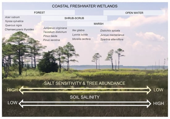
Figure 1.
Plant communities in coastal, non-tidal freshwater wetlands are comprised of salt-sensitive forest, shrub–scrub, and salt-tolerant marsh species. Soil salinization varies in response to heterogeneous microtopography and response to gradients in elevation and vegetation abundance from estuarine waters to tree-dominated wetlands. Coastal tree species that dominate forested wetlands have species-specific sensitivity to salinization and are therefore susceptible to ecosystem transition. Several of these tree species included in this study are deciduous hardwoods (Acer rubrum, Nyssa sylvatica, and Quercus nigra) and evergreen or deciduous conifers (Juniperus virginiana, Taxodium distichum, and Pinus taeda). The background image is a modification of a photograph taken by S. Anderson in Swan Quarter National Wildlife Refuge in North Carolina, USA.
Salinization affects the metabolism of many plant species by disrupting normal physiological function [5,15]. For continued growth and reproduction when exposed to abiotic stressors, plants must adjust physiological processes such as plant water status, photosynthetic activity, and carbon allocation [16]. In long-lived plants, like trees, physiological responses to stressors are often temporary but can significantly affect overall plant performance, hindering growth and the ability to compete for resources in stressful environments for years [17]. Our ability to detect a plant’s stress response is dependent upon the type of environmental stressor, or the combination of stressors, and responses are not always consistent across species, time, and/or space. Plant responses to salt stress are well studied, and changes in plant water status and photosynthetic function are often reliable indicators of changes in function due to stress [5,18]. However, salt sensitivity of some well-studied woody plants (e.g., Taxodium distichum (L.) Rich., Pinus taeda L., and Morella cerifera L.) have been found to be variable across species, geographies, and life-history phases [12,17,18,19,20,21,22,23].
Salinity, drought, and flooding are primary environmental stressors in low-lying coastal ecosystems experiencing climate change (e.g., sea-level rise, saltwater intrusion, and frequent storm events) and anthropogenic impacts on hydrology and nutrient balance [1,24]. Overall, the physiological responses of plants to these stressors are similar in many ways. Salt stress disrupts plant water use, alters leaf pigmentation, and inhibits photosystem II, all of which inhibit photosynthesis [5,25]. When combined with flooding, the negative effects of salinity exposure in terrestrial plants are exacerbated [17,18,20,26]. Many trees exposed to oligohaline and mesohaline conditions (~0.5–8 parts per thousand (ppt)) in the porewater or surface water experience osmotic stress and salt toxicity (i.e., chloride, sodium, sulfate) [12,20,27]. If salt exposure persists, plants undergo photoinhibition and photooxidation [28] similar to the physiological responses during drought [29]. Dissolved salts reduce the osmotic potential of water and can induce water stress in plants, resulting in changes in stomatal conductance, which cause leaf wilting and/or stem embolism [20,30]. In forested wetlands with high tree density, water stress also reduces transpiration [7] and increases greenhouse gas emissions [31]. To prevent irreversible damage to photosynthetic machinery, plants can avoid salt stress by closing stomata to reduce water use or through ionic uptake and/or excretion of salts through photosynthetic leaf tissue [17]. Plant responses to salt exposure are dependent on prior exposure and species-specific levels of plasticity [32]. However, there are limits (thresholds) to a plant’s ability to adjust to stress, which in turn has broader implications for transitions occurring in wetland plant communities [33,34,35].
Salt-stressed plants use light differently. To avoid photoinhibition and photooxidation, chlorophyll molecules in the leaf normally compensate for excess light energy in three different ways: (1) by converting it to photochemical energy via photosynthesis, (2) by releasing it as heat in non-photochemical quenching (NPQ) by photosystem II, or (3) by emitting it as fluorescence [36,37]. Shifts in all three light-use strategies to indicate stress responses in plants have been detected using leaf-level measurements of chlorophyll fluorescence [38]. In combination with analyses of leaf gas exchange and water potential, we can gain detailed insight into how plants metabolize and use water differently under stress. In general, it can be difficult to diagnose what stressors are affecting a plant or an ecosystem, but fortunately, there are non-invasive methods for detecting plant stress at the leaf-level, local, or regional scales [8]. Some of these methods can even target specific stress responses related to leaf photosynthesis, leaf pigmentation, biochemistry, and water content. When combined with controlled mesocosm experiments in the laboratory or greenhouse, we can target specific stressors more easily while controlling the severity of a single stressor. In combination, chlorophyll fluorescence and spectral reflectance indexes have been shown to be reliable indicators of salt stress in coastal tree and shrub species M. cerifera and Baccharis halimifolia L. [39,40].
The goal of this study was to assess the sensitivity of coastal tree species to seawater using multiple different potential indicators of stress. We investigated whole plant performance, productivity, water use, leaf physiology, and leaf fluorescence [41,42,43] in dominant coastal tree species that we would expect to have a range of sensitivities to soil salinity [10] when exposed to pulses of seawater. Salinity treatments were modeled after prior studies by Poulter et al. [20] and Powell et al. [29] and verified by species-specific threshold change points calculated by Anderson et al. [10]. We sought to investigate the relationship between leaf-level physiological changes and leaf spectral reflectance.
The two primary questions that we sought to answer were the following: (1) Which common taxa found in freshwater forested wetlands of the southeastern U.S. are the most and least sensitive to elevated saltwater exposure? And (2) what physiological responses are reliable indicators of plant performance when exposed to moderate pulses of seawater? To address these questions, we conducted a greenhouse experiment to assess the responses of the following contrasting but co-occurring hardwood (Acer rubrum L., Nyssa sylvatica Marshall, Quercus nigra L.) and conifer (Juniperus virginiana L., Pinus taeda L., Taxodium distichum (L.) Rich.) tree species when exposed to a gradient of seawater concentrations.
2. Materials and Methods
2.1. Experimental Approach: Tree Species and Salinity Treatments
We conducted a six-month mesocosm experiment in the greenhouse from May to October 2018 using 118 tree seedlings to investigate plant performance and leaf physiology of common tree species from the coastal plain of the South Atlantic United States when exposed to seawater. Species responses to pulses of seawater were assessed based on the magnitude of change in performance including plant water status, leaf functional traits, leaf gas exchange and fluorescence, and leaf spectral reflectance. Here, we sought to gain a deeper quantitative understanding of tree sensitivity to low, relevant concentrations of soil salinity found in forested freshwater wetlands in eastern North Carolina experiencing episodic pulses of saltwater through surface and groundwater.
This study focused on six species that are common to fresh and brackish wetlands in the coastal plain of North Carolina and throughout the Southeastern U.S.: Acer rubrum (ACRU), Juniperus virginiana (JUVI), Nyssa sylvatica (NYSY), Pinus taeda (PITA), Quercus nigra (QUNI), and Taxodium distichum (TADI). We chose these species to represent a range of natural history strategies (i.e., growth strategy, successional status, leaf longevity, and structure), societal benefits (i.e., economic work/lumber value, wildlife preference, conservation concern), and species occurrence along a natural salinity gradient at field locations throughout the Albemarle-Pamlico Peninsula in eastern North Carolina. In this region, Anderson et al. [10] found soil sodium (the second most dominant ion in seawater after chloride (Cl−)) ranged from 0.1–9.3 ppt, and a salinity threshold for sensitive plant taxa at ~0.3 ppt where a significant portion of species was lost. Five of the six tree species included in this study begin to decrease in their dominance at 0.1–0.3 ppt of sodium (Na+). In addition, we selected several tree taxa based on how frequently they were studied for comparison (e.g., T. distichum, P. taeda) [44,45,46] or paucity of knowledge regarding their salinity tolerance (e.g., A. rubrum, J. virginiana, and Q. nigra) [12,46] and the strategies they employ to cope with salinity stress.
All trees were planted as one-year-old bare root seedlings except N. sylvatica and several Q. nigra individuals, which were germinated from seed in October 2017 (Ernst Conservation Seed Inc., Meadville, PA, USA). All other seedlings were germinated from seed in spring of 2017 from various geographic sources (Mellow Marsh, Siler City, NC, USA, and U.S Forest Service, Raleigh, NC, USA). J. virginiana and N. sylvatica seedlings experienced higher rates of mortality from overwintering in cold chambers prior to propagation; therefore, fewer replicates were included in comparison to the other species (18 and 12 total individuals, respectively). Q. nigra also experienced increased mortality, so several replicates were of younger germinates; however, the same age tree from a different source was tracked throughout the experiment. If a basin was missing a replicate of one of the six species, an additional seed-germinated Q. nigra seedling replaced the missing tree. There were not enough individual N. sylvatica trees to include four intermediate salinity treatments (0.5, 1, 5, and 6 ppt).
In February 2018, all seedlings were planted in standard sterile peat-based media (Fafard® P4 Mix, Sun Gro Horticulture, Agawam, MA, USA) and acclimated in the greenhouse for three months (700 µmol m2 s photosynthetically photon flux density (PPFD) for 16 h per day, 27.8 °C day, and 24.4 °C night temperature and 35% relative humidity). Then, all trees were moved to a larger greenhouse once ambient conditions met those of the prior greenhouse before salinity dosing. Trees were exposed to a salinity gradient with eight treatment concentrations, ranging from controls (no salt added) to 6 ppt simulating fresh (oligohaline) to brackish (mesohaline) conditions found in forested wetland in eastern NC [34,47]. Salinity treatments were dosed with the amount of dissolved Instant Ocean® (Spectrum Brands, Inc., Blacksburg, VA, USA) according to manufacturer’s guidelines in ppt. Instant Ocean® mimics concentrations of salts and micronutrients in seawater, and here, it was used for salinity treatments to be consistent across replicates and decrease the potential for introducing pollutants not relevant to this study. Actual salinity of the stock solution diluted for each treatment level was analyzed to reach target concentrations after the first dose. The two primary treatments (control and 3 ppt) were set up in a randomized complete block design, each with 8 replicates. Individual, non-replicated trees were grown in intermediate (0.5, 1, and 2 ppt) and high (4, 5, and 6 ppt) salinity saltwater concentrations for regression analyses only and not used for inference of statistical results (Figure 2).
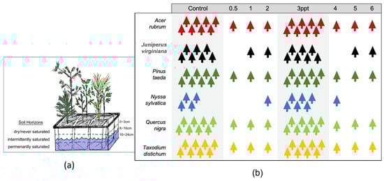
Figure 2.
(a) Conceptual drawing of one basin with one tree of each of the six tree species and the groundwater level (8–16 cm) that was maintained in each of the 22 basins from the greenhouse study. (b) A schematic of the number of replicate trees within each experimental treatment (in parts per thousands; ppt) for each species. The two primary treatments (control and 3 ppt) highlighted in grey ranging from 4–8 replicates per species and individuals for intermediate and high salinity treatments for regression analysis only. All 118 trees were grown in the same greenhouse and the same basin setup.
Salt treatments were administered using a simulated groundwater approach—submerging all tree pots into basins inoculated with stock water collected from Timberlake Observatory Wetland Restoration (TOWeR) site in Alligator, NC (35.898095, −76.167048) [48]. Applying the seawater treatments from belowground allowed us to simulate a realistic delay in salt exposure to living belowground tissue via groundwater pathways. All six tree species were grown in each salinity treatment-specific basin (i.e., block). Before treatments were introduced, water chemistry (pH, DOC, ortho-P, NH4, anions, and cations) was measured on the stock water used as the solvent for each treatment, and reverse osmosis (RO) water was tested for salts prior to use for water replacement in the basins throughout the experiment.
To isolate the influence of salinity on tree physiology, we applied two pulses of seawater and maintained constant root inundation throughout the entire experiment. The first saltwater pulse was applied on 1 May 2018, after trees had established roots and have begun to leaf out (~12 weeks). A second pulse was dosed on 15 August 2018, once saltwater concentrations in the groundwater of salt-treated basins from the first dose were diluted and no longer different across treatments. Water depth in each basin was monitored biweekly to maintain three moisture horizons below the soil surface: dry/unflooded (0–8 cm), intermittent saturated (8–16 cm), and permanently saturated (16–24 cm) (Figure 2). We chose moisture horizons to reflect the annual average water-table depth in research plots at the TOWeR site where we have monitored groundwater levels continuously throughout 2017 and 2018. Our aim was that soils in the upper horizon (0–8 cm) remained permanently dry, the lower horizon (16–24 cm) remained permanently saturated, and the intermittent zone was allowed to dry before rewetting. Any water loss via transpiration and/or evaporation was replaced by adding RO water directly to the treatment basin up to the top of the intermittent horizon (8 cm from the soil surface).
Ambient greenhouse conditions (27.1 +/− 7.23 °C, 80.0 +/− 9.82% relative humidity, 152 +/− 291 PAR) were monitored continuously using in-house sensors (Duke Phytotron) and two temperature/light sensors (Onset Computer Corp. Hobo Pendant®, Bourne, MA, USA) placed in the greenhouse. Shortly after dosing salt treatments (15 May 2018), 250 g of sterilized leaf mulch was added to the soil surface of each pot to reduce soil surface drying. Starting on June 12, 200 mL of fertilizer (half-strength Hoagland’s solution) was added to the soil surface of each pot every two weeks throughout the entire experiment to reduce nutrient limitation in the soil. Soil temperature and soil moisture were monitored weekly at 12 cm depth from the soil surface (Campbell Scientific HydroSense II with CS655 sensor, Logan, UT, USA).
Conductivity, temperature, and pH of the groundwater in each basin were monitored biweekly using a multi-parameter water sensor (YSI Professional Plus (Yellow Springs, OH, USA) or Eureka Manta2 (Austin, TX, USA)) including before and after water was added to a basin to ensure consistent water chemistry after additions. Monthly water samples were collected from each of the 22 basins, filtered (glass-fiber filters 0.7 μm), and frozen for additional water chemistry analysis. Analyses of anions (Cl−, SO4−, NO3−) and cations (Na+, Ca+, Mg+, K+) were run on a Dionex ICS 2000 (Dionex Corporation, Sunnyvale, CA, USA), nutrients (NH4+, PO4−) on a Lachat QuickChem 8500 (Lachat Instruments, Loveland, CO, USA), and total nitrogen (TN) and dissolved organic carbon (DOC) on a AS-18 analytical column and Shimadzu TOC-VCPH Analyzer with TNM-1 module and ASI-V autosampler.
Soil conductivity was measured in each individual pot at 5 cm and 10 cm depths using a soil probe (Hanna HI98331 Soil Test™, Woonsocket, RI, USA) pre-calibrated to salinity tested in the field. Soil conductivity was intensively measured every other day during the first 2 weeks and once a week thereafter to identify when plant roots in the upper top 10 cm were fully exposed to the salinity treatments. During the final harvest, soil conductivity was measured three times at each of the three soil depths using the same probe. We also collected bulk soil subsamples composited from all three horizons to measure soil properties and water-extractable chemistry, including % soil moisture, organic matter content, pH (Mettler Toledo DL18 titrator pH probe, Columbus, OH, USA), and anions (Cl−, SO4−, PO4−, NO3−) and cations (NH4+, Na+, Ca+, Mg+, K+) on a Dionex ICS 2000, and Lachat QuickChem 8500.
2.2. Functional Traits, Leaf Loss, and Biomass
We quantified performance by evaluating aboveground biomass by plant compartment, growth rate, total leaf area, leaf litter fall, multiple leaf functional traits, and belowground biomass by depth and flooding frequency. Functional traits included specific leaf area (SLA), leaf dry matter content (LDMC), and leaf carbon and nitrogen concentrations. Leaf litter was collected whenever fallen leaves were observed or weekly from 19 July, when substantial leaf litter began to accumulate, until 17 October. Leaf litter was dried at 65 °C for a minimum of 72 h and weighted. Mass of leaf litter loss was assessed over time and summed to calculate proportion of leaves lost (relative to the whole-plant leaf mass) and rate of leaf loss (mg leaf dry matter per day). During final harvest, we measured the dead P. taeda leaves (void of chlorophyll) separate from healthy/green leaves since leaves on the terminal branch generally did not drop.
We destructively harvested above- and belowground biomass at the conclusion of the experiment (17–19 October 2018) to assess total productivity for each tree. All replicate trees of each species were processed in a single day. Seedling height and diameter were measured monthly to assess relative growth over the course of the experiment. Height was a measure of each individual tree from the soil surface to the highest photosynthetically active materials and diameter at soil surface/root collar [49]. Biomass was compartmentalized into leaf (excluding petiole), stem, and root mass to calculate total biomass, root-to-shoot ratio and root mass fraction, and total root mass at each of the three soil horizons (i.e., dry, intermittent saturated, and permanently saturated) (Figure 2). All biomass was dried for a minimum of 72 h at 65 °C before weighing. Relative growth rate (RGR) for each tree was calculated as the following:
where the difference in tree height of post-treatment (Hpost) and pre-treatment (Hpre) represent biomass allocation over the 6 months of the experiment [20]. Stem diameter (Dpost and Dpre) was calculated in the same way.
(Hpost − Hpre)/Hpre,
2.3. Osmotic and Leaf Water Potential
Prior to harvesting all plant biomass at the end of the experiment, we measured leaf water potential (ΨL in units of mPa) in three fresh leaves of each treatment per species (18 total leaves) at predawn (Ψpd) from 05:20–07:10 across two consecutive days using a pressure chamber (PMS Instruments, Albany, OR, USA). We collected an additional leaf from each tree to measure midday leaf water potential (Ψmd) from 12:00–14:00 to test the difference in plant water status between Ψmd. and Ψpd of each species in response to the gradient of saltwater exposures. Leaves were selected from the upper portion of the tree between the 3rd and 6th leaf position down from the terminal end of the apical meristem [50] to capture mature new growth. Single leaves of J. virginiana and P. taeda were too small to be measured in the pressure chamber, so we measured ΨL on terminal branch segments that had not become woody and were comparable in size to leaf samples from other species. Leaves were later dried, weighted, and tallied with total leaf biomass of each tree.
Additionally, we measured osmotic potential (Ψπ in mPa) of groundwater after dosing saltwater in the groundwater of each treatment basin. We used groundwater concentrations of NaCl (mg/L) two hours after the second dosing on August 15 to calculate Ψπ using the Van’t Hoff equation:
where i is 2 (for NaCl), C is concentration of NaCl in molarity, R is gas constant (8.32 × 10⁻³ MPa L mol−1), and T is temperature in Kelvin. Treatment-specific Ψπ was compared to Ψpd, which is a proxy for soil water potential [51] to assess species-specific responses to the expected osmotic potential of the solute concentrations. From this, we estimated the position along the salinity gradient that each species reached equilibrium (Ψπ − Ψpd = 0). Equilibrium is the point where water would stop flowing from the soil into the roots, in this case, driven by increasing Ψπ, or soil salinity high on the gradient. It is beyond this point where we would expect salinity stress to have major implications on plant function, behaving much like drought during low water supply to the roots.
Ψπ = −iCRT,
2.4. Leaf Gas Exchange, Chlorophyll Fluorescence, and Spectral Reflectance
Once a month, leaf photosynthesis (Anet μmol CO2 m−2 s−1), stomatal conductance to H2O vapor (gwv mol H2O m−2 s−1), and chlorophyll fluorescence were measured simultaneously using an open gas exchange system (Li-Cor 6400; Li-Cor Biosciences, Lincoln, NE, USA) mounted with a pulse-amplitude modulated fluorometer chamber (Li-Cor 6400-40). One mature sun leaf (5–7 leaves down from the terminal end) was selected per tree (a different leaf each month) with parameters of light intensity set to 700 µmol m−2 s−1, block temperature 25 °C, and sample CO2 at 400 µmol m−2 s−1 following the setup procedure used by [52]. Once the sample chamber reached equilibrium, five evenly spaced samples were logged for each leaf and averaged for analysis. Sample relative humidity in the chamber was maintained at ambient concentrations (mean = 61%, s.d. = 10.4%). If desiccant scrubber was not able to regulate chamber humidity to expected levels, sampling was discontinued, and desiccant was changed before next use.
We measured carbon-13 (13C) isotopes in leaves of four of the six tree species (A. rubrum, J. virginiana, P. taeda, and T. distichum) as a measure of intrinsic water-use efficiency (δ13C) to assess if leaves exposed to increased salinity of 3 ppt were discriminating against the lighter carbon isotope, 12C, due to stomatal closure with increase salt stress [53]. Of the five leaves used to measure leaf functional traits, three were ground and analyzed for carbon isotope 13C on a Carlo Erba NA 1500 Elemental Analyzer (Thermo Scientific, Waltham, MA, USA), fitted with a Costech zero-blank autosampler (Duke Environmental Stable Isotope Laboratory, Durham, NC, USA). The methodology we used for sample collection and processing of all traits listed above follows Pérez-Harguindeguy et al. [49].
Fluorescence measurements were taken on light-adapted leaves across all species and treatments simultaneously with gas exchange. Three randomly selected leaves from three individual trees were selected per species for fluorescence of dark-adapted leaves for a minimum of 30 min using dark-adapting leaf clips (LI-COR Biosciences, Lincoln, NE, USA). We used light-adapted leaf fluorescence measurements to calculate operating efficiency of PSII photochemistry (ΦPSII) in light-adapted leaves, which measures a proportion of absorbed light used in PSII photochemistry [36,37,38] and used as an indicator of salinity stress [27,43]. ΦPSII is calculated as
where F’m is the maximum fluorescence following a light pulse in a light-adapted leaf, and F’ is the steady-state fluorescence of that leaf after a waiting period when fluorescence can reach equilibrium again.
ΦPSII = F’m − F’/F’m,
We measured leaf reflectance in the visible and near-infrared spectrum (400–1100 nm) monthly using a spectroradiometer (Apogee PS-100, Apogee Instruments Inc., Logan, UT, USA) across species and all eight salinity treatments. After calibrating the spectroradiometer to a white and black standard (Apogee AS-004), a fixed light source was held at 45° from the leaf/leaves surface with a reflectance probe (Apogee AS-003, Apogee Instruments Inc.). We measured the leaf reflectance of five leaves per individual tree by logging ten measurements per leaf every three seconds. Later, we generated a reflectance curve by averaging the five leaves per tree and then across salinity treatment. We extracted wave lengths from the reflectance data in R [54] to calculate normalized difference vegetation index (NDVI) [55] and photochemical reflectance index (PRI) [56]:
where each number is a wavelength in nanometers (nm). We also assessed the entire wavelength profile to visually inspect the sensitivity of each curve to changes in soil salinity. We merged reflectance data profiles generated in the Apogee software using the Specalyzer web application and in apogeereader package [57] in R [54].
NDVI = (800 − 680)/(800 + 680), and
PRI = (570 − 531)/(570 + 531),
2.5. Statistical Analysis
We analyzed all soils and water chemistry parameters as response variables in generalized linear mixed-effect models (glmer) with the lme4 package [58] in R [54] to determine the differences in salinity treatments across all species over time and their interactions. We included basin (each containing all tree species of like salinity treatment) number in the model as a random effect to reduce the influence of basin position in the greenhouse. Generalized linear models (glm) and two-way analysis of variance (ANOVA) with Tukey’s test for mean separation were used to test the significance of the effects of salinity treatment and species on soil nutrients (NO3−, NH4+, and PO4−). Since much of these data were continuous, non-negative, and right-skewed, we used gamma or Gaussian family distributions and compared models with log and identity links using Akaike’s information criteria (AIC). We also used lsmeans as a post-hoc test of the significance of contrasts between each salinity treatment (p ≤ 0.05). All statistics were performed in R [54].
Additionally, we used generalized linear models with an analysis of variance (ANOVA) to test the variation in mean effects of functional traits within and across all salinity treatments for each of the six tree species included in the experiment. Two-way ANOVA (using Bonferroni correction) was used to test for differences (p < 0.05) in leaf traits (e.g., SLA, LDMC) across species and salinity treatments as measured at final harvest. Leaf litter data were analyzed using glmer to test for differences across species and salinity treatments and their interactions over time. Again, we used AIC in all our analyses to compare models using gamma family, log and identity links, and lsmeans to conduct a post-hoc test with Tukey’s adjustment to test significance of contrasts between controls and each salinity treatment. Effect sizes between mean treatments (control and 3 ppt) were calculated using Hedge’s g using cohen.d in effsize package, and effect sizes were categorized as small (|g| < 0.5), medium (|g| = 0.5–0.8), or large (|g| > 0.8) effect sizes. All data visualizations were generated using the ggplot2 [59] package in R Studio [60].
3. Results
3.1. Groundwater and Soil Chemistry
We achieved significant separation of salinity across each replicated treatment (controls and 3 ppt) shown by measures of specific conductance and ion concentrations in groundwater (Figure 3 and Table A1). Aside from periodic overlap between low (0.5–2 ppt) and high (4–6 ppt) non-replicated treatments (e.g., early June and mid-September), the two peaks (~9000–10,000 μs/cm) in conductivity were the days when the salt stock was dosed, with a gradual decline from May 1–August 15 in groundwater salinity following each dosing event (Figure 3). Overall, groundwater temperature and pH (22.4–29.9 °C and 6.0–7.5, respectively) were relatively constant across treatments throughout the course of this experiment with some increase and decrease spikes in all treatments likely due to instrument calibration. The groundwater in the control basins at the end of this experiment (10 October 2018) had PO4+ concentrations of 0.75 +/− 0.09 mg/L in the control basins and 0.70 +/− 0.18 mg/L in the 3 ppt basins. Ammonium (NH4+) concentrations were <0.01 mg/L in both the control and 3 ppt treatment basins.
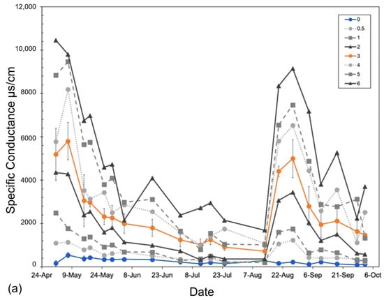
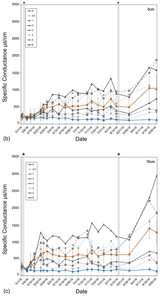
Figure 3.
Specific conductance (µs/cm) of (a) basin groundwater and (b,c) tree pot soils measured from 1 May to 26 September 2018, averaged across all experimental basins within each treatment over the entire 6-month experiment. Soil-specific conductance measured at (b) 5 cm and (c) 10 cm depths from the soil surface. The two replicated treatments are in color: control (green) and orange (3 ppt). All other intermediate (0.5, 1, and 2 ppt) and high (4, 5, and 6 ppt) treatments are in a gradient of grey circles and dotted lines (0.5 and 4 ppt), squares and dashed lines (1 and 5 ppt), or triangles and solid lines (2 and 6 ppt). Non-replicated intermediate treatments (in grey) are shown to highlight trends only. Error bars are the standard deviation for both replicated treatments (control and 3 ppt). The vertical shaded bars in the soil conductance (b,c) noted by the asterisks above the figure indicate salt additions, or pulses, added to the groundwater of each treatment basin.
Soil conductivity increased faster at a 10 cm depth than at a 5 cm depth (Figure 3). Soils reached maximum salinity after ~21 days at 10 cm, while it took approximately three times as many days (after the second salinity pulse) for soils at 5 cm to reach comparable levels (Figure 3). Soil salinity was consistently higher at 10 cm than at 5 cm. Regardless of sampling depth, salinity increased continuously throughout the entire experiment, not showing any signs of two pulse additions dosed to the groundwater (Figure 3). Soil temperature was largely consistent across all treatments but varied week to week as the basin positions within the greenhouse were randomized weekly. Soil moisture was also largely consistent across treatments except that the 0.5 ppt and 6 ppt treatments tended to have a higher soil moisture than all other treatments on 1 May and 30 July, respectively.
Soils from each pot were mixed, subsampled, and analyzed for % soil moisture, organic matter content, pH, and anions (Cl−, SO4−, PO4−, NO3−) and cations (NH4+, Na+, Ca+, Mg+, K+), shown in Table A2. Interestingly, maximum soil salinity was greater (p < 0.01) in conifers (max = 0.66–0.79 μg Na+ g−1) compared to hardwoods (max = 0.42–0.59 μg Na+ g−1) (Table 1). All environmental variables unrelated to salinity treatment (% soil moisture, organic matter content, pH) were not different across treatments. The only unexpected difference across treatments was that the 5 ppt treatment had lower mean salt concentrations compared to the 4 ppt treatment. The 0.5 ppt treatment also had lower concentrations of SO4−, Ca+, Mg+, and K+ compared to the control. These results are also reflected in the soil conductivity measured at various times throughout the experiment (Figure 3).

Table 1.
Soil salinity broken down by species. Chloride (Cl−) and sodium (Na+) concentrations are in bold and highlighted grey to show the elevated concentrations in the conifers compared to the hardwood species. Additional soil salinity statistics are reported in Table A2.
We analyzed water-extractable soil nutrient concentrations (PO4−, NO3−, and NH4+ g per g soil) across all species binned (control, low, mid, and high) salinity treatments. Soil NH4+ increased in soils with 4–6 ppt salinity (p < 0.001), and soil NO3− increased when exposed to 3 ppt salinity but not at higher concentrations (p = 0.007) (Figure A1). Interestingly, we found an interaction between species and treatment on NH4+ and NO3− (p = <0.001). That is, NH4+ and NO3− concentrations were dependent on what species was growing in the soil. NH4+ increased with 3–6 ppt salinity in Q. nigra and T. distchum (p = <0.006) and with 4–6 ppt salinity in A. rubrum and P. taeda pots (p < 0.007). Soil NO3− increased in the presence of T. distchum in trees exposed to 3 ppt salinity (p = 0.0001). We found soil NH4+ and NO3− concentrations in soils exposed to high salinity (4–6 ppt) decreased in J. virginiana soils (p = 0.04 and 0.001, respectively). N. sylvatica soil NH4+ and NO3− did not have a consistent pattern related to increased salinity; however, increased replication for high salinity concentrations would likely result in a similar outcome to all other increasing species since the effect was marginally significant (p = 0.08).
3.2. Functional Traits, Leaf Loss, and Biomass
Total whole-plant leaf area (LA) decreased in A. rubrum (p = 0.02) and tended to increase in P. taeda (p = 0.06) trees exposed to salinity 4–6 ppt (Figure A2). However, when assessing leaf area by absolute soil Na+ concentrations, we found a negative relationship between species and soil Na+ in A. rubrum and P. taeda (R2 = 0.40 and 0.17, and p = 0.04 and 0.05, respectively). A. rubrum also experienced a significant amount of leaf loss when exposed to 3 ppt (p = 0.037) and 4–6 ppt (p = 0.041) salinity treatments (Figure A3). Leaf loss in A. rubrum was also dependent on the interaction of time and salinity treatment. Acer rubrum trees in high salinity treatments (4–6 ppt) did not lose a large proportion of leaf mass until after the second saltwater pulse (15 August 2018).
Taxodium distichum trees exposed to 4–5 ppt did not experience a significant increase in leaf loss; however, the individuals exposed to 6 ppt salinity experienced a significant amount of leaf loss toward the end of the experiment. In addition, P. taeda experienced mixed responses in leaf loss and increased (p = 0.009) and decreased (p = 0.007) in 3 ppt and 4–6 ppt salinity exposure, respectively. However, it is important to note that P. taeda only lost ~2%–8% of total leaf mass. We observed a significant amount of leaf discoloration and death in salt-exposed P. taeda trees, but many of these leaves were not lost as litter and therefore not collected as litter loss. Dead leaves represented 6.6%–49.5% of total leaves in salinity treatments from trees exposed to 3 ppt and 6 ppt salinity treatments.
Untreated evergreen trees (J. virginiana and P. taeda) had different specific leaf area (SLA) compared to the deciduous species, and A. rubrum and Q. nigra had similar SLA, while N. sylvatica and T. distichum had different SLA (Figure A4). When comparing seawater-treated trees to controls, A. rubrum and T. distichum SLA increased in mid- and high-salinity treatments (p = ≤0.01). N. sylvatica leaves also increased with 4–6 ppt salinity compared to low (3 ppt) salinity exposure (p = 0.049; p = 0.054 compared to controls). J. virginiana was the only species that decreased in SLA (i.e., leaves became smaller and/or thicker) when trees were exposed to ≥3 ppt salinity compared to 0.5–2 ppt exposed trees (p = 0.046). A. rubrum, J. virginiana, Q. nigra, and T. distichum all had unique leaf dry matter content (LDMC mg g−1 (mg dry leaf mass per g water-saturated fresh leaf mass), p = < 0.0001–0.046,), while N. sylvatica and P. taeda had comparable LDMC. A. rubrum and T. distichum trees exposed to 3–6 ppt and 4–6 ppt salinity increased their LDMC (p = 0.0002–0.0054, and p = 0.0004 respectively). Conversely, the LDMC in Q. nigra decreased with salinity for the 4–6 ppt treatment (p = 0.048).
Leaf percent carbon and nitrogen content varied by species (A. rubrum, J. virginiana, P. taeda, and T. distichum) and salinity treatment (control and 3 ppt). Percent leaf carbon decreased while nitrogen increased in A. rubrum (p = <0.001 and 0.009), and nitrogen increased in T. distichum when exposed to 3 ppt salinity (p = 0.003). P. taeda had the lowest nitrogen content across all four species, but neither leaf carbon nor nitrogen content changed with increased salt exposure.
Differences between the control and 3 ppt treatments for biomass, growth, and functional trait responses are shown as effect sizes (Figure 4) and actual mean values (Table A3). Of the twelve performance parameters we measured in this study, A. rubrum showed seven mean decreases (BGB, LM, LA, DGR, RSR, leaf %C, and C:N) and two increases (leaf %N and SLA) in 3 ppt salinity treated plants compared the controls. T. distichum also had a mean increase in leaf %N and a mean decrease in leaf C:N like A. rubrum.
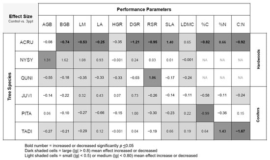
Figure 4.
Summary table of effect sizes (Hedge’s g) between control and 3 ppt salinity treatments for plant performance parameters including leaf mass and area (LM and LA), specific leaf area (SLA), leaf dry matter content (LDMC), leaf percent carbon and nitrogen (%C and %N), leaf carbon–nitrogen ratio (C:N), aboveground biomass (AGB), belowground biomass (BGB), height and diameter growth rates (HGR and DGR), and root-to-shoot ratio/root mass fraction (RSR). Dark-shaded cells indicate a large mean increase or decrease in effect sizes compared to controls. Light-shaded cells indicate a small or medium effect size compared to control. If differences in means were significant (p ≤ 0.05), values are bold. White cells indicate no difference.
3.3. Osmotic and Leaf Water Potential
We found significant effects of species (F = 11.6 and, p = <0.001) and salinity treatment (F = 5.4, p = <0.001) on predawn water potential (Ψpd). Leaf Ψpd in A. rubrum was less negative than Q. nigra, J. virginiana, and P. taeda (p = <0.03). Both A. rubrum and T. distichum were closest to equilibrium (Ψπ − Ψpd = 0) and gradually declined toward zero as salinity treatment and Ψπ increased (Figure 5 and Figure A5). Conversely, J. virginiana leaf Ψpd was more negative than A. rubrum and T. distichum (p < 0.021) and did not change at any salinity/solute osmotic potential. Overall, with salinity exposure < 6 ppt, Ψpd increased, and Ψπ decreased with increased salinity; however, water transport was maintained in all species except for P. taeda, where equilibrium was reached at Ψπ −0.35 MPa. This is where water ceases to move from the soil into the roots (Figure 5). Hardwoods did not reach equilibrium, and Ψπ was never less negative than Ψpd.
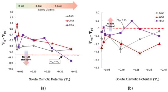
Figure 5.
(a) The relationship between osmotic potential (Ψπ, MPa) of the groundwater treatment solutions (NaCl) after the second salinity dose and the difference between Ψπ and predawn leaf water potential (Ψpd, MPa) across all species and salinity treatments. Each color and shape combination represents Ψπ and Ψpd for each species. The horizontal arrow (color gradient from green to red) represents the direction of salinity increase as Ψπ becomes more negative. The vertical arrow in the panel shows that as Ψpd decreases in tandem with a decrease in Ψπ, hydrological flow between the soil and roots reaches equilibrium and ceases to move resulting in leaf loss and mortality. The points closest to zero on the x-axis are controls, and salinity treatments increase as they move to the right (more negative Ψπ) noted by the green-to-red gradient arrow. (b) The relationship between osmotic potential (Ψπ) of the groundwater treatment solutions (NaCl) and the difference between midday water potential (Ψmd) and Ψpd across all species and salinity treatments. As Ψπ increases (salinity treatments become more saline), hydrological flow between the soil (Ψpd) and light-adapted leaves (Ψmd) reach equilibrium (Ψmd − Ψpd = 0; noted by “No H2O Transport”). Equilibrium is expected at high soil salinity meaning water would cease to move to more negative pressure potential in the leaves.
Midday leaf water potential (Ψmd) was different across species (F = 18.4, p = < 0.001) but not statistically affected by salinity (F = 0.674, p = 0.724). The difference between midday and predawn potential (Ψmd − Ψpd) was also different across species (F = 13.54, p = < 0.001) but not affected by salinity. Interestingly, P. taeda treated with 4 ppt salinity (Figure 5) did cross zero/equilibrium (Ψmd = Ψpd, i.e., Ψmd − Ψpd = 0 MPa) around Ψπ = −0.2 MPa Ψπ where we expect water transport would stop midday due to salinity or drought since Ψpd was quite low at around −0.8 MPa. However, diurnal water transport continued in all other treatments.
3.4. Leaf Gas Exchange and Chlorophyll Fluorescence
There was an interaction between the species and grouped salinity treatment for photosynthesis (Anet) rate (p = 0.013); however, when we tested the main effects of species and salinity treatment (control and 3 ppt), species was a significant predictor of photosynthesis over time (p = <0.001), but salinity was not (p = 0.75). We found that each species’ responses differed among salinity treatments. A. rubrum, T. distichum, and N. sylvatica all had decreases in the mean photosynthesis rate in the salinity treatments compared to the controls as the experiment progressed (Figure A6). A. rubrum photosynthesis decreased when exposed to 3 ppt (p = 0.005) and marginally to 4–6 ppt salinity in October (p = 0.083) and July (p = 0.08). N. sylvatica photosynthesis decreased in August when exposed to 3 ppt salinity (p = 0.008), as did T. distichum in September, but in low salinity (0.5–2 ppt) (p = 0.03).
We did not find any decreases in stomatal conductance to H2O vapor (gwv) across all species exposed to 0.5–6 ppt salinity exposure (Figure A7). However, we did find an increase in gw in the T. distichum exposed to 4–6 ppt salinity in September (p = 0.04) and 3 ppt salinity in October (p = 0.016). Additionally, we observed a marginal increase in A. rubrum exposed to 3–6 ppt salinity (p = 0.07–0.08). We compared the linear relationship between δ13C (the difference between 13C and 12C ratios between a sample and a standard) and Ci/Ca (the ratio of internal leaf CO2 and ambient CO2 in the air) to detect increased enrichment in the leaves of plants exposed to 3 ppt salinity. We found no significant linear relationships across treatment within all four species tested (A. rubrum, J. virginiana, P. taeda, and T. distichum).
Like photosynthesis, we found a significant interaction between salinity and month on the operating efficiency (in light-adapted leaves) of photosystem II (ΦPSII) (p = <0.001). However, the response of ΦPSII to salinity was not consistent across all species compared to photosynthesis (Figure A8). In July, ΦPSII in A. rubrum decreased when the trees were exposed to 3 ppt salinity and again in August and October in salinity 3–6 ppt; however, these decreases were marginally significant (p = 0.05–0.09). Anet and gwv are highly correlated with leaf physiological processes in terrestrial plants. We found a moderate yet highly significant correlation between Anet and gwv across all species, salinity treatments, and sample dates throughout this study (R2 = 0.52, p = <0.001) (Figure A9). However, when testing the correlation of Anet and gwv in the control and 3 ppt treatments of A. rubrum alone, the relationship in controls (R2 = 0.81, p = <0.001) had a remarkably consistent yet stronger linear relationship compared to the trajectory across species and treatments. Although the linear trends in A. rubrum exposed to 3 ppt salinity were less strong (R2 = 0.59, p = <0.001), and the slope of the linear relationship between Anet and gwv only increased slightly (m = 67.5) compared to the controls (m = 67.1); however, these relationships were not specifically tested. However, the y-intercept decreased as the salt-exposed plants began to decrease photosynthesis but not in gwv.
3.5. Spectral Reflectance
The reflectance spectra in A. rubrum match the expected curvature across the entire visible spectrum, visibly changing slope with increased salinity (Figure 6). We found an interaction between species, salinity treatment, and month (June, September, and October 2018) on PRI and NDVI (p = <0.001) (Figure A10). The PRI decreased in 3, 4, and 6 ppt salinity-exposed trees in June (−0.025, 0.004, and −0.011 respectively), September (−0.076, −0.127, and −0.141), and October (−0.080, −0.080, and −0.149) (p = 0.001–0.04). We also found that NDVI decreased in A. rubrum leaves when exposed to 3, 4, and 6 ppt salinity in September (0.69, 0.41, and 0.45, respectively) and October (0.67, 0.51, and 0.38) (p = <0.001) but not in June (0.84, 0.84, and 0.82). When testing the relationship between PRI and ΦPSII, a non-linear exponential relationship emerged after the second salinity dose in September (F = 7.1, p = 0.015) and became more significant and reflected the salinity gradient treatments more closely in October (F = 8.54, p = 0.009) when compared to June. The NDVI showed the same pattern as PRI.
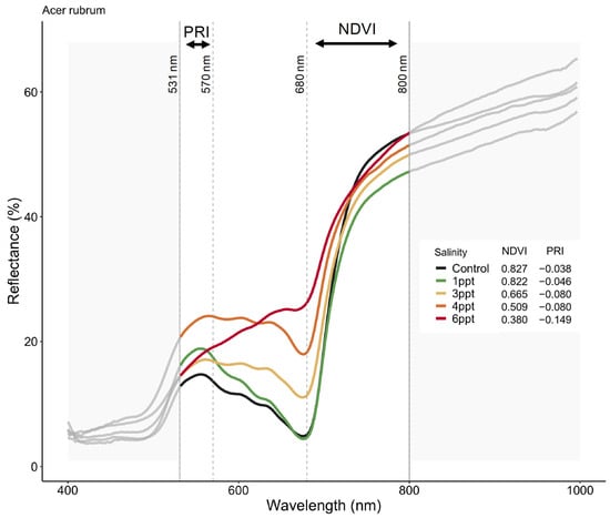
Figure 6.
Reflectance spectra from Acer rubrum leaves in October 2018 for select salinity treatments (control = dark green, 1 ppt = light green, 3 ppt = yellow, 4 ppt = orange, 6 ppt = red) showing the wavelengths expected to correlate with salinity and drought stress (531, 570, 680, and 800 nanometers). Photochemical reflectance index (PRI) is derived from narrowband reflectance at 531 and 570 nanometers (nm), and normalized difference vegetation index (NDVI) derived from red and near-infrared calculated as NDVI = (NIR − Red)/(NIR + Red), which is reflected over the incoming radiation. Here, we used the reflectance values at 680 (red) and 800 nm (infrared) to calculated NDVI. An NDVI close to 0–0.1 corresponds to no vegetation, while NDVI close to 0.8–0.9, as seen here in the control treatment (NDVI = 0.827), indicates the highest possible density of green leaves.
4. Discussion
This study sought to deepen our understanding of tree species-specific sensitivities to low levels of episodic seawater exposure to improve predictions of non-tidal coastal wetland change at broader scales. We have documented the physiological sensitivity of six tree species to oligohaline and mesohaline (0.5–6 ppt) salinity by evaluating the relationships between various measures of plant physiological responses including leaf water potential, gas exchange, chlorophyll fluorescence, and spectral reflectance. We found that A. rubrum was the most sensitive, and J. virginiana the most tolerant species to moderate levels of soil salinity after two exposures of seawater. Juniperus virginiana trees did not display any responses to ≤6 ppt salinity in ΨL, photosynthesis, or chlorophyll fluorescence making it a particularly tolerant species to pulses of salt exposure. J. virginiana is known to be drought and salt-tolerant in a variety of landscapes but is not particularly flood-tolerant [12]. Additionally, there is a subspecies Juniperus virginana var. silicicola (Small) E. Murray, commonly found in sand dunes, marshes, and forests of the Southeastern U.S., and is likely to be even more salt tolerant than J. virginiana var. virginiana [61].
Conversely, A. rubrum, was particularly sensitive to salinity. A. rubrum Ψmd was not significantly impacted by moderate increases in salinity; however, we found no evidence of a reduction in Ψpd in treatments other than the non-replicated tree exposed to 6 ppt salinity and, therefore, maintained water uptake from soil into the roots. Yet, we found that the A. rubrum tree’s leaf functional traits and biomass allocated were impacted more than any other species when exposed to 3 ppt salinity (Figure 4). In addition, A. rubrum photosynthesis decreased after two pulses of seawater at 3–6 ppt within four months of exposure. A. rubrum photosynthesis declined in September and October which coincided with leaf wilt and early leaf senescence in 3–6 ppt salinity treatments. In contrast to J. virginiana, A. rubrum is tolerant to flooding but more sensitive to salt and flooding in combination [62]. Therefore, J. virginiana and A. rubrum may be good indicator species of saltwater stress in freshwater forested wetlands, which reflects what is observed in the coastal plain of North Carolina on the Albemarle-Pamlico Peninsula [10,34]. J. virginiana is often the last tree species scattered throughout non-tidal freshwater and brackish marshes, and A. rubrum trees are not abundant in forested wetlands transitioning to marsh or open water, and seedlings and saplings struggle to survive.
4.1. Salinity Treatments
Our efforts to initiate salinity treatments representative of the targeted saltwater exposure levels, based on the groundwater and soil chemistry, were successful. Even though trees were only dosed with two pulses of saltwater stock, soil conductivity continued to increase throughout the entire experiment, as water lost (via transpiration or evaporation) was replaced with fresh reverse osmosis water (Figure 3).
The goal of our study was to assess the prolonged impacts of salinity pulses. Prior experiments [18] have dosed plants with chronic additions of targeted salt concentrations throughout entire experiments that can quickly accumulate on the soil surface, therefore resulting in reduced growth and physiological activity within 35 days, causing higher mortality rates. This sort of approach causes an accumulation of seawater-derived salts in the soil. In a study conducted by Poulter et al. [20], salt addition of 4 and 8 ppt of P. taeda and Pinus serotina Michx. sapling resulted in complete mortality over 2.5 months. And similarly, Naumann et al. [27] exposed M. cerifera to chronic seawater treatments at 5, 10, and 15 ppt. Salinity exposure at these levels resulted in a rapid (~3–9 days) decline in plant growth and performance at 5 ppt, the complete die-off of leaves, and eventually mortality >10 ppt. Our study highlights the importance of dosing strategy (both concentrations and treatment pathway) when conducting environmentally controlled salinity stress experiments in mesocosms. Additionally, treatments need to be tailored to the species being studied since the maximum soil salinity was greater in conifers compared to hardwoods (Table 1). This result could indicate reduced plant water use in hardwoods, which would dilute available salts in the soil. Alternatively, conifers are more successful at excluding salts from being taken up through the roots [7].
Salt stress in the context of coastal freshwater wetlands is largely an episodic event resulting from storms, droughts, or human disturbance [1]. Although the experimental design is ecologically relevant, we assumed that the susceptibility of earlier growth stages of trees to salinity stress is higher and does not necessarily directly relate to mature trees in situ. However, using seedlings to quantify tree salinity sensitivity is more critical than mature individuals because if young fail to survive salt-stressed conditions, we would not expect recruitment of juvenile trees in forests, resulting in long-term changes in coastal forested wetlands [11].
4.2. Leaf Water Potential, Gas Exchange, Fluorescence, and Senescence
Typically, salinity causes a drop in photosynthesis in salt-sensitive plant species, reducing osmotic potential and stomatal conductance [20]. In our study, P. taeda was the only species where Ψpd increased (nearing equilibrium with Ψπ or Ψmd) when exposed to 5–6 ppt salinity. Therefore, water transport was maintained in A. rubrum, J. virginiana, N. sylvatica, Q. nigra, and T. distichum when exposed to salinity <6 ppt. However, the A. rubrum tree treated with 6 ppt salinity had already lost all its leaves by the time we measured ΨL. We cannot be certain when A. rubrum crossed equilibrium, but our data suggest that A. rubrum is sensitive to salinity >4 ppt since multiple trees exposed to 3 ppt had significant leaf loss. Pinus taeda ΨL tended to reach equilibrium (Ψπ = Ψpd) when water transport of all other species was maintained (Figure 5). Interestingly, P. taeda also reduced the whole-plant leaf area with increased salinity, so we may expect P. taeda growth to suffer in years following saltwater pulse events due to lack of water transport and loss of photosynthetic capacity [18].
Although juvenile trees tend to be more sensitive to salinity and less variable in their tolerance to salinity, their sensitivity is a characteristic ideal for studying plant responses to low concentrations (≤6 ppt) of soil salinity [17,63]. We expected more negative impacts of increased salinity treatments on the photosynthesis rate (Anet) in the six species we tested in this study. Yet, we found A. rubrum to have the most instances of decreased photosynthesis, which coincided with the second salinity pulse. It is not surprising that A. rubrum is the most sensitive to salinity [62]; however, few studies have investigated how A. rubrum, a species known for its wide distribution, responds to multiple pulses of low concentrations of seawater that accumulate in coastal soils.
Trees exposed to low to moderate levels of salinity stress (<6 ppt) leave stomata open when access to freshwater is abundant to allow the plant to continue photosynthesizing under stress; however, increased salinity causes leaf wilt and necrosis, which leads to premature senescence of leaves [64]. Any reduction in photosynthetic rates was a result of nonstomatal effects, in this case, early leaf abscission, which may explain high leaf N content in A. rubrum and T. distichum [17]. However, stomatal conductance increases temporarily in T. distichum leaves in September (4–6 ppt) and October (3 ppt).
4.3. Links between Photosystem II and Leaf Reflectance
We found periodic reductions in photosynthesis, ΦPSII, NDVI, and PRI in A. rubrum treated with 3–6 ppt salinity over time. Reflectance spectra in A. rubrum showed the gradual breakdown of pigmentation in the leaves of plants exposed to increased salinity, most significantly in 3–6 ppt salinity treatments (Figure 6). Further investigation of the relationship of NDVI, PRI, and additional remotely sensed indexes (between 400–531, and 570–680 nm) to ΦPSII may show a breakdown in leaf pigmentation. We anticipate the loss of leaf pigmentation was not completely consistent with the loss of functioning in ΦPSII and photosynthesis; however, in a study on M. cerifera, Naumann et al. [40] exposed trees to continuous salinity (0, 5, 10, and 15 g/L) with and without flooding and found a positive linear relationship between PRI and ΦPSII. This suggests that PRI may have detected a decline in carotenoid pigments prior to any decrease in photosynthesis, indicating the beginning of early senescence.
5. Conclusions
This study highlights the diverse responses of wetland tree species to the timing and frequency of saltwater intrusion events that impact plant physiological performance when exposed to pulses of oligohaline and mesohaline salinity concentrations. We found that J. virginana was the most tolerant to salinity pulses ≤6 ppt. In contrast, A. rubrum was the most sensitive to salinity pulses ≤3 ppt, and changes in leaf pigmentation occurred prior to declines in photosynthesis rates late in the growing season. We did not find any adverse effects of increased salinity (≤6 ppt) on water transport in A. rubrum; however, we did find evidence of early leaf senescence. Our initial investigation of leaf reflectance shows promise for linking experimental approaches, used to isolate environmental stressors, to remotely sensed techniques for assessing wetland transition at broader scales. As vast forested wetlands are transitioning to marsh or open water in the coastal plain of the Southeastern U.S., remote sensing is quickly becoming the future of saltwater intrusion research, as high-resolution geospatial data becomes more readily available and accessible. Additional studies on leaf reflectance spectra in coastal tree species exposed to salt stress are needed. Improving our approaches to detect plant physiological change in coastal forested wetlands where sea-level rise and saltwater intrusion are causing wetland ecosystem change over short time frames would support mitigation strategies to climate-driven impacts in coastal forests.
Author Contributions
Conceptualization, S.M.A., E.S.B. and E.A.U.; methodology, S.M.A., E.S.B., J.P.W., M.A., J.-C.D. and E.A.U.; formal analysis, S.M.A.; writing—original draft preparation, S.M.A.; writing—review and editing, E.S.B., J.P.W., J.-C.D., E.A.U., R.E.E. and M.A.; visualization, S.M.A., E.S.B., J.P.W., M.A. and J.-C.D.; funding acquisition, E.S.B., J.P.W., R.E.E. and M.A. All authors have read and agreed to the published version of the manuscript.
Funding
This research was funded by the National Science Foundation Coastal SEES, grant numbers 1426802 and 1713435, and CAREER grant number DEB-1713502.
Data Availability Statement
The original data presented in this study are openly available in Dryad (https://datadryad.org (accessed on 24 July 2024) [DOI/URL].
Acknowledgments
The authors would like to sincerely thank Adam Haynes, Maddie Adams, Melinda Martinez, Audrey Thellman, and Marie Simonin for the greenhouse sample and data collection and the final harvest of all trees in the greenhouse. We would also like to thank the entire Ardón Lab at NC State University and Bernhardt Lab at Duke University for their invaluable feedback and perspectives on experimental development and data analysis. Lastly, thank you to Jill Danforth and Jo Bernhardt for their administrative support and to the Duke Phytotron staff for technical support throughout this experiment.
Conflicts of Interest
The authors declare no conflicts of interest. The funders had no role in the design of the study; in the collection, analyses, or interpretation of data; in the writing of the manuscript; or in the decision to publish the results.
Appendix A
Table A1.
Chemistry of water drawn from TOWeR restoration wetland and seawater stock concentrations for dosing initial groundwater addition to all 22 treatment basins. Salt concentrations for mean and standard deviation of groundwater in controls and salinity treatments (0.5–6 ppt) after the first pulse dosing on 1 May 2018. All concentrations are presented in mg/L.
| Cl− | SO4− | NO3−N | Na+ | K+ | Mg+ | Ca+ | NH4−N | PO4−P | |
|---|---|---|---|---|---|---|---|---|---|
| TOWeR | 7.78 | 0.31 | 0.02 | 4.22 | 0.87 | 0.68 | 1.82 | 0.05 | <0.01 |
| 0.005 | 0.005 | <0.001 | 0.001 | 0.010 | 0.002 | 0.010 | <0.001 | - | |
| Control | 23.0 | 3.7 | 2.31 | 2.7 | 85.2 | 19.6 | 49.7 | 0.26 | 0.67 |
| 3.45 | 2.68 | 1.69 | 1.42 | 35.1 | 11.2 | 23.8 | 0.12 | 0.34 | |
| Salinity Stock (0.5–6 ppt) | 31,349 | 5546 | 14.78 | 18,308 | 635 | 2924 | 849 | - | - |
| 0.5 ppt | 493 | 144 | 3.79 | 134 | 0.69 | 44.2 | 105 | - | - |
| - | - | - | - | - | - | - | |||
| 1 ppt | 1184 | 248 | 1.79 | 335 | 0.82 | 69.4 | 39.7 | - | - |
| - | - | - | - | - | - | - | |||
| 2 ppt | 2051 | 396 | 2.04 | 599 | 1.27 | 105 | 44.7 | - | - |
| - | - | - | - | - | - | - | |||
| 3 ppt | 2972 | 622 | 2.44 | 861 | 2.29 | 143 | 73.1 | - | - |
| 572 | 95.5 | 0.76 | 169 | 0.31 | 21.5 | 7.92 | |||
| 4 ppt | 3108 | 615 | 3.54 | 889 | 2.10 | 173 | 79.1 | - | - |
| - | - | - | - | - | - | - | |||
| 5 ppt | 4363 | 863 | 4.46 | 1267 | 2.88 | 219 | 92.4 | - | - |
| - | - | - | - | - | - | - | |||
| 6 ppt | 5604 | 1126 | 4.41 | 1617 | 3.75 | 267 | 115 | - | - |
| - | - | - | - | - | - | - |
Table A2.
Soil chemistry from composited soil subsamples from the final harvest (6 months/October). All values are means and standard deviation within each treatment across all tree species within that treatment. The number of trees sampled (n) is listed under each salinity treatment header.
Table A2.
Soil chemistry from composited soil subsamples from the final harvest (6 months/October). All values are means and standard deviation within each treatment across all tree species within that treatment. The number of trees sampled (n) is listed under each salinity treatment header.
| Salinity Treatments (Mean + st. dev.) | ||||||||
|---|---|---|---|---|---|---|---|---|
| Soil Parameters | Control (n = 43) | 0.5 ppt (n = 5) | 1 ppt (n = 5) | 2 ppt (n = 5) | 3 ppt (n = 45) | 4 ppt (n = 5) | 5 ppt (n = 5) | 6 ppt (n = 5) |
| pH | 6.07 + 0.2 | 6.09 + 0.2 | 6.07 + 0.2 | 6.02 + 0.1 | 6.01 + 0.1 | 6.06 +0.2 | 6.02 + 0.1 | 6.06 + 0.1 |
| % soil moisture | 22.4 + 3.1 | 22.6 + 4.2 | 21.9 + 2.6 | 20.6 + 1.9 | 22.2 + 2.8 | 22.1 + 3.4 | 21.3 + 3.6 | 23.1 + 5.3 |
| AFDM g/g dry soil | 1.05 + 0.3 | 1.08 + 0.3 | 0.94 + 0.2 | 0.95 + 0.2 | 1.02 + 0.2 | 0.98 + 0.2 | 0.98 + 0.3 | 1.05 + 0.3 |
| Sp. Cond. µs/cm | 0.10 + 0.03 | 0.19 + 0.1 | 0.32 + 0.1 | 0.52 + 0.3 | 0.74 + 0.3 | 1.04 + 0.4 | 1.01 + 0.4 | 1.36 + 0.4 |
| Chloride (Cl−) µg/g | 40.9 + 52 | 178 + 96 | 360 + 145 | 588 + 254 | 896 + 249 | 1295 + 733 | 1016 + 89 | 1710 + 504 |
| Sulfate (SO4−) µg/g | 167 + 115 | 73.9 + 20 | 233 + 205 | 172 + 63 | 215 + 96 | 230 +191 | 138 + 71 | 316 + 116 |
| Sodium (Na−) µg/g | 55.5 + 14 | 126 + 50 | 229 + 94 | 336 + 130 | 502 + 121 | 703 + 342 | 609 + 65 | 956 + 260 |
| Calcium (Ca+) µg/g | 49.7 + 24 | 42.5 + 8.3 | 161 + 55 | 143 + 40 | 151 + 39 | 161 + 96 | 110 + 37 | 192 + 54 |
| Magnesium (Mg+) µg/g | 19.6 + 11 | 16.1 + 4.1 | 53.1 + 21 | 56.4 + 15 | 68.6 + 20 | 82.2 + 58 | 53.9 + 16 | 101 + 35 |
| Potassium (K+) µg/g | 85.2 + 35 | 83.3 + 28 | 123 + 57 | 125 + 21 | 136 + 37 | 150 + 81 | 111 + 41 | 158 + 26 |
| Ammonium (NH4+) mg/g | 0.26 + 0.1 | 0.24 + 0.1 | 0.21 + 0.1 | 0.33 + 0.1 | 0.292 + 0.2 | 0.46 + 0.2 | 0.327 + 0.2 | 0.48 + 0.1 |
| Nitrate (NO3−) µg/g | 2.31 + 1.7 | 1.85 + 0.6 | 1.9 + 0.3 | 3.73 + 3.9 | 2.57 + 1.4 | 2.11 + 0.7 | 2.31 + 1.8 | 2.37 + 1.3 |
| Phosphate (PO4−) mg/g | 0.67 + 0.3 | 0.61 + 0.2 | 0.68 + 0.4 | 0.82 + 0.5 | 0.705 + 0.3 | 0.66 + 0.4 | 0.60 + 0.1 | 0.81 + 0.4 |
Table A3.
Tree species means for all plant performance parameters shown, including leaf mass and area (LM and LA), specific leaf area (SLA), leaf dry matter content (LDMC), leaf percent carbon and nitrogen (%C and %N), leaf carbon–nitrogen ratio (C:N), aboveground biomass (AGB), belowground biomass (BGB), height and diameter growth rates (HGR and DGR), and root-to-shoot ratio/root mass fraction (RSR).
| ACRU | NYSY | QUNI | JUVI | PITA | TADI | ||||||||
|---|---|---|---|---|---|---|---|---|---|---|---|---|---|
| Treatment | Mean | s.d. | Mean | s.d. | Mean | s.d. | Mean | s.d. | Mean | s.d. | Mean | s.d. | |
| AGB g | Control | 26.9 | 6.31 | 12.9 | 4.83 | 19.2 | 10.2 | 29.7 | 14.9 | 36.5 | 8.71 | 54.2 | 14.7 |
| 3 ppt | 26.2 | 10.3 | 22.5 | 7.44 | 14.2 | 7.03 | 32.5 | 20.7 | 35.9 | 10.1 | 51.3 | 8.56 | |
| BGB g | Control | 52.4 | 14.5 | 15.6 | 5.47 | 34.5 | 17.7 | 17.3 | 10.9 | 27.2 | 9.13 | 67.0 | 15.4 |
| 3 ppt | 38.2 | 21.0 | 29.9 | 9.23 | 31.3 | 15.9 | 14.8 | 10.2 | 26.4 | 5.39 | 70.5 | 16.3 | |
| LEAF MASS g | Control | 9.96 | 2.70 | 5.04 | 1.67 | 6.50 | 3.03 | 17.3 | 7.41 | 24.5 | 6.06 | 14.6 | 2.81 |
| 3 ppt | 12.4 | 2.97 | 7.78 | 2.43 | 5.45 | 2.63 | 20.7 | 12.1 | 23.0 | 7.29 | 13.8 | 3.27 | |
| LEAF AREA mm2 | Control | 1206 | 258 | 845 | 231 | 777 | 353 | 974 | 251 | 1598 | 531 | 2268 | 590 |
| 3 ppt | 1050 | 800 | 1200 | 403 | 664 | 293 | 1169 | 553 | 1319 | 23 | 2357 | 768 | |
| HGR cm/day | Control | 0.50 | 0.64 | 4.27 | 2.44 | 1.09 | 1.74 | 0.87 | 1.34 | 0.80 | 0.94 | 0.41 | 0.71 |
| 3 ppt | 0.27 | 0.56 | 4.27 | 3.75 | 0.61 | 0.62 | 0.96 | 0.93 | 0.66 | 0.86 | 0.41 | 0.73 | |
| DGR mm/day | Control | 0.83 | 0.38 | 2.56 | 1.82 | 1.43 | 1.32 | 0.93 | 0.32 | 0.46 | 0.28 | 0.51 | 0.23 |
| 3 ppt | 0.41 | 0.27 | 2.18 | 0.84 | 1.50 | 1.96 | 1.22 | 0.39 | 0.72 | 0.20 | 0.52 | 0.27 | |
| ROOT: SHOOT | Control | 3.17 | 1.20 | 2.05 | 0.61 | 2.89 | 0.70 | 1.44 | 0.34 | 2.15 | 0.75 | 1.84 | 0.69 |
| 3 ppt | 2.02 | 1.06 | 2.07 | 0.45 | 4.01 | 1.24 | 1.30 | 0.60 | 1.94 | 0.59 | 1.98 | 0.74 | |
| SLA mm2/mg | Control | 135 | 15.9 | 174 | 20.0 | 124 | 21.9 | 59.8 | 11.9 | 70.1 | 21.2 | 158 | 21.3 |
| 3 ppt | 172 | 34.0 | 175 | 37.2 | 128 | 18.8 | 61.6 | 13.1 | 65.8 | 16.9 | 175 | 27.5 | |
| LDMC mg/g | Control | 460 | 36.3 | 385 | 30.1 | 536 | 43.8 | 418 | 47.9 | 399 | 34.5 | 374 | 25.2 |
| 3 ppt | 503 | 84.7 | 385 | 48.8 | 526 | 44.2 | 423 | 52.7 | 409 | 53.3 | 368 | 30.9 | |
| %C | Control | 46.3 | 0.73 | - | - | - | - | 48.4 | 0.94 | 49.0 | 1.41 | 48.7 | 0.79 |
| 3 ppt | 44.1 | 3.69 | - | - | - | - | 48.0 | 0.59 | 47.8 | 0.94 | 49.3 | 1.30 | |
| %N | Control | 0.94 | 0.29 | - | - | - | - | 0.75 | 0.06 | 0.49 | 0.09 | 1.07 | 0.06 |
| 3 ppt | 1.20 | 0.34 | - | - | - | - | 0.74 | 0.14 | 0.46 | 0.07 | 1.35 | 0.24 | |
| C:N | Control | 53.4 | 14.1 | - | - | - | - | 64.9 | 5.45 | 104 | 17.0 | 45.6 | 2.12 |
| 3 ppt | 41.2 | 11.6 | - | - | - | - | 67.6 | 14.7 | 106 | 12.0 | 37.6 | 5.69 | |
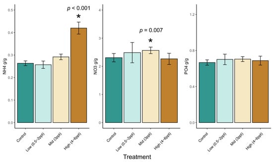
Figure A1.
Soil nutrients (NO3−, NH4+, and PO4−) across binned intermediate salinity treatments. Non-replicated treatments were put into two groups, low (0.5, 1, and 2 ppt) and high (4, 5, and 6 ppt) salinity levels. Controls are green and become more orange with increase in salinity. Ammonium concentrations in soils are significantly greater at salinity ≥3 ppt. Bars are colored by control (dark green), low (light green), 3 ppt (tan), and high (orange) salinity treatments. Asterisks indicate statistically significant differences of salinity treatments to controls Asterisks indicate statistical significance (p ≤ 0.05).
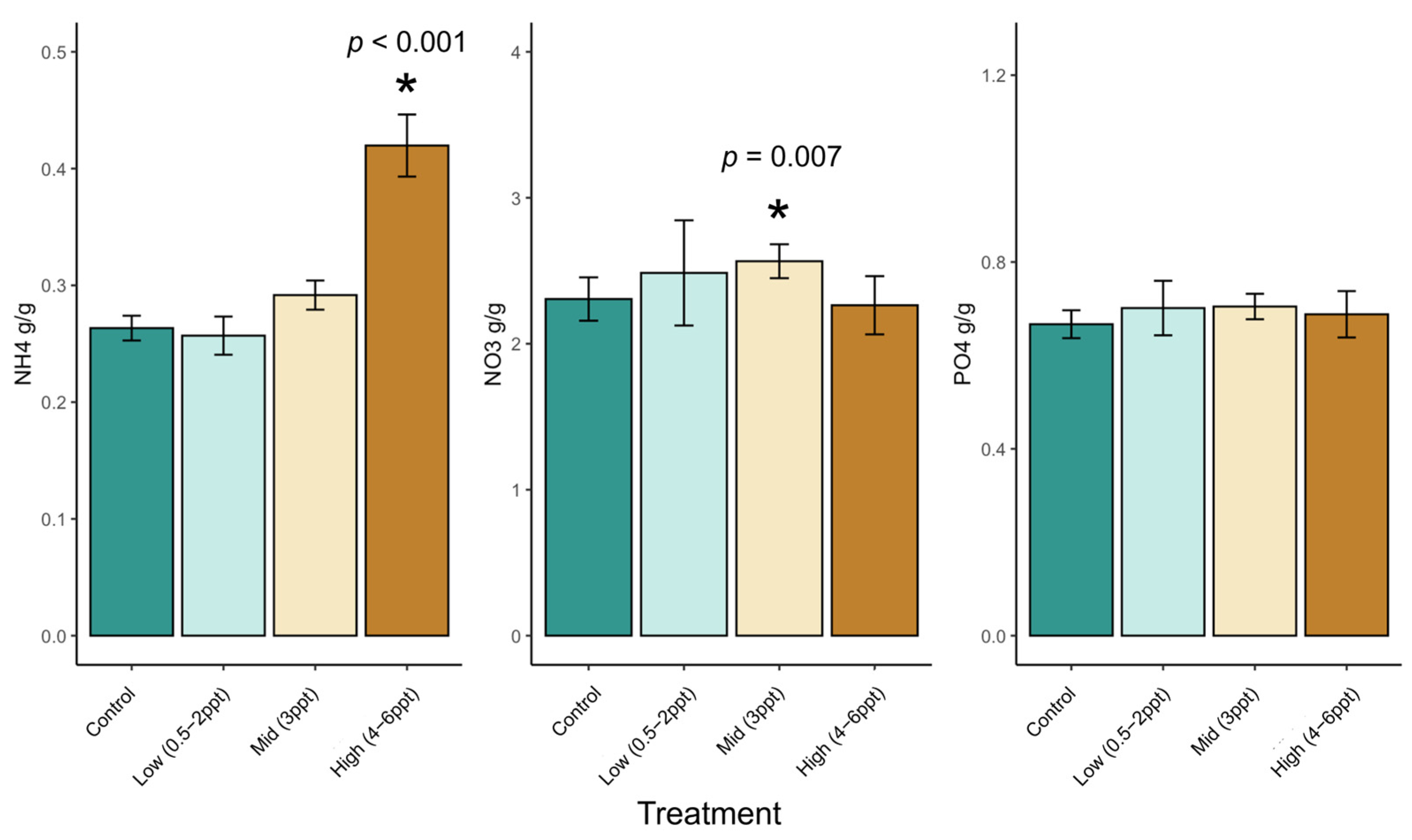
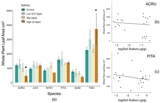
Figure A2.
(a) Total whole-plant leaf area (cm2) by species and binned treatments. Log transformed whole-plant leaf area of (b) Acer rubrum (p = 0.039) and (c) Pinus taeda (p = 0.046) along the soil sodium gradient. Non-replicated treatments were put into two groups, low (0.5, 1, and 2 ppt) and high (4, 5, and 6 ppt) salinity levels. Bars are colored by control (dark green), low (light green), 3 ppt (tan), and high (orange) salinity treatments. Asterisks indicate statistical significance (p ≤ 0.05).

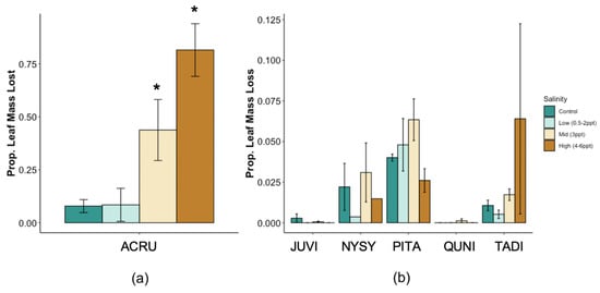
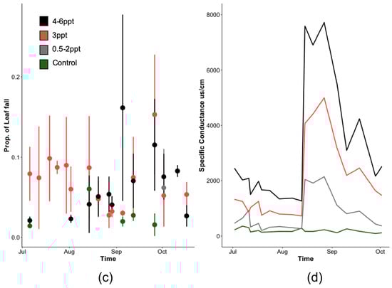
Figure A3.
(a,b) Cumulative leaf loss by species and (c) proportion of Acer rubrum litter fall over the course of this experiment compared to (d) groundwater-specific conductance (µs/cm). Non-replicated treatments were put into two groups, low (0.5, 1, and 2 ppt) and high (4, 5, and 6 ppt) salinity levels (a,b).

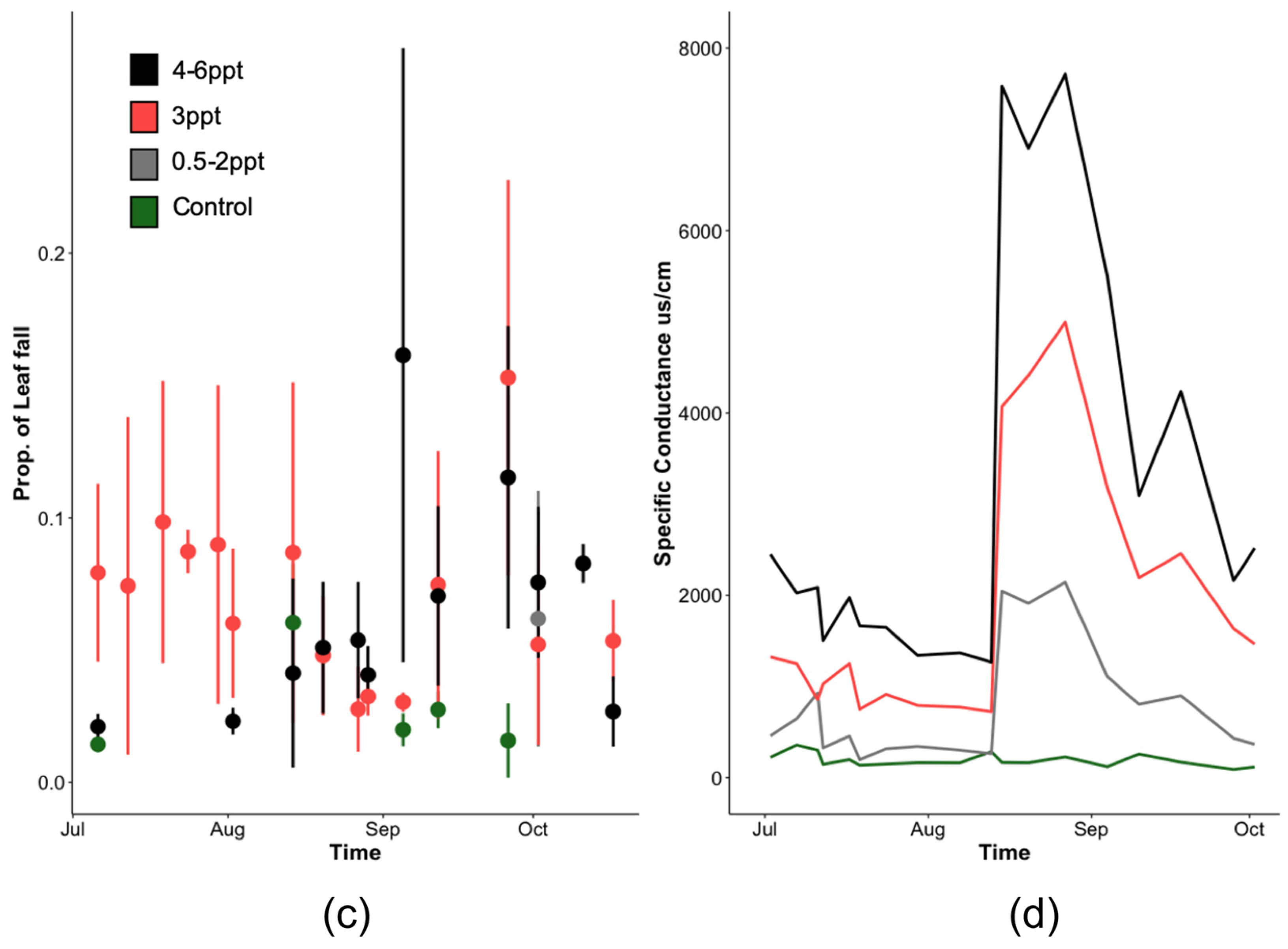
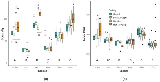
Figure A4.
Comparison of (a) specific leaf area (SLA, leaf area cm3/g dry mass) and (b) leaf dry matter content (LDMC, mg dry leaf mass/g water-saturated fresh leaf mass) within and across all six species and binned salinity treatments (control, low, mid, and high). Non-replicated treatments were put into two groups, low (0.5, 1, and 2 ppt) and high (4, 5, and 6 ppt) salinity levels. Treatments statistically significant (p ≤ 0.05) compared to controls are indicated with an asterisk above the boxplot. Black asterisks below the boxplot indicator significance to other salinity treatment within the bracket. Letters below each set of boxplots per species indicate the statistical significance across species controls. Black points are outliers (values > 1.5 times the interquartile range) included in the statistical analysis.
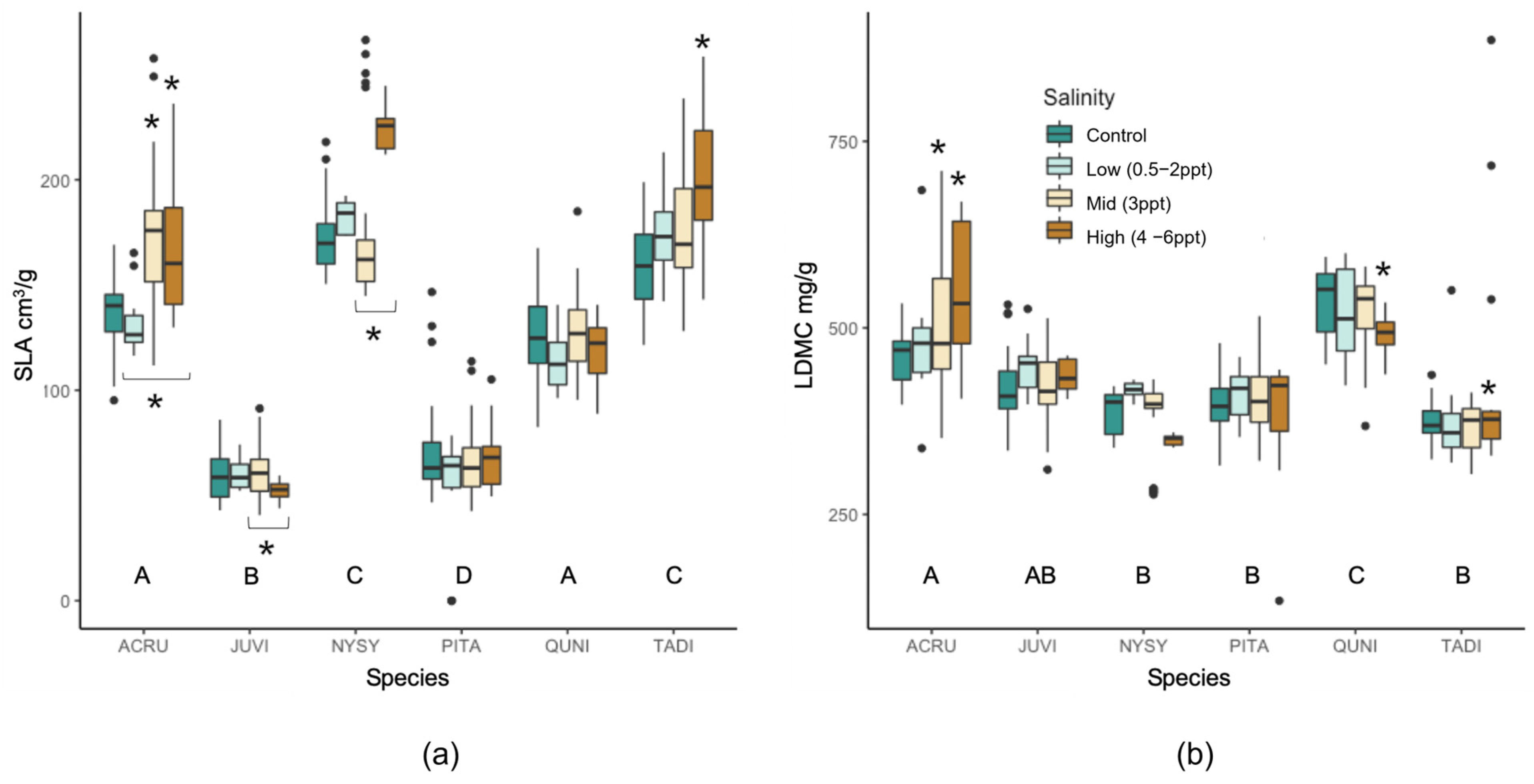

Figure A5.
(a) The relationship between osmotic potential (Ψπ) of the groundwater treatment solutions (NaCl) after the second salinity dose and the difference between Ψπ and predawn leaf water potentials (Ψpd) across the hardwood species and salinity treatments. Each color and shape combination represent Ψπ and Ψpd for each species. The horizontal arrow (color gradient from green to red) represents the direction of salinity increase as Ψπ becomes more negative. The vertical arrow in panel (a) shows that as Ψpd decreases in tandem with a decrease in Ψπ, hydrological flow between the soil and roots reaches equilibrium and ceases to move resulting in leaf loss and mortality. The points closest to zero on the x-axis are controls and salinity treatments increase as they move to the right (more negative Ψπ), noted by the green to red gradient arrow. (b) The relationship between osmotic potential (Ψπ) of the groundwater treatment solutions (NaCl) and the difference between midday water potential (Ψmd) and Ψpd across the hardwood species and salinity treatments. As Ψπ increases (salinity treatments become more saline) hydrological flow between the soil (Ψpd) and light-adapted leaves (Ψmd), equilibrium would be expected (Ψmd − Ψpd = 0; noted by “No H2O Transport”) at high soil salinity, meaning water would ceases to move to more negative pressure potential in the leaves.
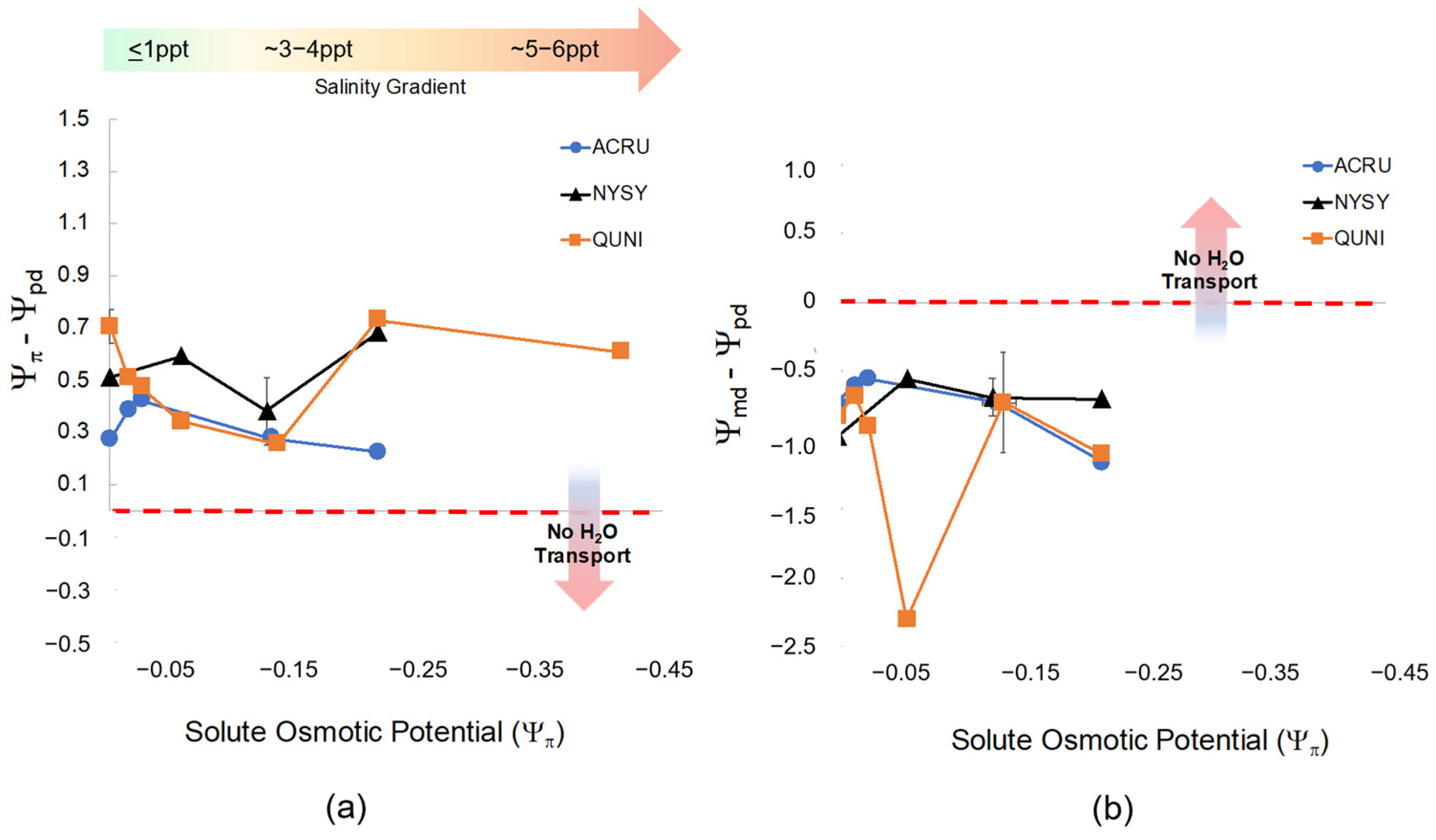
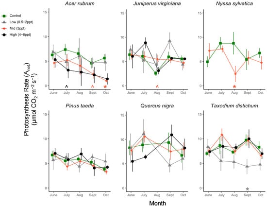
Figure A6.
CO2 assimilation, i.e., photosynthetic rate (Anet, μmol CO2 m−2 s−1), for six tree species from June to October. Significant differences in salinity treatments mean (p ≤ 0.05) from the controls are marked with asterisks, and marginally significant means (p = 0.05–0.1) with hats just above the x-axis at zero, colored by the treatment. Green squares and orange diamonds are the primary replicated salinity treatments (control and 3 ppt, respectively). Non-replicated treatments were put into two groups, low (0.5, 1, and 2 ppt) and high (4, 5, and 6 ppt) salinity levels. Grey triangles and black circles are the low (0.5, 1, and 2 ppt) and high (4, 5, and 6 ppt) treatments. Measurements were taken every month ±5 days from the first day of each month. Points of each measurement are offset for ease of visualization, but all measurements for each species were taken in 1–2 days between 10:00–15:00 h.
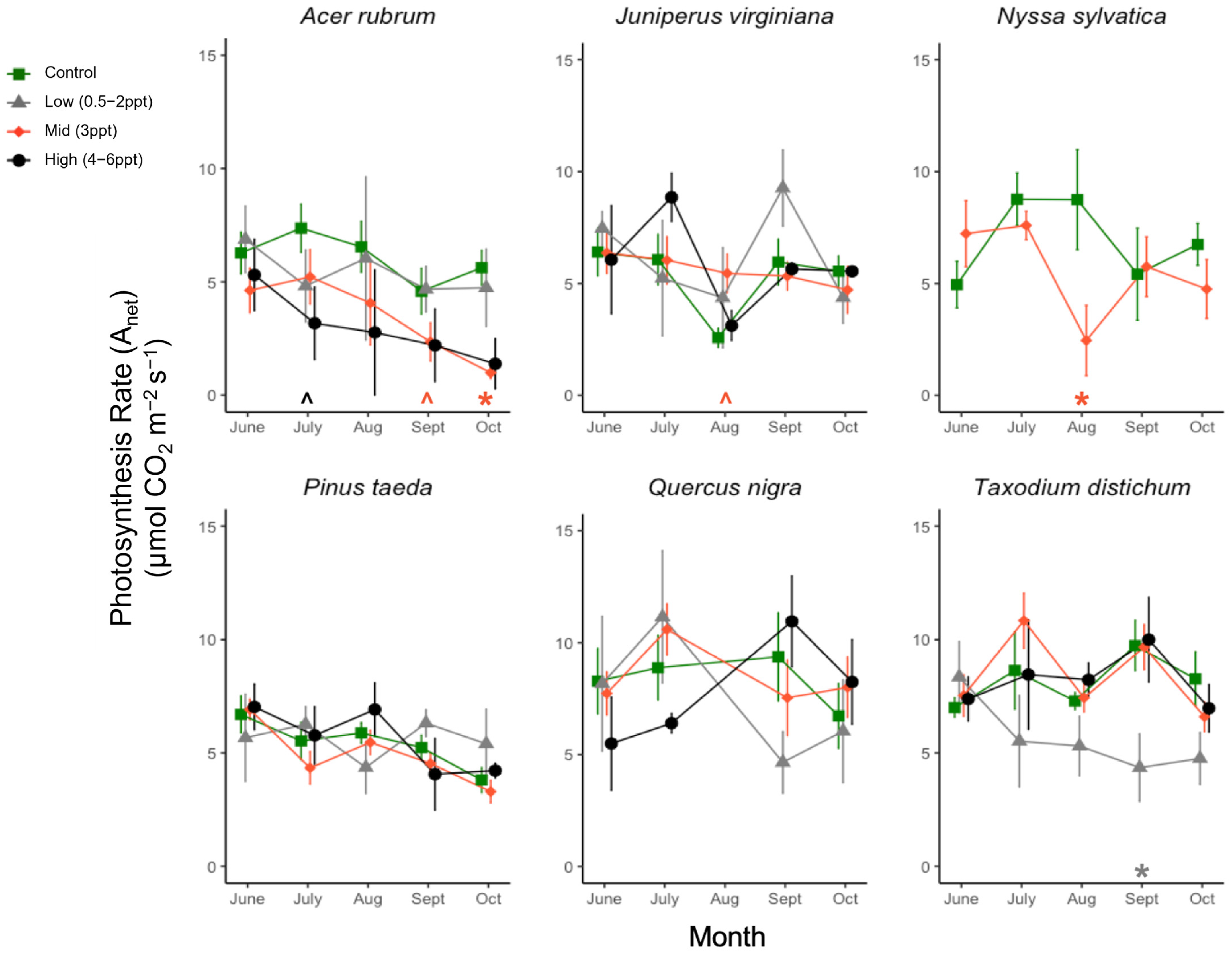
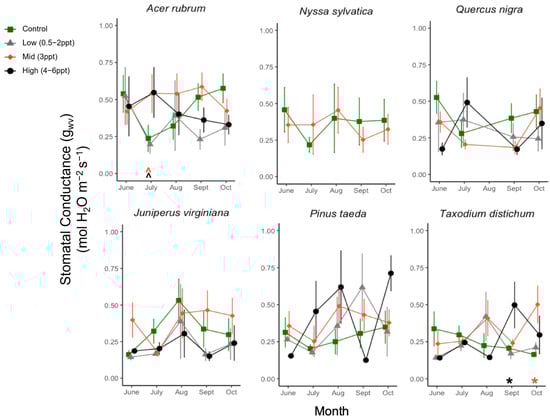
Figure A7.
Stomatal conductance (gs, μmol H2O m−2 s−1) for six tree species from June to October. Significant differences in salinity treatments mean (p ≤ 0.05) from the controls are marked with asterisks, and marginally significant means (p = 0.05–0.1) with hats just above the x-axis at zero, colored by the treatment. Green squares and orange diamonds are the primary replicated salinity treatments (control and 3 ppt, respectively). Non-replicated treatments were put into two groups, low (0.5, 1, and 2 ppt) and high (4, 5, and 6 ppt) salinity levels. Measurements were taken every month ±5 days from the first day of each month. Points of each measurement are offset for ease of visualization, but all measurements for each species were taken in 1–2 days between 10:00–15:00 h.
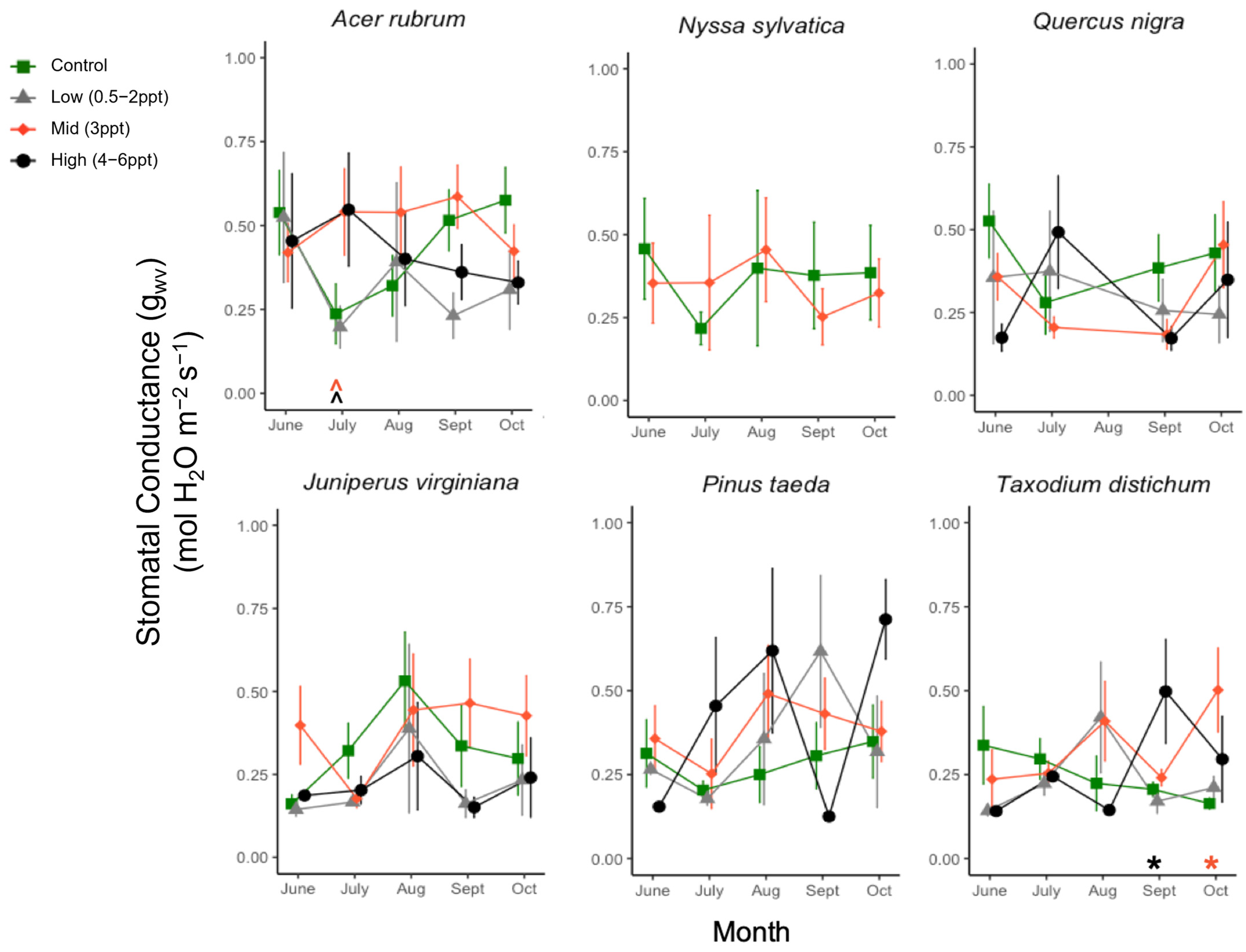
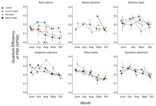
Figure A8.
Quantum efficiency of photosystem II (ΦPSII) of light-adapted leaves all six tree species from June–October 2018 using a pulse-amplitude modulated (PAM) fluorometer chamber for measuring leaf chlorophyll fluorescence and gas exchange simultaneously. Marginal significance in each salinity treatment means (p = 0.05–0.1) from the controls are marked with hats just above the x-axis at zero, colored by the treatment significantly affected by salinity. Green squares and orange diamonds are the primary replicated salinity treatments (control and 3 ppt, respectively). Non-replicated treatments were put into two groups, low (0.5, 1, and 2 ppt) and high (4, 5, and 6 ppt) salinity levels. Measurements were taken every month roughly ±5 days from the first day of each month. Points of each measurement are offset for ease of visualization, but all measurements for each species were taken in 1–2 days between 10:00–15:00 h.
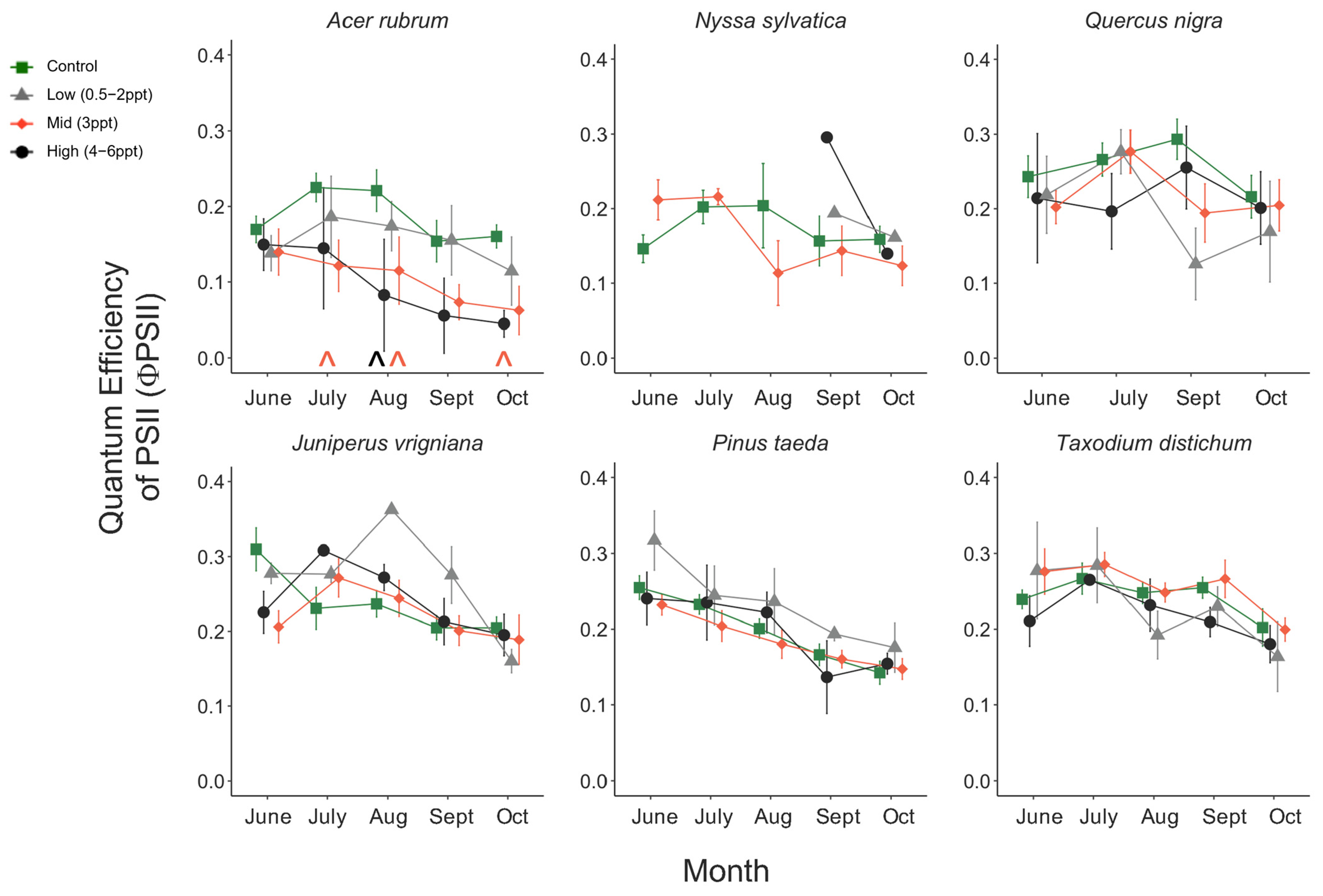
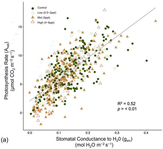
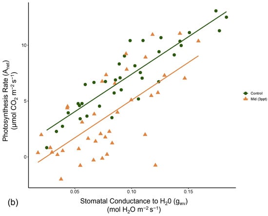
Figure A9.
(a) Linear relationship (R2 = 0.52, p = <0.001) between stomatal conductance (gwv) and photosynthesis rate (Anet) across all 6 species (Acer rubrum, Juniper virginiana, Nyssa sylvatica, Pinus taeda, Quercus nigra, and Taxodium distichum) and binned by salinity treatments (control, low (0.5–2 ppt), mid (3 ppt), and high (4–6 ppt)). Control trees are indicated by green circles, 0.5–2 ppt salinity by light green hollow circles, 3 ppt salinity by orange triangles, and 4–6 ppt by red hollow triangles. (b) Linear relationship (R2 = 0.59, p = <0.01) between stomatal conductance (gwv) and photosynthesis rate (Anet) of Acer rubrum in the two replicated salinity treatments: controls (green circles) and 3 ppt (orange triangles).
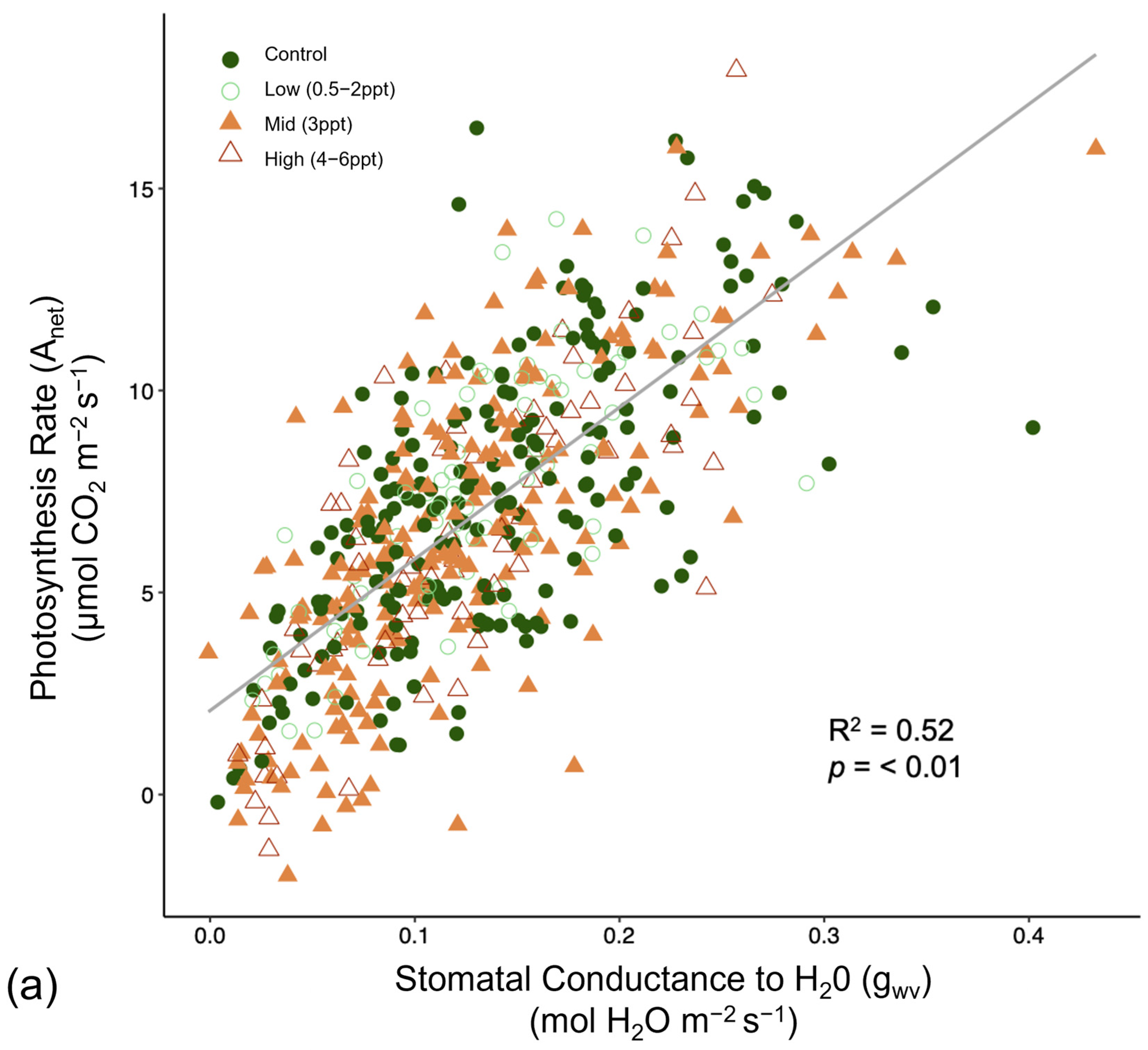
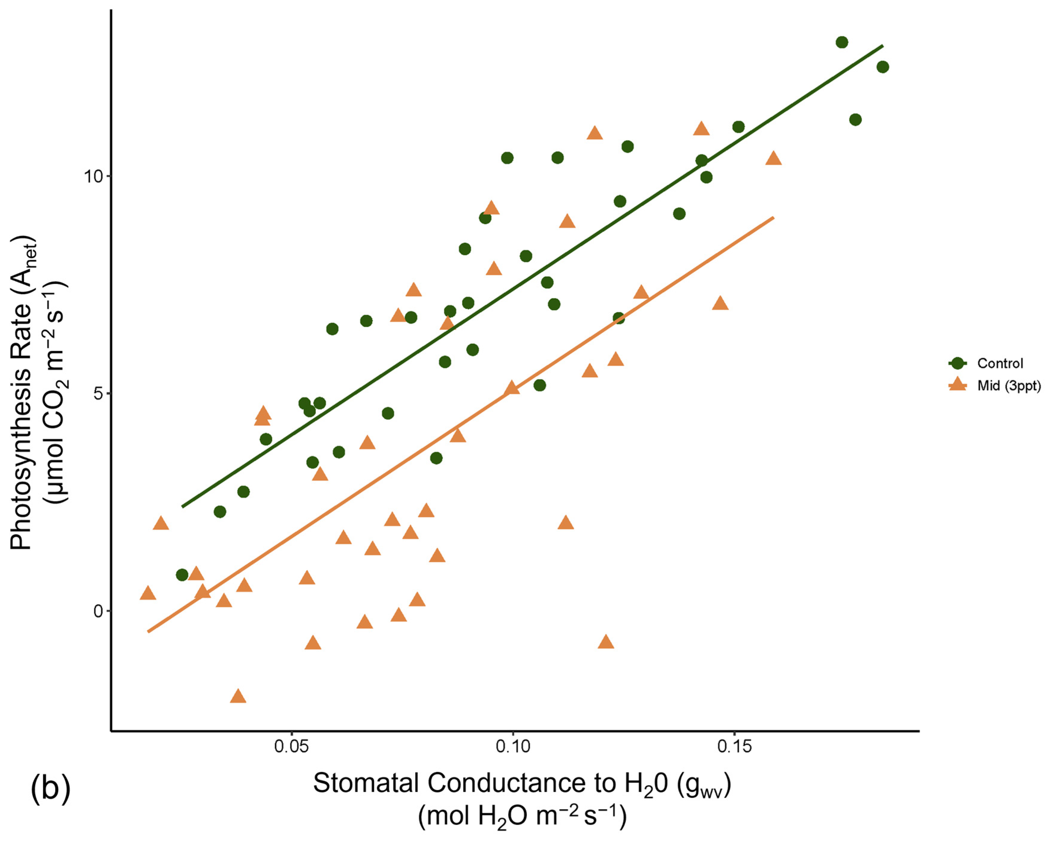
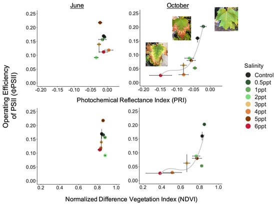
Figure A10.
Operating efficiency of photosystem II (Φ PSII) in light-adapted Acer rubrum leaves as a function of photochemical reflectance index (PRI) (top row) and normalized difference vegetation index (NDVI) (bottom row) in June, September, and October 2018. Each point is the mean of each of the eight salinity treatments, with horizontal and vertical error bars as standard errors (0.95 CI). Non-linear regression lines (dark grey) are significant relationship (October 2018).
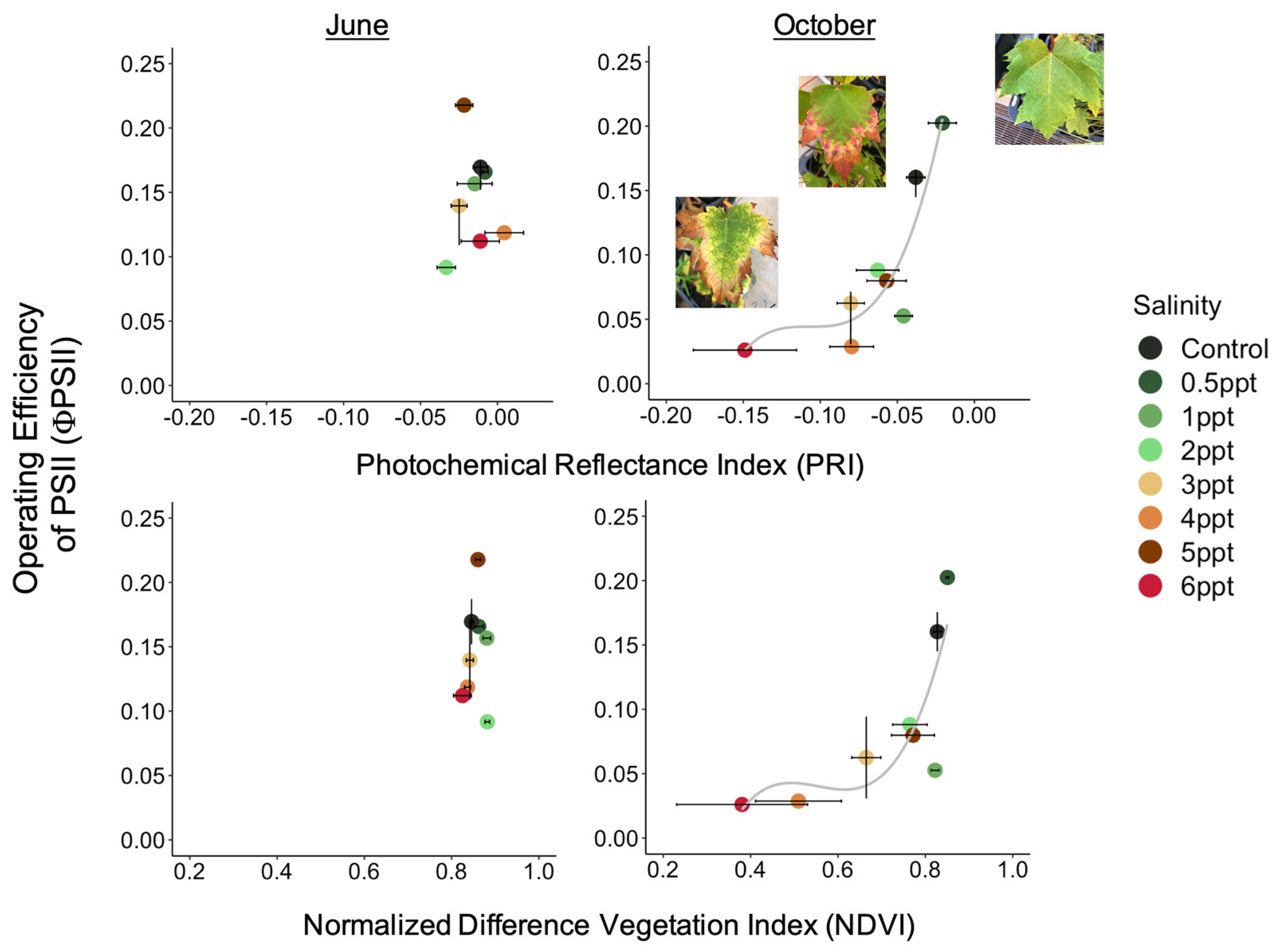
References
- Tully, K.; Gedan, K.; Epanchin-Niell, R.; Strong, A.; Bernhardt, E.S.; Bendor, T.; Mitchell, M.; Kominoski, J.; Jordan, T.E.; Neubauer, S.C.; et al. The Invisible Flood: The Chemistry, Ecology, and Social Implications of Coastal Saltwater Intrusion. BioScience 2019, 69, 368–378. [Google Scholar] [CrossRef]
- Kirwan, M.L.; Gedan, K.B. Sea-Level Driven Land Conversion and the Formation of Ghost Forests. Nat. Clim. Chang. 2019, 9, 450–457. [Google Scholar] [CrossRef]
- Williams, K.; Macdonald, M.; Da Silveira, L.; Sternberg, L. Interactions of Storm, Drought, and Sea-Level Rise on Coastal Forest: A Case Study. J. Coast. Res. 2003, 19, 1116–1121. [Google Scholar]
- White, E.E., Jr.; Ury, E.A.; Bernhardt, E.S.; Yang, X. Climate Change Driving Widespread Loss of Coastal Forested Wetlands Throughout the North American Coastal Plain. Ecosystems 2021, 25, 812–827. [Google Scholar] [CrossRef]
- Munns, R.; Tester, M. Mechanisms of Salinity Tolerance. Annu. Rev. Plant Biol. 2008, 59, 651–681. [Google Scholar] [CrossRef] [PubMed]
- Parida, A.K.; Das, A.B. Salt Tolerance and Salinity Effects on Plants: A Review. Ecotoxicol. Environ. Saf. 2005, 60, 324–349. [Google Scholar] [CrossRef]
- Duberstein, J.A.; Krauss, K.W.; Baldwin, M.J.; Allen, S.T.; Conner, W.H.; Salter, J.S.; Miloshis, M. Small Gradients in Salinity Have Large Effects on Stand Water Use in Freshwater Wetland Forests. For. Ecol. Manag. 2020, 473, 118308. [Google Scholar] [CrossRef]
- Ollinger, S.V. Sources of Variability in Canopy Reflectance and the Convergent Properties of Plants. New Phytol. 2011, 189, 375–394. [Google Scholar] [CrossRef]
- Zhang, T.T.; Zeng, S.L.; Gao, Y.; Ouyang, Z.T.; Li, B.; Fang, C.M.; Zhao, B. Using Hyperspectral Vegetation Indices as a Proxy to Monitor Soil Salinity. Ecol. Indic. 2011, 11, 1552–1562. [Google Scholar] [CrossRef]
- Anderson, S.M.; Ury, E.A.; Taillie, P.J.; Ungberg, E.A.; Moorman, C.E.; Poulter, B.; Ardón, M.; Bernhardt, E.S.; Wright, J.P. Salinity Thresholds for Understory Plants in Coastal Wetlands. Plant Ecol. 2022, 223, 323–337. [Google Scholar] [CrossRef]
- Parihar, P.; Singh, S.; Singh, R.; Singh, V.P.; Prasad, S.M. Effect of Salinity Stress on Plants and Its Tolerance Strategies: A Review. Environ. Sci. Pollut. Res. 2015, 22, 4056–4075. [Google Scholar] [CrossRef]
- Tolliver, K.S.; Martin, D.W.; Young, D.R. Freshwater and Saltwater Flooding Response for Woody Species Common to Barrier Island Swales. Wetlands 1997, 17, 10–18. [Google Scholar] [CrossRef]
- Elmqvist, T.; Folke, C.; Nystrom, M.; Peterson, G.; Bengtsson, J.; Walker, B.; Norberg, J. Response Diversity, Ecosystem Change, and Resilience RID C-1309-2008 RID F-2386-2011. Front. Ecol. Environ. 2003, 1, 488–494. [Google Scholar] [CrossRef]
- van Dijk, G.; Smolders, A.J.P.; Loeb, R.; Bout, A.; Roelofs, J.G.M.; Lamers, L.P.M. Salinization of Coastal Freshwater Wetlands; Effects of Constant versus Fluctuating Salinity on Sediment Biogeochemistry. Biogeochemistry 2015, 126, 71–84. [Google Scholar] [CrossRef]
- Isayenkov, S.V.; Maathuis, F.J.M. Plant Salinity Stress: Many Unanswered Questions Remain. Front. Plant Sci. 2019, 10, 80. [Google Scholar] [CrossRef]
- Brewer, T. Remote Sensing of Vegetation: Principles, Techniques and Applications. Soil Use Manag. 2012, 28, 134. [Google Scholar] [CrossRef]
- Kozlowski, T.T. Responses of Woody Plants to Flooding and Salinity. Tree Physiol. Mon. 1997, 17, 490. [Google Scholar]
- Domec, J.-C.; King, J.S.; Carmichael, M.J.; Overby, A.T.; Wortemann, R.; Smith, W.K.; Miao, G.; Noormets, A.; Johnson, D.M. Aquaporins, and Not Changes in Root Structure, Provide New Insights into Physiological Responses to Drought, Flooding, and Salinity. J. Exp. Bot. 2021, 72, 4489–4501. [Google Scholar] [CrossRef]
- Conner, W.H. The Effect of Salinity and Waterlogging on Growth and Survival of Baldcypress and Chinese Tallow Seedlings. J. Coast. Res. 1994, 10, 1045–1049. [Google Scholar]
- Poulter, B.; Christensen, N.L.; Qian, S.S. Tolerance of Pinus taeda and Pinus serotina to Low Salinity and Flooding: Implications for Equilibrium Vegetation Dynamics. J. Veg. Sci. 2008, 19, 15–22. [Google Scholar] [CrossRef]
- Stimson, H.C.; Breshears, D.D.; Ustin, S.L.; Kefauver, S.C. Spectral Sensing of Foliar Water Conditions in Two Co-Occurring Conifer Species: Pinus edulis and Juniperus monosperma. Remote Sens. Environ. 2005, 96, 108–118. [Google Scholar] [CrossRef]
- Allen, J.A.; Pezeshki, S.R.; Chambers, J.L. Interaction of Flooding and Salinity Stress on Baldcypress (Taxodium distichum). Tree Physiol. 1996, 16, 307–313. [Google Scholar] [CrossRef] [PubMed]
- Day, R.H.; From, A.S.; Johnson, D.J.; Krauss, K.W. Interactive Effects of Salinity and Hydrology on Radial Growth of Bald Cypress (Taxodium distichum (L.) Rich.) in Coastal Louisiana, USA. Forests 2024, 15, 1258. [Google Scholar] [CrossRef]
- Douglas, B.C.; Peltier, W.R. The Puzzle of Global Sea-Level Rise. Cit. Phys. Today 2002, 55, 11. [Google Scholar] [CrossRef]
- Munns, R.; Passioura, J.B.; Colmer, T.D.; Byrt, C.S. Osmotic Adjustment and Energy Limitations to Plant Growth in Saline Soil. New Phytol. 2019, 225, 1091–1096. [Google Scholar] [CrossRef]
- Pezeshki, S.R. Response of Pinus taeda L. to Soil Flooding and Salinity. Ann. Sci. For. 1992, 49, 149–159. [Google Scholar]
- Naumann, J.C.; Young, D.R.; Anderson, J.E. Leaf Chlorophyll Fluorescence, Reflectance, and Physiological Response to Freshwater and Saltwater Flooding in the Evergreen Shrub, Myrica cerifera. Environ. Exp. Bot. 2008, 63, 402–409. [Google Scholar] [CrossRef]
- Flexas, J.; Medrano, H. Drought-inhibition of Photosynthesis in C3 Plants: Stomatal and Non-stomatal Limitations Revisited. Ann. Bot. 2002, 89, 183–189. [Google Scholar] [CrossRef]
- Powell, A.S.; Jackson, L.; Ardón, M. Disentangling the Effects of Drought, Salinity, and Sulfate on Baldcypress Growth in a Coastal Plain Restored Wetland. Restor. Ecol. 2016, 24, 548–557. [Google Scholar] [CrossRef]
- Stiller, V. Soil Salinity and Drought Alter Wood Density and Vulnerability to Xylem Cavitation of Baldcypress (Taxodium distichum (L.) Rich.) Seedlings. Environ. Exp. Bot. 2009, 67, 164–171. [Google Scholar] [CrossRef]
- Seyfried, G.S.; Chow, A.T.; O’Halloran, T.L. Salinization, Inundation and Tree Mortality Interact to Affect Greenhouse Gas Emissions from Stressed Coastal Forests. Soil Biol. Biochem. 2023, 184, 109101. [Google Scholar] [CrossRef]
- Zhai, L.; Krauss, K.W.; Liu, X.; Duberstein, J.A.; Conner, W.H.; DeAngelis, D.L.; Sternberg, L.d.S.L. Growth Stress Response to Sea Level Rise in Species with Contrasting Functional Traits: A Case Study in Tidal Freshwater Forested Wetlands. Environ. Exp. Bot. 2018, 155, 378–386. [Google Scholar] [CrossRef]
- Brinson, M.M.; Christian, R.R.; Blum, L.K.; Estuaries, S.; Odum, W.E.; Symposium, M.; Blum, L.K. Multiple States in the Sea-Level Induced Transition from Terrestrial Forest to Estuary. Estuaries 1995, 18, 648–659. [Google Scholar]
- Ury, E.A.; Anderson, S.M.; Peet, R.K.; Bernhardt, E.S.; Wright, J.P. Succession, Regression and Loss: Does Evidence of Saltwater Exposure Explain Recent Changes in the Tree Communities of North Carolina’s Coastal Plain? Ann. Bot. 2019, 125, 255–263. [Google Scholar] [CrossRef]
- Carmichael, M.J.; Smith, W.K. Growing Season Ecophysiology of Taxodium distichum (L.) Rich. (Bald cypress) Saplings in a Restored Wetland: A Baseline for Restoration Practice. Botany 2016, 94, 1115–1125. [Google Scholar] [CrossRef]
- Maxwell, K.; Johnson, G.N. Chlorophyll Fluorescence—A Practical Guide. J. Exp. Bot. 2000, 51, 659–668. [Google Scholar] [CrossRef]
- Baker, N.R. Chlorophyll Fluorescence: A Probe of Photosynthesis In Vivo. Annu. Rev. Plant Biol. 2008, 59, 89–113. [Google Scholar] [CrossRef]
- Murchie, E.H.; Lawson, T. Chlorophyll Fluorescence Analysis: A Guide to Good Practice and Understanding Some New Applications. J. Exp. Bot. 2013, 64, 3983–3998. [Google Scholar] [CrossRef]
- Zinnert, J.C.; Nelson, J.D.; Hoffman, A.M. Effects of Salinity on Physiological Responses and the Photochemical Reflectance Index in Two Co-Occurring Coastal Shrubs. Plant Soil 2012, 354, 45–55. [Google Scholar] [CrossRef]
- Naumann, J.C.; Anderson, J.E.; Young, D.R. Linking Physiological Responses, Chlorophyll Fluorescence and Hyperspectral Imagery to Detect Salinity Stress Using the Physiological Reflectance Index in the Coastal Shrub, Myrica cerifera. Remote Sens. Environ. 2008, 112, 3865–3875. [Google Scholar] [CrossRef]
- Negrão, S.; Schmöckel, S.M.; Tester, M. Evaluating Physiological Responses of Plants to Salinity Stress. Ann. Bot. 2017, 119, 1–11. [Google Scholar] [CrossRef] [PubMed]
- Peñuelas, J.; Filella, L. Technical Focus: Visible and near-Infrared Reflectance Techniques for Diagnosing Plant Physiological Status. Trends Plant Sci. 1998, 3, 151–156. [Google Scholar] [CrossRef]
- Naumann, J.C.; Young, D.R.; Anderson, J.E. Spatial Variations in Salinity Stress across a Coastal Landscape Using Vegetation Indices Derived from Hyperspectral Imagery. Plant Ecol. 2009, 202, 285–297. [Google Scholar] [CrossRef]
- Pezeshki, S.R.; Delaune, R.D.; Patrick, W.H. Flooding and Saltwater Intrusion: Potential Effects on Survival and Productivity of Wetland Forests along the U.S. Gulf Coast. For. Ecol. Manag. 1990, 33–34, 287–301. [Google Scholar] [CrossRef]
- Krauss, K.W.; Duberstein, J.A.; Doyle, T.W.; Conner, W.H.; Day, R.H.; Inabinette, L.W.; Whitbeck, J.L. Site Condition, Structure, and Growth of Baldcypress along Tidal/Non-Tidal Salinity Gradients. Wetlands 2009, 29, 505–519. [Google Scholar] [CrossRef]
- McLeod, K.W.; McCarron, J.K.; Conner, W.H. Photosynthesis and Water Relations of Four Oak Species: Impact of Flooding and Salinity. Trees 1999, 13, 178. [Google Scholar] [CrossRef]
- Waters, P.; Dahl, E. Nordic Society Oikos Ecological Salinity Boundaries. Nord. Soc. Oikos 1956, 7, 1–21. [Google Scholar]
- Ardón, M.; Morse, J.L.; Colman, B.P.; Bernhardt, E.S. Drought-Induced Saltwater Incursion Leads to Increased Wetland Nitrogen Export. Glob. Chang. Biol. 2013, 19, 2976–2985. [Google Scholar] [CrossRef]
- Pérez-Harguindeguy, N.; Díaz, S.; Garnier, E.; Lavorel, S.; Poorter, H.; Jaureguiberry, P.; Bret-Harte, M.S.; Cornwell, W.K.; Craine, J.M.; Gurvich, D.E.; et al. Corrigendum: New Handbook for Standardised Measurement of Plant Functional Traits Worldwide (Australian Journal of Botany (2013) 61:3 (167–234) DOI: 10.1071/BT12225). Aust. J. Bot. 2016, 64, 715–716. [Google Scholar] [CrossRef]
- Naumann, J.C.; Young, D.R.; Anderson, J.E. Linking Leaf Chlorophyll Fluorescence Properties to Physiological Responses for Detection of Salt and Drought Stress in Coastal Plant Species. Physiol. Plant. 2007, 131, 422–433. [Google Scholar] [CrossRef]
- Richter, H. Water Relations of Plants in the Field: Some Comments on the Measurement of Selected Parameters. J. Exp. Bot. 1997, 48, 1–7. [Google Scholar] [CrossRef]
- Heberling, J.M.; Fridley, J.D. Invaders Do Not Require High Resource Levels to Maintain Physiological Advantages in a Temperate Deciduous Forest. Ecology 2016, 97, 874–884. [Google Scholar] [CrossRef] [PubMed]
- Farquhar, G.D.; O’Leary, M.H.; Berry, J.A. On the Relationship between Carbon Isotope Discrimination and the Intercellular Carbon Dioxide Concentration in Leaves. Aust. J. Plant Physiol. 1982, 9, 121–137. [Google Scholar] [CrossRef]
- R Core Team. R: A Language and Environment for Statistical Computing; R Foundation for Statistical Computing: Vienna, Austria, 2019. [Google Scholar]
- Penuelas, J.; Llusia, J.; Pinol, J.; Filella, I. Photochemical Reflectance Index and Leaf Photosynthetic Radiation-Use-Efficiency Assessment in Mediterranean Trees. Int. J. Remote Sens. 1997, 18, 2863–2868. [Google Scholar] [CrossRef]
- Gamon, J.A.; Peñuelas, J.; Field, C.B. A Narrow-Waveband Spectral Index That Tracks Diurnal Changes in Photosynthetic Efficiency. Remote Sens. Environ. 1992, 41, 35–44. [Google Scholar] [CrossRef]
- Koc, A.; Henriksson, T.; Chawade, A. Specalyzer-An Interactive Online Tool to Analyze Spectral Reflectance Measurements. PeerJ 2018, 2018, e5031. [Google Scholar] [CrossRef]
- Bates, D.; Mächler, M.; Bolker, B.; Walker, S. Fitting Linear Mixed-Effects Models Using Lme4. J. Stat. Softw. 2015, 67, 1–48. [Google Scholar] [CrossRef]
- Wickham, H.; Chang, W.; Henry, L.; Pedersen, T.L.; Takahashi, K.; Wilke, C.; Woo, K.; Yutani, H.; Dunnington, D.; van den Brand, T.; et al. Ggplot2: Create Elegant Data Visualisations Using the Grammar of Graphics 2024. Available online: https://ggplot2.tidyverse.org/reference/ggplot2-package.html (accessed on 19 October 2018).
- RStudio Team. RStudio: Integrated Development for R; RStudio, Inc.: Boston, MA, USA, 2019; Available online: http://www.rstudio.com/ (accessed on 19 October 2018).
- Krings, A. Contributions to the Flora of Nags Head Woods, I: Key to the Trees and Shrubs. Vulpia 2003, 2, 1–14. [Google Scholar]
- Conner, W.H.; Askew, G.R. Impact of Saltwater Flooding on Red Maple, Redbay, and Chinese Tallo Seedlings. Castanea 1993, 58, 214–219. [Google Scholar]
- Poulter, B.; Qian, S.S.; Christensen, N.L. Determinants of Coastal Treeline and the Role of Abiotic and Biotic Interactions. Plant Ecol. 2009, 202, 55–66. [Google Scholar] [CrossRef]
- Ahmad, P.; Prasad, M.N.V.; Azooz, M.M. Salt Stress in Plants: Signalling, Omics and Adaptations; Springer: Berlin/Heidelberg, Germany, 2014; ISBN 978-1-4614-6108-1. [Google Scholar]
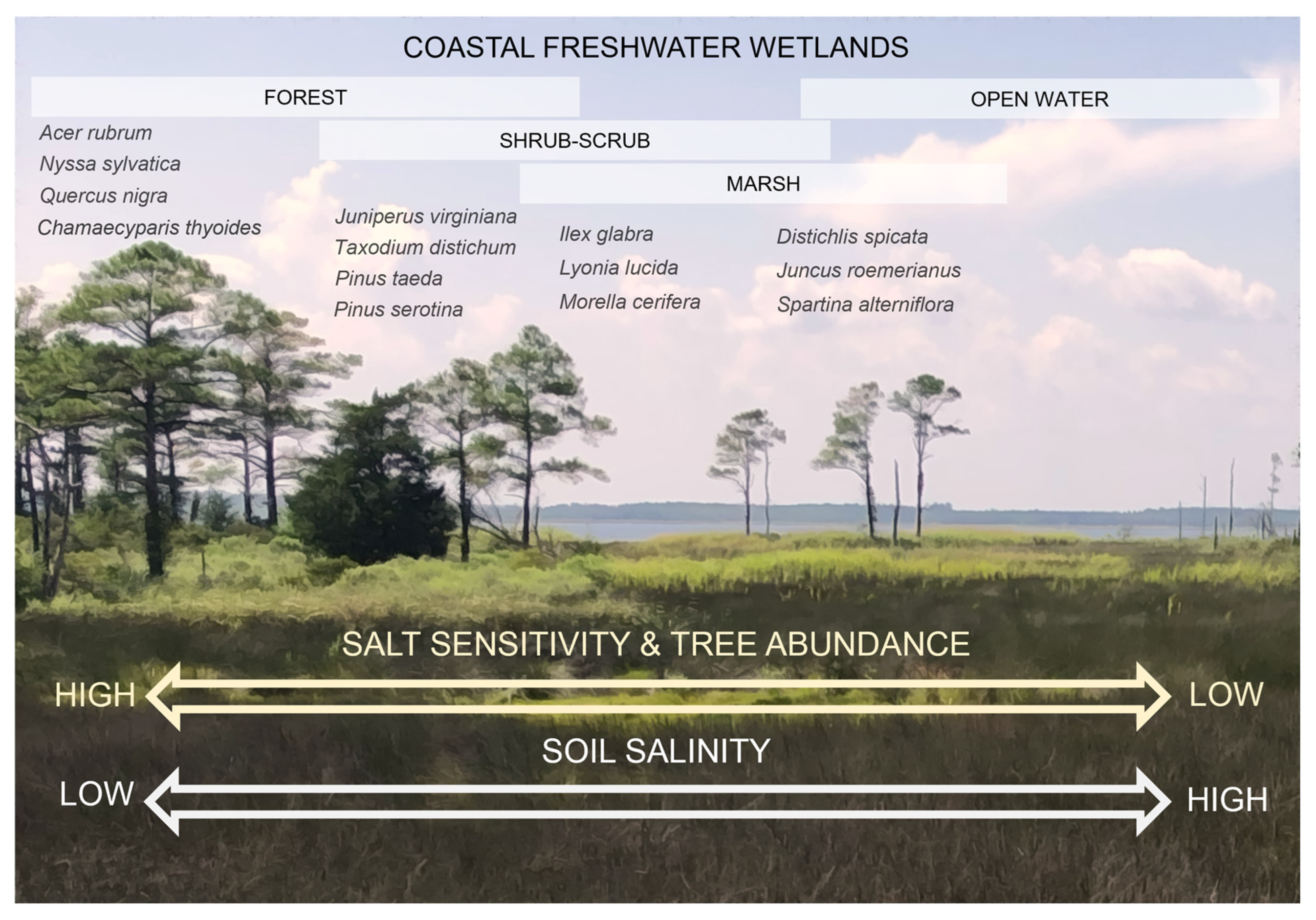
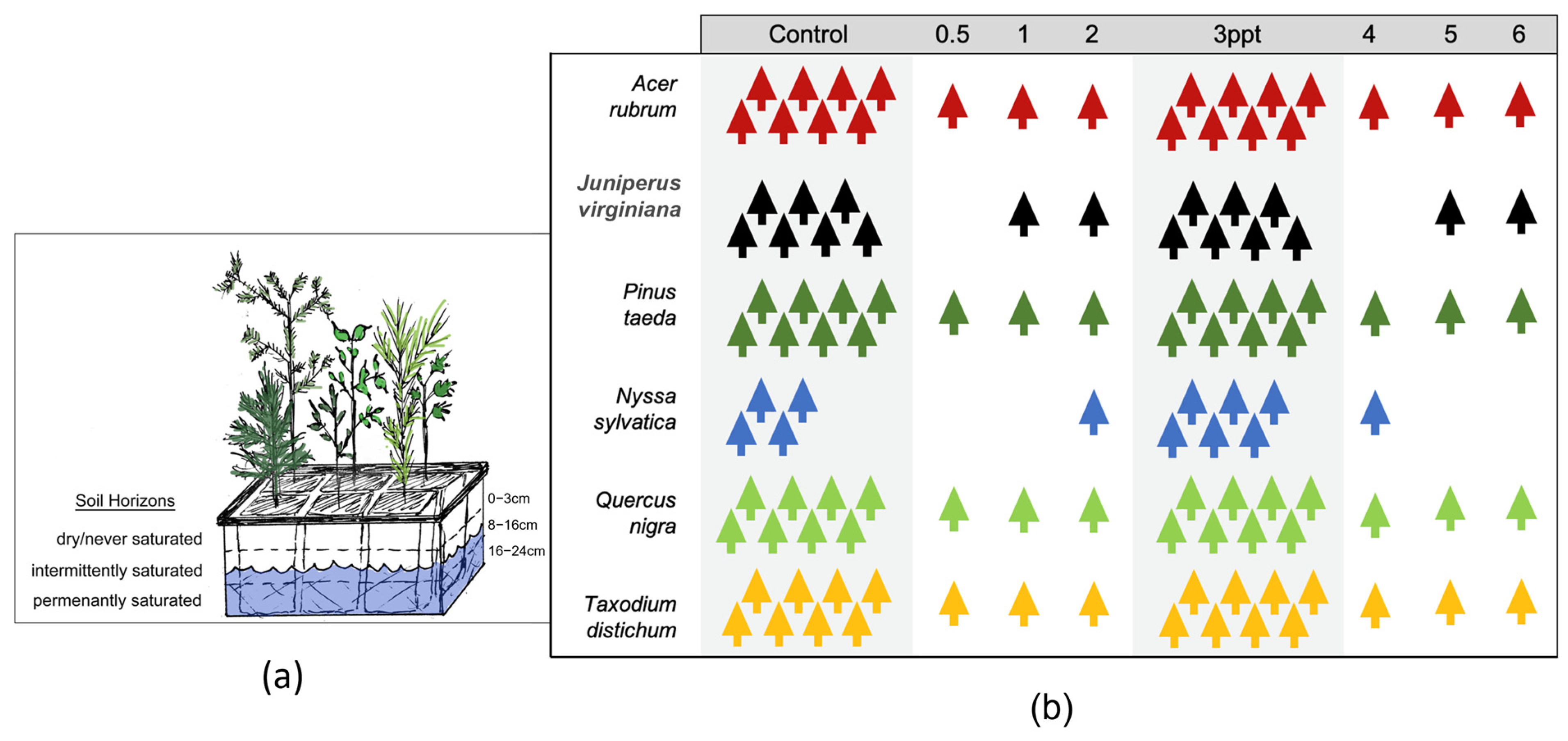
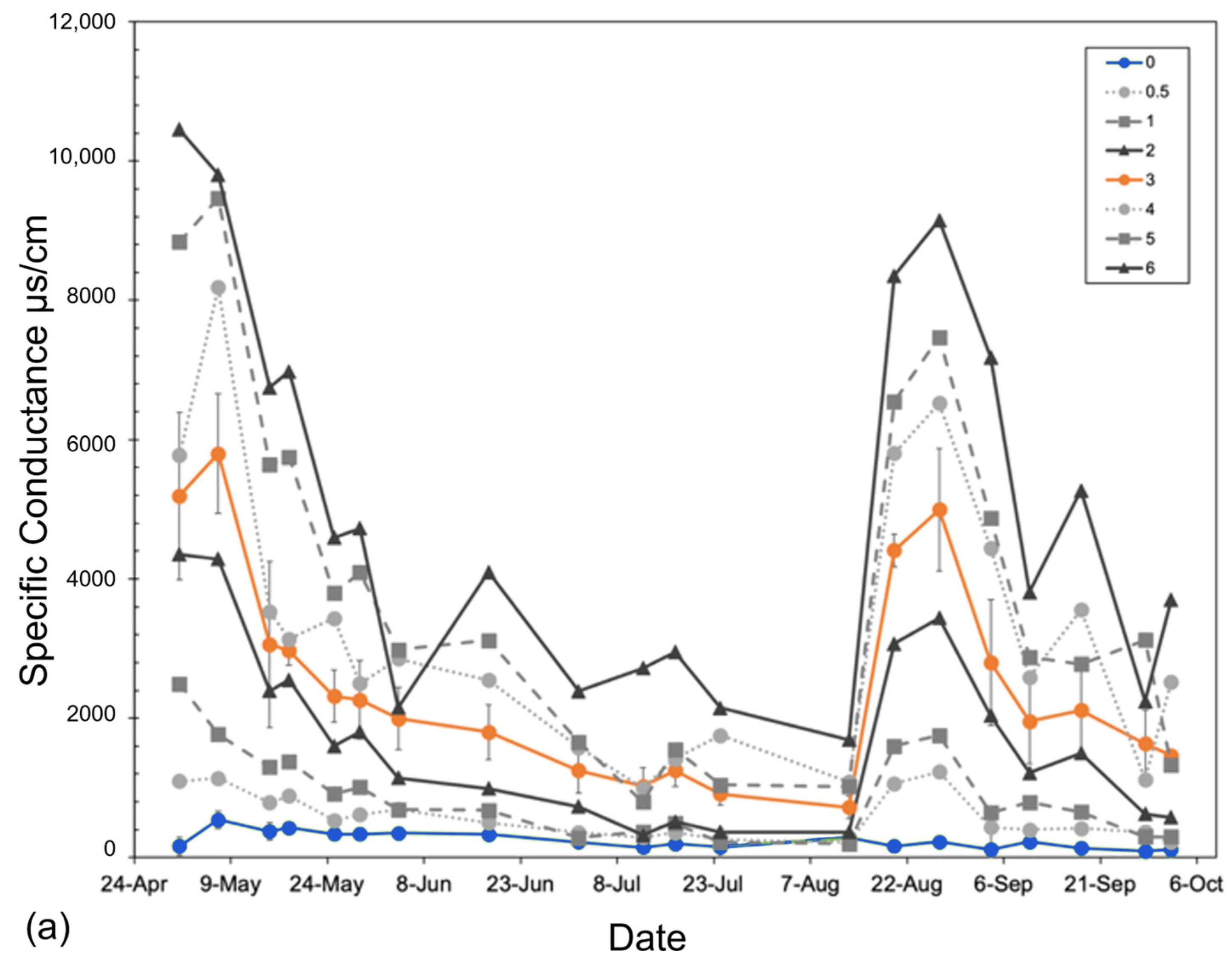
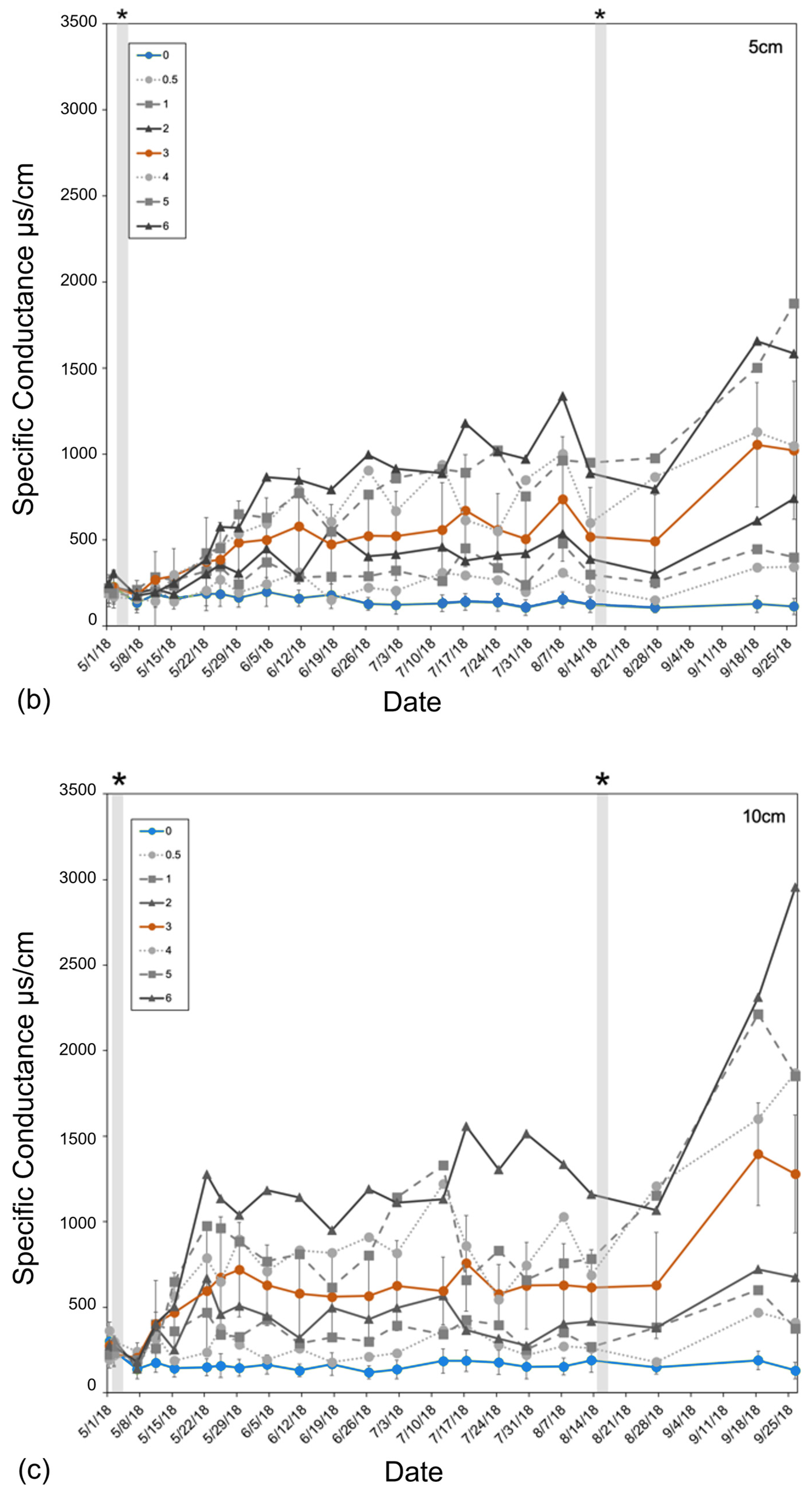
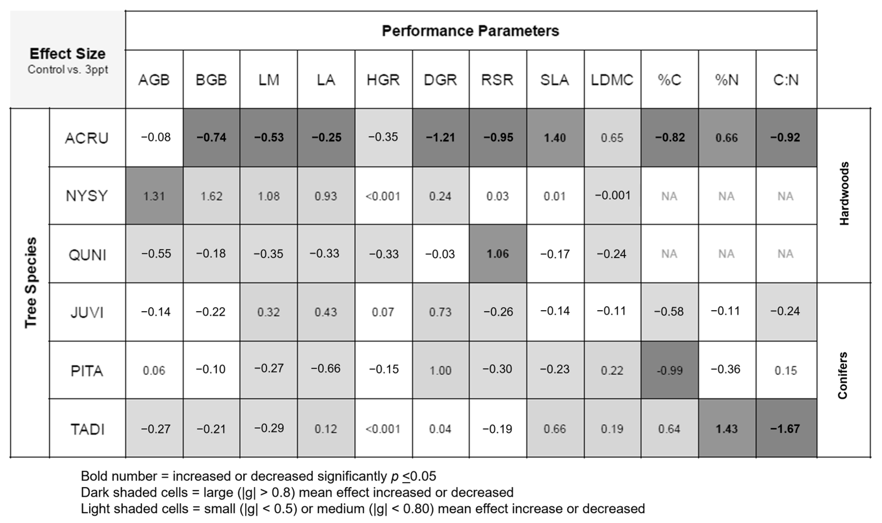
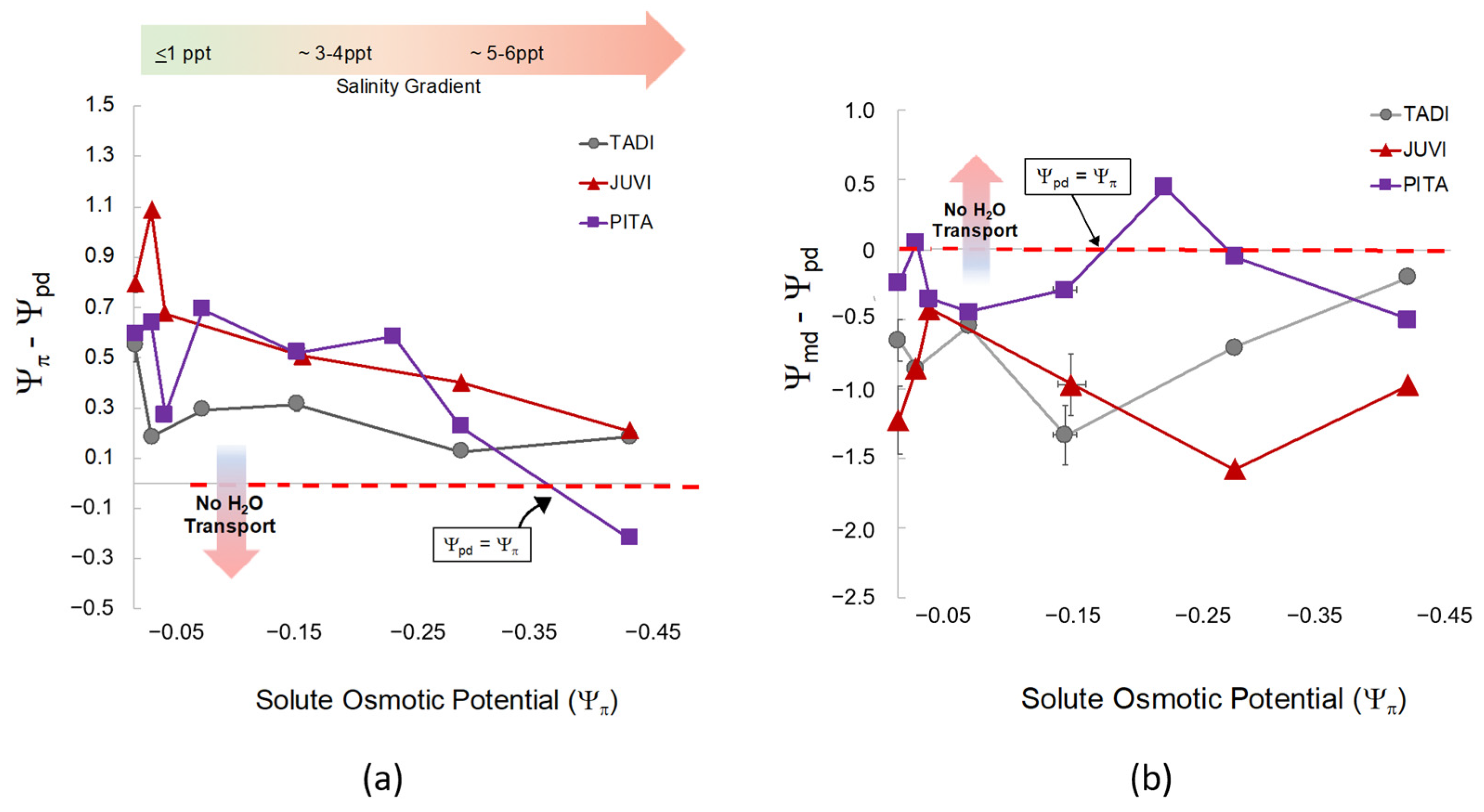
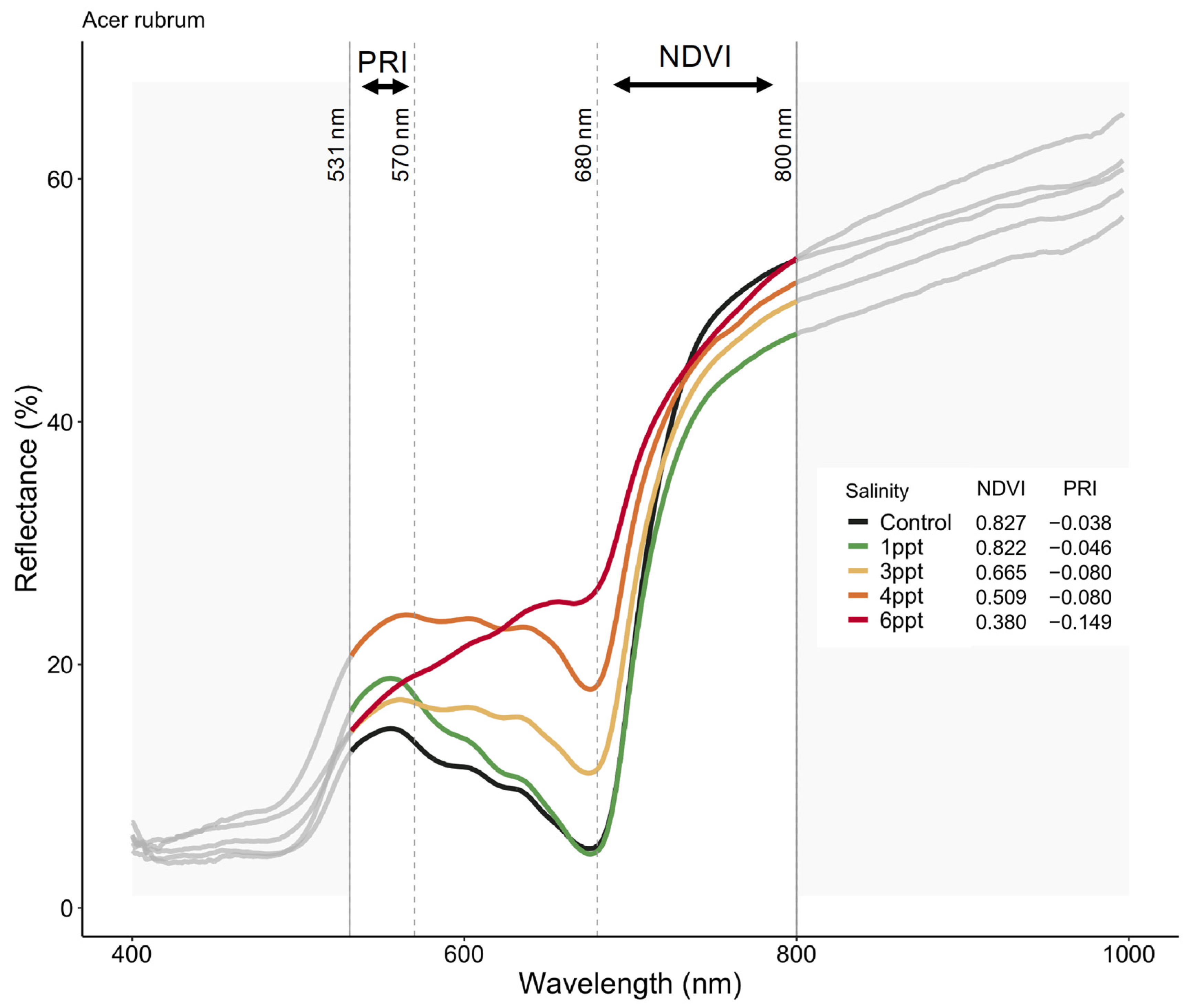
Disclaimer/Publisher’s Note: The statements, opinions and data contained in all publications are solely those of the individual author(s) and contributor(s) and not of MDPI and/or the editor(s). MDPI and/or the editor(s) disclaim responsibility for any injury to people or property resulting from any ideas, methods, instructions or products referred to in the content. |
© 2024 by the authors. Licensee MDPI, Basel, Switzerland. This article is an open access article distributed under the terms and conditions of the Creative Commons Attribution (CC BY) license (https://creativecommons.org/licenses/by/4.0/).