Abstract
Airborne Laser Scanning (ALS) metrics have been used to develop area-based forest inventories; these metrics generally include estimates of stand-level, per hectare values and mean tree attributes. Tree-based ALS inventories contain desirable information on individual tree dimensions and how much they vary within a stand. Adding size class distribution information to area-based inventories helps to bridge the gap between area- and tree-based inventories. This study examines the potential of ALS and stereo-imagery point clouds to predict size class distributions in a boreal forest. With an accurate digital terrain model, both ALS and imagery point clouds can be used to estimate size class distributions with comparable accuracy. Nonparametric imputations were generally superior to parametric imputations; this may be related to the limitation of using a unimodal Weibull function on a relatively small prediction unit (e.g., 400 m2).
1. Introduction
Forest Resource Inventories in Ontario have been designed to meet long-term (20 year) strategic management planning needs and have traditionally contained photo-interpreted estimates of species composition, age, height, and site occupancy. Recent studies have shown that these data may be augmented with area-based estimates of growing stock (basal area, volume) and average tree size (height, diameter, volume) derived from either Airborne Laser Scanning (ALS) [1,2] or stereo image point clouds (IPC) [3], to facilitate tactical (5-year) and operational (1-year) planning of forest operations. Since harvesting operations have become more mechanized and processing facilities are increasingly optimized for particular products and sizes of raw materials, there is considerable interest in adding information to inventories on the size assortment of the stems.
Modelling, or fitting size class distributions to empirical data, has received considerable attention. Much of the earlier work focused on selection and fitting of an appropriate distribution. Bailey and Dell [4] proposed using the Weibull function for size class distributions. Most of the commonly used distribution functions are unimodal, while many forest size class distributions are irregular and not well characterized by a unimodal function. Mixture models combine two or more distribution functions, resulting in multi-modal distribution functions, which have been used to characterize more complex forests e.g., [5]. Predicting the modeled size class distribution from ancillary data e.g., [6] is generally the next step. This may include ensuring the size class distribution is compatible with other inventory attributes, including total stems and basal area [7]. Alternatively, the Diameter at breast height (Dbh) and height distributions can be predicted together [8]. The advantage of using a parametric distribution model is the typically low (one to four) number of parameters that have to be predicted; the key disadvantage is a restriction in model form [9].
Nearest neighbour imputation methods have become popular in forest inventory efforts [10]. Imputation is used to associate expensive but sparse data with inexpensive and spatially comprehensive data [11]. The response variable is measured on a subset of the prediction units in the population (the reference data set), and auxiliary or predictor variables are available for the entire population. Generally, a prediction for a target unit is calculated from a weighted combination of the response variables from observations in the reference data set that are most similar, or nearest neighbours, to the target in terms of auxiliary variables. Nearest neighbour techniques can be used to predict categorical and continuous variables and univariate or multivariate response variables [10]. This ability to predict multivariate response variables makes nearest neighbour imputation particularly promising for the prediction of probability density functions, particularly for complex stands with multiple species and a variety of tree sizes [12]. The size class distributions for these stands tend to be multimodal and not easily represented by parametric functions [10]. When the reference dataset is large, k-Nearest Neighbour (kNN), estimation shows promise in predicting relatively broad Dbh classes [13]. However, in many forest inventory applications, ground observations are relatively few and are generally captured from small plot areas (typically 400 m2). RandomForest, another nonparametric imputation method, has shown promise in forest application using ALS [14].
ALS has been used to predict size class distributions. When height is the size attribute, early work [15] focused on predicting the distribution of tree heights from the distribution of ALS return heights by first generating a canopy model for the calibration data. The canopy area model or three-dimensional canopy volume model was developed for the calibration data using stem-mapped data, including crown measurements. This canopy model was used to generate a theoretical distribution of ALS returns, which was then compared to the actual returns. More recent work [16,17] also predicted the distribution of canopy heights. Rather than requiring tree location in the calibration data, assumptions were made about the spatial arrangement of the trees. Another approach, particularly when diameter is the size attribute, is to predict the size class distribution directly from ALS data without first generating a crown map. Bollandsås et al. [18] used an ALS point density of ~0.7/m2 in a Norwegian boreal forest to predict the deciles of the Dbh distribution using most similar neighbour (MSN) and seemingly unrelated regression (SUR). The MSN and SUR predictions generated an unbiased prediction of total basal area, but MSN was better at predicting the number of large trees. Some authors have also included predictors from aerial photographs. Packalén and Maltamo [19] used ALS predictors as well as spectral values and textural features from aerial photos that had been radiometrically corrected against a Landsat 7 ETM.
Recently, ALS-like point clouds have been derived from stereo imagery using pixel matching. A previous study compared ALS and IPC for predicting forest inventory attributes in the Ontario boreal forest [3]. Comparable accuracies were obtained for predictions of forest inventory attributes including basal area, merchantable stem volume, top height and quadratic mean Dbh, but they found some loss of precision with the IPC using an area-based modeling approach. To date, no studies have compared the use of ALS and IPC in the prediction of size class distributions.
The objective of this study was to investigate and compare the potential of ALS and IPC metrics to predict size class distributions for a management area in a northeastern Ontario boreal forest. Both parametric and nonparametric approaches are evaluated in this comparison.
2. Materials
The study area and data were used in a previous study [3] to estimate traditional forest inventory attributes.
2.1. Study Area
The Hearst Forest is located in northeastern Ontario (Figure 1) and has more than 1,000,000 ha of productive forest, classified into eight forest types (Table 1). The following description is detailed in the 2007 forest management plan [20]. The predominant tree species on the Hearst Forest is black spruce (Picea mariana Mill. B.S.P.). Sixty-seven percent of the land base is composed of forest types in which black spruce is a major component. The better-drained, more productive lowland transitional and upland sites, where the Spruce Pine (SP) and Spruce Fir (SF) forest types are found, make up 30 percent of the land base. On these sites, black spruce may be found with white spruce (Picea glauca (Moench) A. Voss), jack pine (Pinus banksiana Lamb.), balsam fir (Abies balsamea (L.) Mill), and trembling aspen (Populus tremulodies Michx.). The black spruce (SB) forest type makes up 34 percent of the land base and consists of black spruce on lowland areas in pure stands and in association with cedar (Thuja occidentalis L.) and tamarack (Larix laricina (Du Roi) K. Koch). These lowland sites are characterized by poor drainage and moderately-deep to deep (more than 20 cm) organic soil over clay. The productivity of these areas is low to moderate. Lowland conifer (LC) makes up about 3 percent of the area and is a very wet but well drained forest type with strong groundwater seepage dominated by black spruce and often supporting cedar, tamarack and white spruce. Approximately 25 percent of the land base occurs on mineral soils on upland sites associated with mixedwood stands consisting of jack pine, black and white spruce, trembling aspen, balsam poplar (Populus balsamifera L.), white birch (Betula papyrifera Marsh.) and balsam fir. The soils are fine loam to sandy clay, topped by less than 20 cm of organic material. The mixedwood forest type is split into mixedwood conifer (MWC) or mixedwood hardwood (MWH), depending on whether conifers or hardwoods are the majority. Intolerant hardwoods (IH) make up 5.5 percent of the land base and consist mainly of trembling aspen and white birch. Approximately 3 percent of the land base consists of stands that are dominated by jack pine on mineral soils (PJ).
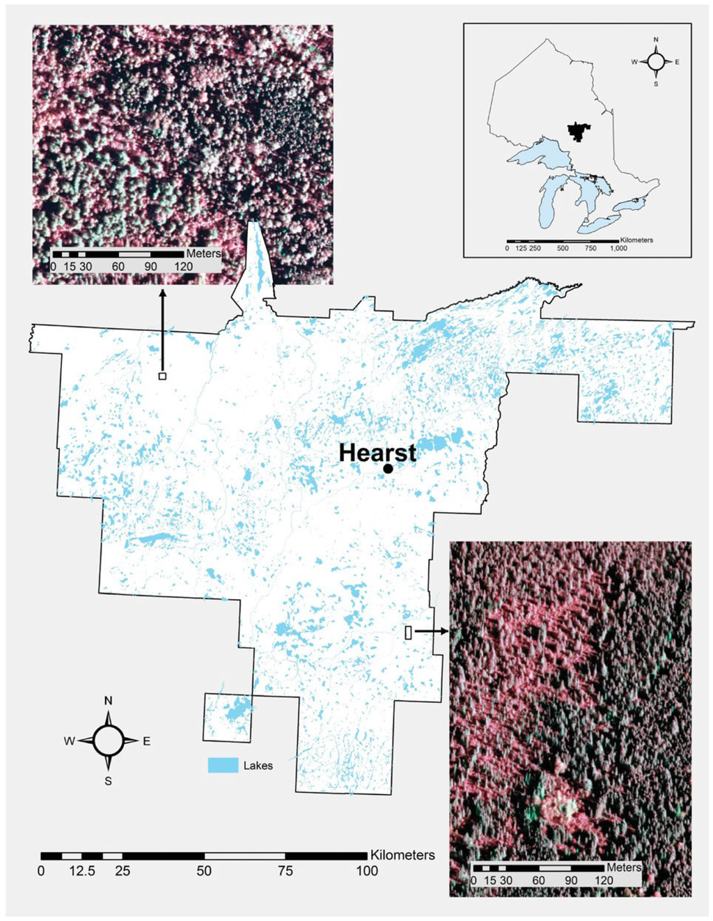
Figure 1.
The location of the Hearst Forest is given. Insets provide examples of the aerial imagery used in the study.
Figure 1.
The location of the Hearst Forest is given. Insets provide examples of the aerial imagery used in the study.


Table 1.
The forest types used in the analysis are described.
| Forest Type | Description |
|---|---|
| SB | Nearly pure black spruce growing on wet, deep organic soils |
| LC | Mixtures of black spruce, larch and/or cedar growing on wet, deep organic soils |
| PJ | Nearly pure stands of jack pine and mixed stands of jack pine/black spruce growing on dry to moist sandy to coarse loamy soils |
| SP | Upland black spruce on fresh to moist mineral soils |
| SF | Mixed conifer stands of white spruce, balsam fir, black spruce and cedar on fresh to moist mineral soils. |
| IH | Intolerant hardwoods dominated by poplar and/or white birch |
| MWC | Mixed conifer/hardwood stands with more conifer than hardwood |
| MWH | Mixed conifer/hardwood stands with more hardwood than conifer |
2.2. Ground (Field) Data
The majority of the ground data were collected on the Hearst Forest during the summer of 2010, according to a previously documented field protocol [2]. A total of 446 circular, 400-m2 temporary sample plots were established throughout the range of development stages within eight forest types (Table 1). As in prior analyses, four plots dominated by cedar with unusually high basal areas were not used. In late 2012, an additional 64 plots, eight in each forest type, were established using the same field protocol. A lower Dbh limit of 9 cm was used. Trees with Dbh > 9 cm were put into 2cm wide Dbh classes. Plots with three or fewer Dbh classes were withheld from analyses. Plots with less than 3 m2/ha of live basal area were also excluded, leaving a total of 401 plots. Veteran trees, defined as solitary, large trees that were significantly taller and older than the main canopy, were removed from the ground plot tallies.
The vertical complexity index (VCI) [21] was computed from the ALS data as a means of stratifying the ground plots within forest types. VCI summarizes the vertical distribution of the ALS returns on a scale of 0 to 1 and is computationally similar to the Shannon [22] evenness index, which is used to quantify species diversity and evenness. The index is at a maximum when the frequency distribution is a uniform distribution and decreases as the distribution becomes more peaked. In general, plots with smaller VCI tended to be in younger stands with a right-tailed Dbh distribution. As VCI increases, the distributions tend toward a more symmetric, unimodal distribution. As the VCI approaches 1, the distributions tend to flatten with no clear mode or multiple modes. Plots with high VCI tend to be associated with overmature conditions where the overstorey is starting to break up and an understorey is developing. The stratification is similar to that used by Bollandsås and Næsset [23] who used the Gini coefficient to group by distribution types, ranging from normal, to uniform, to reverse-J. Alternatives to VCI that better characterize forest structural types [24] are available. VCI was used here to ensure the validation data covered a range of conditions, not necessarily to identify forest structural types, and was felt to be adequate for this use.
Eight plots in each forest type, randomly selected throughout the range of VCI, were reserved for validation (Table 2 and Table 3).
Table 2.
The number of plots is given by forest type and vertical complexity index (VCI) class. The number of calibration plots is followed by the number of validation plots (in brackets).
| VCI Class | LC | MWC | MWH | PJ | IH | SB | SF | SP | Total |
|---|---|---|---|---|---|---|---|---|---|
| 0.3 | 1 (0) | 1 (0) | |||||||
| 0.4 | 1 (1) | 1 (1) | 2 (2) | ||||||
| 0.5 | 1 (0) | 1 (0) | 4 (1) | 8 (2) | 5 (1) | 3 (1) | 22 (5) | ||
| 0.6 | 8 (4) | 6 (2) | 5 (2) | 11 (3) | 17 (3) | 57 (3) | 20 (3) | 7 (2) | 131 (22) |
| 0.7 | 8 (4) | 16 (3) | 26 (4) | 11 (2) | 24 (4) | 37 (3) | 9 (2) | 17 (4) | 148 (26) |
| 0.8 | 8 (3) | 9 (2) | 8 (2) | 6 (1) | 1 (1) | 1 (0) | 33 (9) | ||
| Total | 17 (8) | 31 (8) | 40 (8) | 35 (8) | 47 (8) | 102 (8) | 36 (8) | 29 (8) | 337 (64) |
Table 3.
The ground plots are summarized by forest type (including the eight plots from each forest type that were reserved for validation). The mean is followed by the range (in brackets).
| Forest Type | N | Basal Area (m2/ha) | Total Stem Volume (m3/ha) | Top Height (m) | Quadratic Mean Dbh (cm) |
|---|---|---|---|---|---|
| LC | 25 | 38.4 (20.1–62.3) | 190 (67–380) | 15.5 (8.8–22.2) | 13.0 (6.2–23.2) |
| MWC | 39 | 29.1 (11.7–44.8) | 198 (43–338) | 19.3 (7.7–28.4) | 14.5 (5.8–31.8) |
| MWH | 48 | 29.0 (8.3–57.6) | 212 (44–520) | 19.8 (13.9–27.4) | 15.7 (7.7–26.1) |
| PJ | 43 | 28.6 (4.7–45.9) | 208 (24–401) | 17.4 (10.5–26.3) | 13.5 (6.9–23.5) |
| IH | 55 | 29.1 (10.0–55.3) | 230 (51–542) | 19.9 (13.4–28.9) | 15.5 (7.1–30.7) |
| SB | 110 | 28.9 (11.8–51.8) | 161 (53–366) | 15.5 (10.5–20.9) | 11.3 (5.3–20.2) |
| SF | 44 | 30.4 (10.8–50.0) | 162 (39–319) | 15.6 (8.6–24.6) | 11.9 (4.8–23.8) |
| SP | 37 | 31.6 (17.6–52.9) | 191 (60–363) | 17.0 (8.3–21.3) | 12.4 (6.0–19.5) |
2.3. ALS Data
The ALS data were acquired between 4 July and 4 September 2007 according to the specification provided in Table 4. ALS predictor variables were derived from point-cloud statistics (Table 5) following the methods described by Woods et al. [2].
Table 4.
The ALS specifications are given.
| Parameter | ALS | Aerial Imagery |
|---|---|---|
| Sensor | Leica ALS50 | Leica ADS40 |
| Platform | Cessna 310 | Cessna 310 |
| Pulse rate | 119,000 Hz | |
| Scan rate | 32 Hz | |
| Field of view | 30° | 42° |
| Flying height | 2,400 m | 2,400 m |
| Line spacing | 1,000 m | 3,000 m |
| Overlap | 20% | 30% (max) |
| Vertical accuracy | < 30 cm | |
| Pulse density | ~1.0/m2 | 2.4/m2 |
Table 5.
ALS and image point cloud predictor variables are defined. Field names with a “_95” ending are based on the lower 95% of returns.
| Field name | Description | ALS | IPC |
|---|---|---|---|
| MEAN | Mean height (m) | √ | √ |
| STD_DEV_95 | Standard deviation | √ | √ |
| ABS_DEV_95 | Absolute standard deviation | √ | √ |
| SKEW_95 | Skewness | √ | √ |
| KURTOSIS_95 | Kurtosis | √ | √ |
| P10 | First Decile ALS height (m) | √ | √ |
| P20 | Second Decile ALS height (m) | √ | √ |
| ↓ | ↓ | ↓ | |
| P80 | Eighth decile ALS height (m) | √ | √ |
| P90 | Ninth decile ALS height (m) | √ | √ |
| MAX | Maximum height (m) | ||
| D1 | Cumulative percentage of the number of returns found in bin 1 of 10 | √ | √ |
| D2 | Cumulative percentage of the number of returns found in bin 2 of 10 | √ | √ |
| ↓ | ↓ | ↓ | |
| D8 | Cumulative percentage of the number of returns found in bin 8 of 10 | √ | √ |
| D9 | Cumulative percentage of the number of returns found in bin 9 of 10 | √ | √ |
| DA_95 | First returns/ all returns | √ | |
| DV_95 | First vegetation returns/all returns | √ | √ |
| DB_95 | First and only return / all returns | √ | |
| VDR_95 | Vertical distribution ratio = [max−median]/max | √ | √ |
| Covar_95 | Std Dev (all returns)/ mean (all returns) | √ | |
| CanCovar_95 | Std Dev (first returns only)/ mean (first returns only) | √ | √ |
| VCI_95 | Vertical complexity index [ 20] | √ | √ |
| cc2 | Crown closure: the number of 2 m × 2 m canopy height model raster cells that have a height value greater or equal to 2 m divided by the number of nonvoid 2 m × 2 m cells, expressed as a percen t | √ | √ |
| ↓ | ↓ | ↓ | |
| cc26 | Crown closure: the number of 2 m × 2 m canopy height model raster cells that have a height value greater or equal to 26 m divided by the number of nonvoid 2 m × 2 m cells, expressed as a percen | √ | √ |
| cc28 | Crown closure: the number of 2 m × 2 m canopy height model raster cells that have a height value greater or equal to 28 m divided by the number of nonvoid 2 m × 2 m cells, expressed as a percen | √ | √ |
| TD2 | Cumulative percentage of vegetation returns 0-2m | √ | |
| TD4 | Cumulative percentage of vegetation returns 0-4m | √ | |
| ↓ | ↓ | ||
| TD30 | Cumulative percentage of vegetation returns 0-30m | √ | |
| s2 | % of vegetation returns in slice 0-2m | √ | |
| s4 | % of vegetation returns in slice 2-4m | √ | |
| ↓ | ↓ | ||
| s30 | % of vegetation returns in slice 28-30m | √ |
2.4. Image-Based Data
Aerial imagery for the Hearst Forest was acquired with the Leica ADS40 sensor during July and August 2007 as part of the provincial Forest Resources Inventory acquisition effort [25,26]. The data included stereo coverage with panchromatic, red, green, blue, and infrared bands, acquired at a ground sampling distance of 16 cm, and later resampled to 20 cm for the panchromatic and 35 cm for the 4-band multispectral data (Table 4; Figure 1). Photogrammetric pixel matching was completed by the image vendor, using the semi-global matching algorithm [27,28,29,30] on 80 cm resolution, 4-band multispectral data. The resulting IPC had an average sampling density of 2.4 pixel matches/m2 and described the surface captured on the image (ground, low vegetation, or trees), but were not classified as such. These IPCs were then normalized against the ALS-derived digital terrain model (DTM). Normalized IPC statistics and a digital canopy height model were generated for both datasets.
3. Methods
3.1. Dependent Variables
The prediction unit was the 400-m2 plot. The parametric dependent variable was relative basal area (BA), the fraction of total BA by 2-cm Dbh class on the 400-m2 plot. The choice of 2-cm wide Dbh classes was somewhat arbitrary. For the calibration data, it led to an average of 9 Dbh classes with trees present. The lower limit for Dbh was 9 cm; the lower limit considered for merchantability. The total BA per hectare, as well as the fraction of basal area in trees with Dbh > 9 cm, were predicted [31], and used herein to convert relative BA by Dbh class to BA by Dbh class.
The nonparametric dependent variable was the BA/ha by Dbh class on the 400-m2 plot. We considered predicting the relative BA by Dbh class, but these predictions would have required scaling to ensure that they summed to one. Since both the relative BA and the absolute BA would require scaling, it was decided to select the raw BA for modeling. These BA predictions were then converted to relative BA by dividing the BA by Dbh class by the sum of the predicted BA by Dbh class. Parametric and nonparametric predictions of relative BA were then compared.
3.2. Independent ALS and Optical CHM Predictors
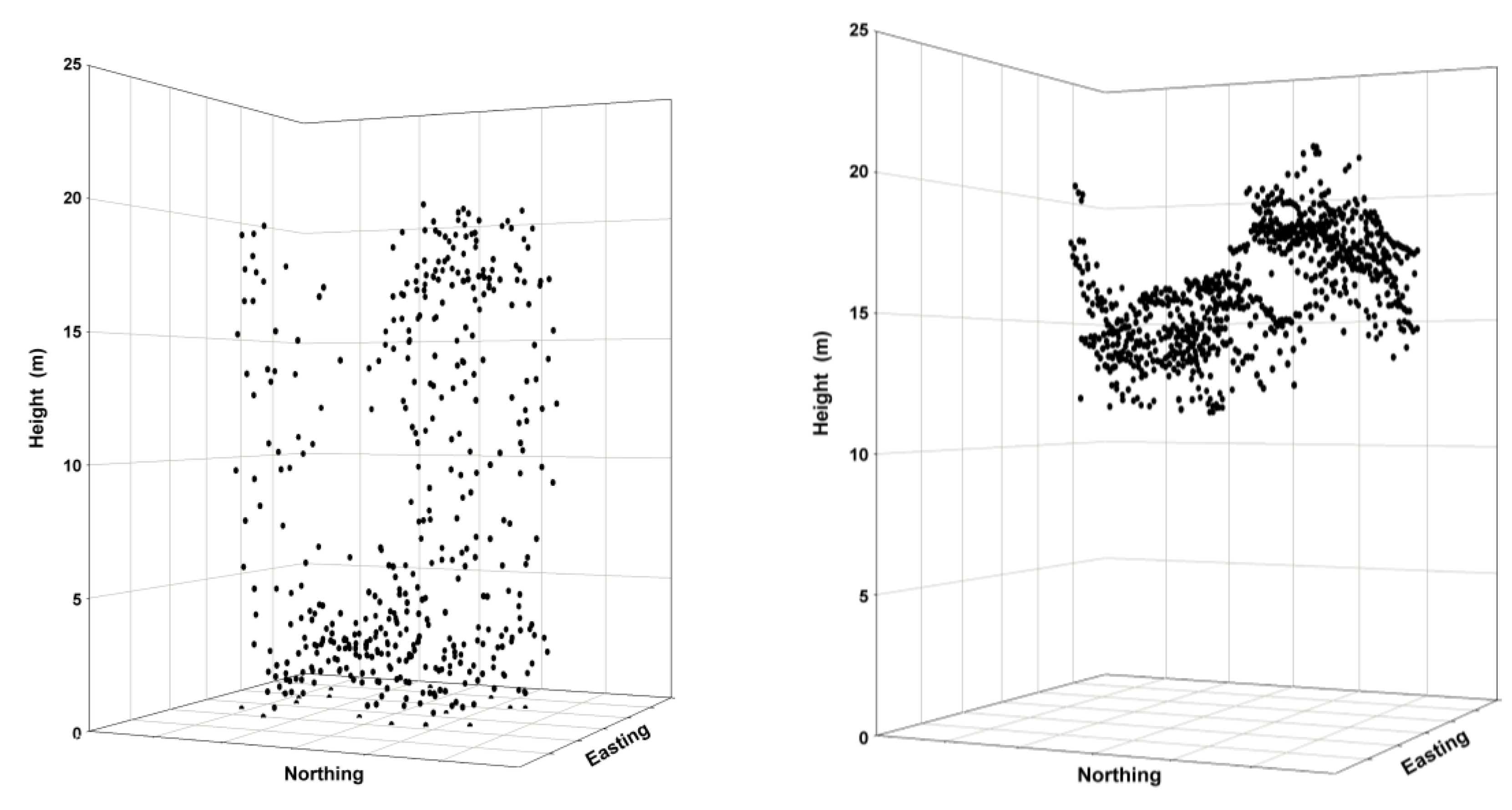
Both the ALS and IPC data require normalization against a DTM. The IPC point cloud is concentrated in the upper canopy envelope, compared to the ALS point cloud, which is distributed throughout the canopy (Figure 2). The better canopy penetration of ALS makes it much more suitable to the generation of a DTM [32] in a forested environment. For this study, a DTM was generated from the ALS data and the ALS and IPC data were normalized against this DTM.
The ALS predictor variables (Table 5) were derived from point-cloud statistics following previously described methods [2]. Veteran trees generally result in a few high ALS returns that have a large influence on some of the measures of spread, such as standard deviation of ALS returns (STD_DEV) and vertical complexity index (VCI). To reduce the influence of these trees on measures of spread, these statistics were calculated by first removing the top 5% of the ALS returns, and basing the statistic on the remaining 95% of returns. The remaining statistics were calculated using all ALS returns.
The IPC data were intersected with the ground plots and independent predictors were generated (Table 5). Not all statistics generated with the ALS point clouds were generated from the IPC. Exceptions were the statistics that are dependent on ratios of the number of points distributed through the canopy (first return divided by all returns [DA], first and only return/all returns [DB], and coefficient of variation [CanCovar]), which could not be calculated for the IPC data.

Figure 2.
Point clouds are illustrated as three-dimensional plots for a sample 400-m2 forested plot (ALS left panel; IPC right panel). ALS returns are distributed throughout the canopy and include the forest floor. In contrast, IPC elevation measures exist only for features shown on the image—in this case, the canopy surface. If a quality DTM exists, then the IPC-derived canopy surface measures can be translated into actual height values.
3.3. Parametric or Non-Linear Regression (NLS)
The choice of a 2-cm diameter class interval meant that some Dbh classes had no trees. These could either be treated as missing observations, and not used in the statistical analysis, or as zeroes, and used in the statistical analysis. In this study, we chose to set missing values to 0 for Dbh classes within the range of Dbhs for the plot. For example, if the Dbh range for a plot went from 10 to 32 cm, any Dbh classes within that interval with no trees had zero trees (no missing values). We set the relative frequency one size larger than the largest Dbh to zero as well. The result was that missing values were only allowed for Dbh classes > the largest Dbh class + 2 cm.
Our methods draw heavily from Cao [6], who used the three-parameter Weibull (Equation (1)) to model Dbh distributions. The Weibull probability density function predicts the relative frequency of x, given location parameter “a”, shape parameter “b”, and scale parameter “c”.
where
We used the parameter prediction method [6]. First, we fit Equation (1) to each calibration plot using PROC NLIN in SAS, with a = 9.0. Then we used stepwise regression (SAS routine GLMSELECT) to predict the parameters of the plot-level fit from ALS or IPC attributes by forest type. We used a logarithmic transformation to ensure the parameter predictions were always positive. We predicted the natural logarithm of the shape parameter (ln(b)) and the scale parameter (ln(c)) as linear combinations of the natural logarithm of the predictor variables (X1 .. Xp-1) from Table 5. The coefficients b11 … b2p are estimated parameters.
Next, we fit the original model as a single equation expressing the difference between two cumulative density functions (F(x)), with the location parameter a set to 9.0 cm. We removed non-statistically significant (probability < 0.05) parameters from the model.
Model (3) was fit by forest type.
3.4. Non Parametric or RandomForest Nearest Neighbour Prediction
We used nearest neighbour methods [11] to impute the size class distributions for the target prediction units. The distance measure to identify nearest neighbours was calculated using randomForest and the predictions are referred to as randomForest Nearest Neighbour (RFNN). RandomForest [33] is a nonparametric technique that generates a “forest” of regression trees. Each regression tree is grown using binary partitioning so that at each node, the training data are split into two groups using a single predictor. This binary partitioning continues until each final group (“node” or “leaf”) contains a user-specified number of data points. Each tree is grown with a random subset of the training data and the decision variable at each node is drawn from a random subset of the potential predictor variables. The distance between a target prediction unit and each point in the reference data set is one minus the proportion of trees where the target prediction unit is in the same terminal node as the reference observation.
The R package yaImpute [34] was used identify the nearest neighbour (k = 1) in the reference dataset which was then used to impute the array of BA by 2 cm Dbh class, ranging from Dbh9, Dbh11, …, Dbh69 where Dbhi is the Dbh class (i – 1) ≤ Dbh < (i + 1). The function “yai” was used with method = “randomForest” and the supplied defaults, including the number of regression trees = 500 and mtry (the number of predictor variables picked a random) equal to the square root of the number of predictor variables. Unlike the parametric predictions, the data were not stratified by forest type.
3.5. Evaluating Fit
The predictions were evaluated by visually comparing the predicted and observed distributions as well as two measures of fit.
The first measure of fit was the index developed by Reynolds et al. [34], which was used to measure the closeness of Dbh predictions to the data. Let be the cumulative density function (cdf) of diameters (x) on a plot predicted by the model and be the observed cdf. Let w(x) be a weight function and N the number of trees/ha. The Reynolds error index is the following.
Reynolds et al. [35] suggested setting the weight to the volume of a tree in diameter class x or the dollar value of the tree. We set the weight to the basal area of a tree with Dbh x. The error index was calculated as the weighted absolute differences in frequencies summed over all diameter classes:
The statistical properties of the index are unknown but the smaller the index, the better the agreement between the predicted and observed distribution.
A second measure of fit was the closeness of the quadratic mean diameter (DQ) calculated from the predicted distribution compared to the actual DQ. This measure is relatively insensitive to the shape of the distribution.
Our 400 m2 prediction unit is relatively small, resulting in some jagged Dbh distributions (e.g., Figure 3c). Moreover, graphical summaries have limited usefulness when plots contain a relatively small (<40) number of trees [9]. Larger plots or areas of prediction, such as stands or blocks, may be expected to have smoother distributions. Therefore, we grouped validation plots by forest type as well as VCI class, a measure of the entropy of the vertical distribution of the ALS returns, to better assess prediction results.
The error index and DQ prediction errors were subjected to repeated measures analysis of variance. In this study, four error indices and four DQ prediction errors were calculated for each plot corresponding to two remote sensing methods (IPC vs. ALS) and two prediction methods (SUR vs. RFNN). The following hypotheses were tested.
- H0: ALS = IPC. The error index does not depend on remote sensing technique (ALS vs. IPC).
- H1: ALS ≠ IPC. The error index depends on remote sensing technique (ALS vs. IPC).
- and
- H0: SUR = RFNN. The error index does not depend on statistical technique (SUR vs. RFNN).
- H1: SUR ≠ RFNN. The error index depends on statistical technique (SUR vs. RFNN).
As well, the interaction between remote sensing and statistical technique was tested. Similar hypotheses were tested for DQ prediction errors. Forest type was included as a fixed-effect, blocking variable.
4. Results
4.1. Parametric Predictions
The parametric predictions of relative BA were converted to BA (m2/ha) by diameter class using the prediction equations developed in [31] to predict total BA and the proportion of BA in trees with Dbh > 9.0 cm. We found that the results were sensitive to the size of the Dbh class interval and the size uniformity of the trees on the sample plots. Single-storey, even-aged stands could generally be well represented with a unimodal distribution (Figure 3a). With a prediction unit as small as 400 m2, size distributions were often not unimodal, particularly with small (2-cm wide) Dbh classes, and were poorly predicted with a Weibull function (Figure 3b). If wider Dbh class intervals were used, it is possible that the plot in Figure 3b would resemble a uniform distribution. Figure 3c is an example of a possible two-storied stand. These sample distributions illustrate one of the difficulties of parametric prediction—the parametric approach to predicting distributions is limited by the capability of the distribution function to adequately represent the true distribution. Part of this is due to the relatively small plot size used, but the complexity of the tree size distributions also has an impact.
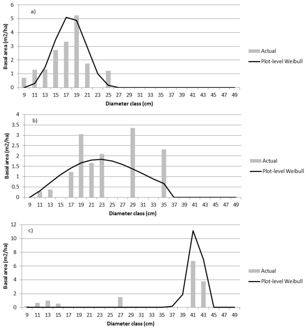
Figure 3.
The actual size class distributions are compared to predictions using Equation (1) for three sample plots—plot 34 (a), plot 6 (b), and plot 44 (c). The dependent variable is the relative proportion of BA within each diameter class.
Figure 3.
The actual size class distributions are compared to predictions using Equation (1) for three sample plots—plot 34 (a), plot 6 (b), and plot 44 (c). The dependent variable is the relative proportion of BA within each diameter class.

The variables selected by stepwise regression (Equation (2)) varied by forest type, resulting in final parametric models that varied by these strata. The ALS and IPC predictions were similar and reasonably close to the actual distribution for unimodal distributions (Figure 4a). The prediction of more complex distributions was less satisfactory (Figure 4b,c). For the ALS-based predictions, one or more of VDR_95, VCI_95, and p90 appeared in each model except in the LC forest type. For the IPC-based predictions, CC values, particularly CC2, CC14, and CC16 occurred in most models. There was more similarity in predictors across strata within data sources (ALS vs. IPC) than across data sources for the same stratum. A concern of the parametric modeling approach was the overestimation of basal area in the larger Dbh classes as the model form tries to smoothly feather the basal area distribution.
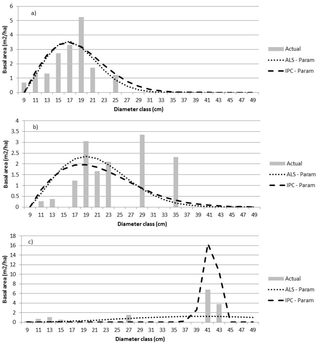
Figure 4.
The actual size class distributions are compared to predictions using Equation (1) for three sample plots—plot 34 (a), plot 6 (b), and plot 44 (c). The dependent variable is the relative proportion of BA by diameter class. The error indices for a) are 1.76 (ALS) and 1.61 (IPC); for b) are 3.88 (ALS) and 3.18 (IPC); and for c) are 1.43 (ALS) and 1.78 (IPC). Parametric predictions have been converted to BA by Dbh class to permit comparisons.

4.2. Nonparametric Predictions
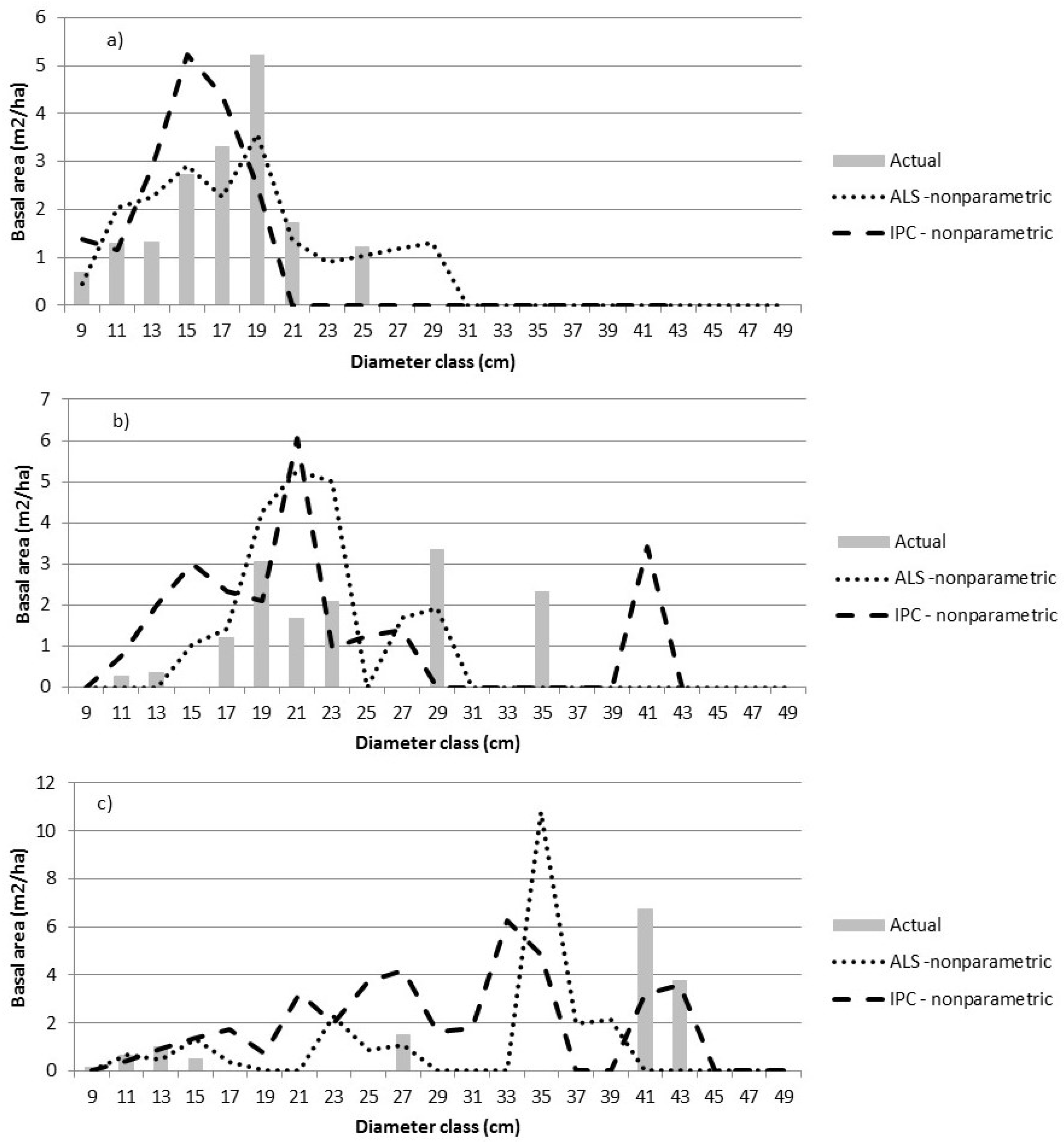
The nonparametric predictions were more irregular than the parametric predictions (Figure 5). RFNN essentially looks for nearest neighbours in the reference dataset in terms of the ALS predictor attributes (P40, d10, etc.). The reference dataset did not appear to be large enough to find close neighbours for all the observed size-classes (e.g., Figure 5b) but, in contrast to the parametric modeling approach, the nonparametric models were able to predict multi-modal distributions. In addition, the nonparametric models do not predict tree sizes outside the range in the reference data set. The imputations here come from the single nearest neighbour (k = 1), resulting in jagged distributions. The number of neighbours used could be increased and weighted by the distance from the target observation. This would likely result in smoother distributions. We used a single nearest neighbour, resulting in a realistic, jagged distribution at the plot level. When the imputations from the individual prediction units are aggregated to a stand or block, the resulting distribution will be smoother.
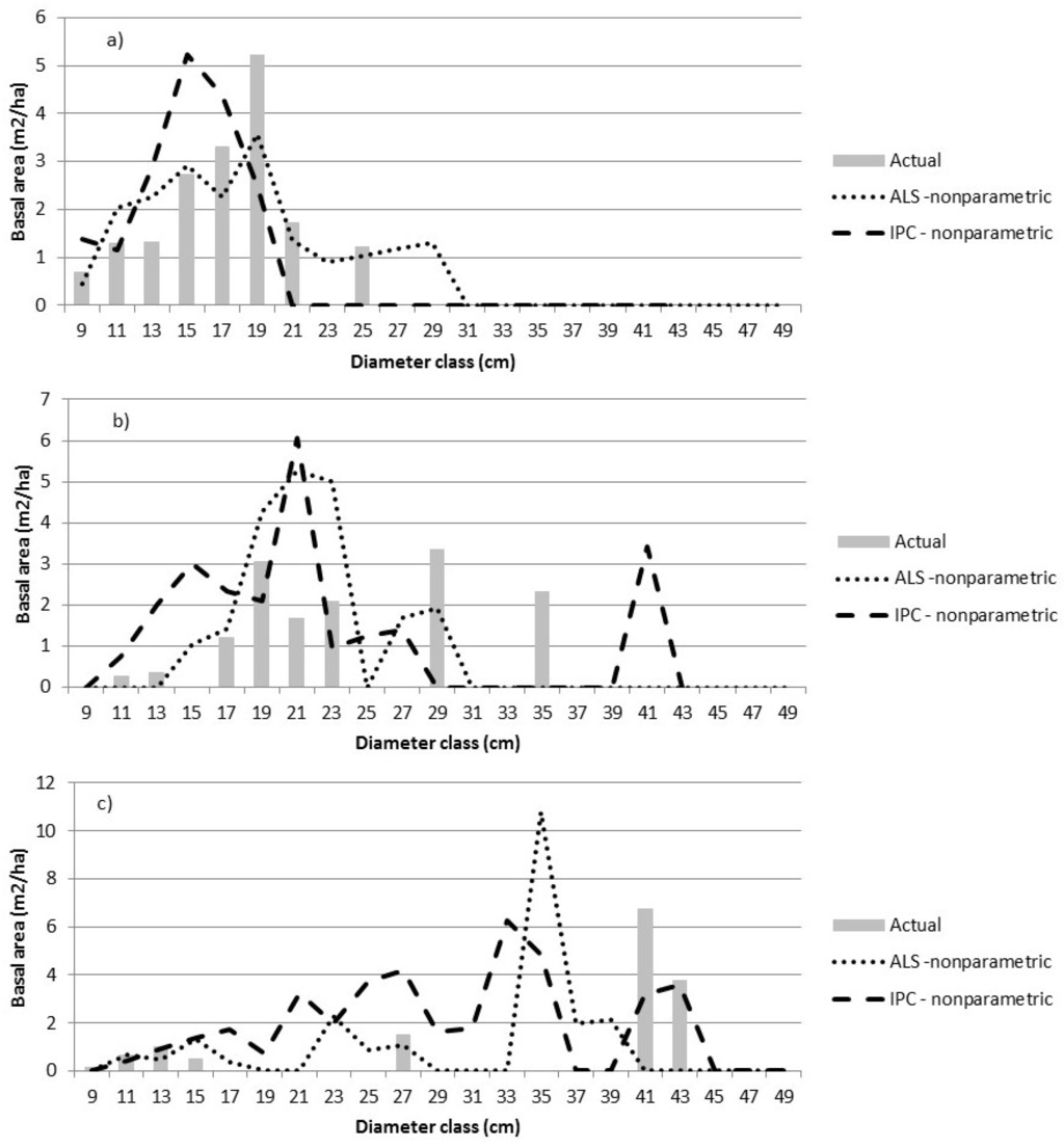
Figure 5.
The actual size class distributions are compared to nonparametric predictions for three sample plots—plot 34 (a), plot 6 (b), and plot 44 (c). The dependent variable is the relative proportion of BA by diameter class. The error indices for a) are 1.45 (ALS) and 1.90 (IPC); for b) are 2.94 (ALS) and 3.78 (IPC); and for c) are 1.98 (ALS) and 1.98 (IPC).
The differences between the ALS and IPC nonparametric predictions were greater than those observed for the parametric predictions. When validation plots were grouped by VCI class (i.e., representing an area larger than 400 m2), the actual distributions were smoother and the ALS and IPC parametric predictions were very close (Figure 6).
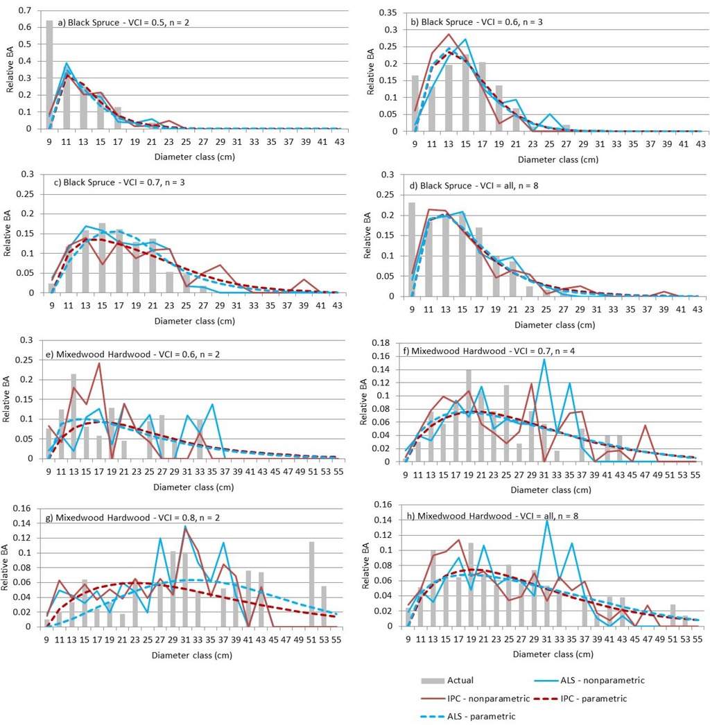
Figure 6.
Parametric and nonparametric relative basal area by diameter class results are given for the black spruce and mixed hardwood validation plots aggregated by VCI class.
Figure 6.
Parametric and nonparametric relative basal area by diameter class results are given for the black spruce and mixed hardwood validation plots aggregated by VCI class.
4.3. Measures of Fit
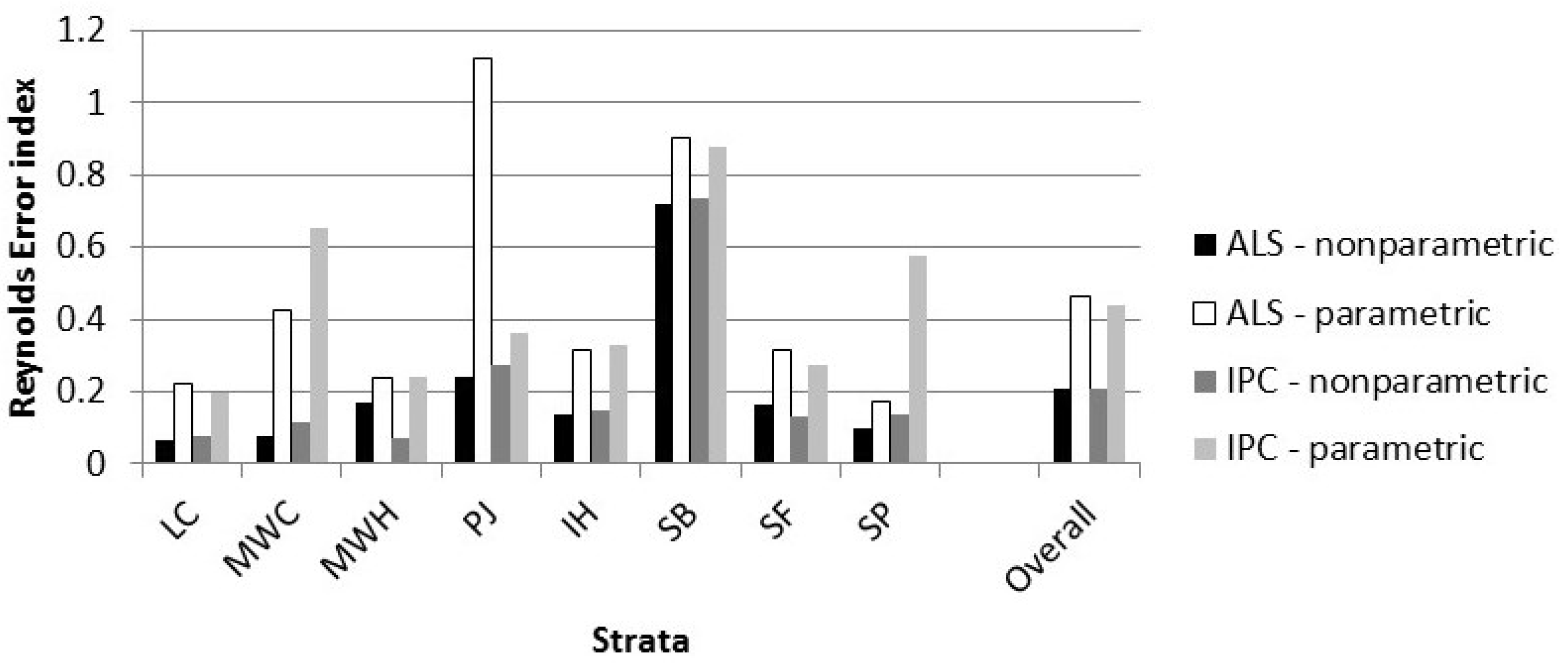
The error index was computed using 2-cm Dbh intervals. The smaller the index, the better the agreement between the actual and observed distribution. The differences in error index were small and within the range of variation within the strata. Again, the plot size, 400-m2, is small for estimating meaningful size class distributions. Predictions are expected to perform better when prediction units are aggregated over a larger range, for example, at the stand polygon or harvest block level. Results from accuracy assessments vary with the scale (in terms of area), of the assessment [36]. Therefore, the error indices were also calculated after combining all the validation plots within a stratum (Figure 7).

Figure 7.
The strata level error index is given for the validation data. All the plots within a stratum were combined prior to calculating the index.
Figure 7.
The strata level error index is given for the validation data. All the plots within a stratum were combined prior to calculating the index.
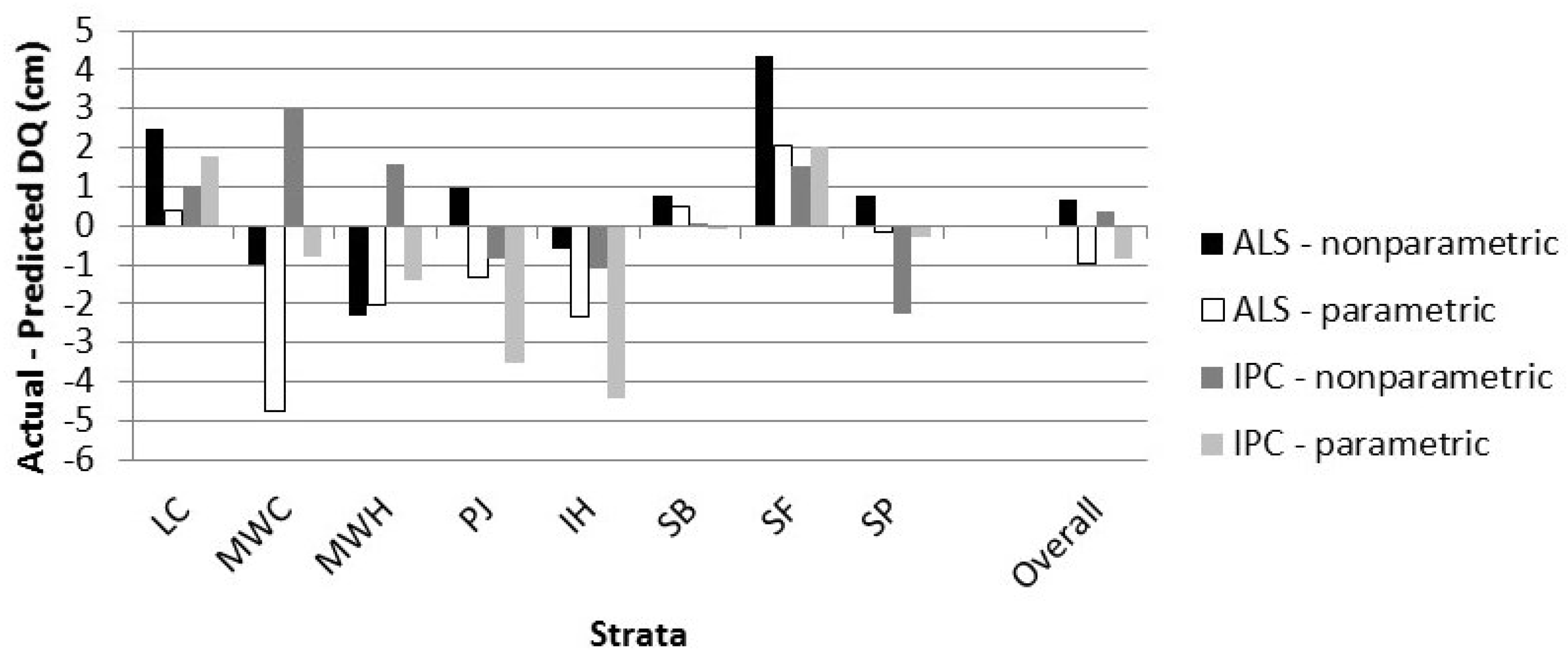
We obtained similar results when comparing the actual DQ to the DQ calculated from the predicted Dbh distribution (Figure 8). The DQ errors for lowland black spruce (SB) were particularly small, due in part to the smaller DQ. For nonparametric predictions, the average bias, when calculated at the plot level, was larger than when the bias was calculated by strata. The opposite was true for the parametric predictions.

Figure 8.
The average difference between the DQ calculated from the actual distribution and the DQ calculated from the predicted size class distribution. The difference is given for the validation data, averaged by strata. All the plots within a stratum were combined prior to calculating the bias.
Figure 8.
The average difference between the DQ calculated from the actual distribution and the DQ calculated from the predicted size class distribution. The difference is given for the validation data, averaged by strata. All the plots within a stratum were combined prior to calculating the bias.
In general, the nonparametric predictions were marginally better (lower error index) than the parametric predictions. The differences between the ALS and IPC predictions were smaller. The largest error indices were associated with lowland black spruce (SB), the forest type with the most samples, but a relatively small average tree size.
Repeated measures analysis of variance results show statistically significant differences between statistical techniques (p = 0.0145) but not between remote sensing techniques or forest types (p ≥ 0.1812) for DQ error (Table 6). For the error index, there are statistically significant differences by forest type and for statistical technique (p ≤ 0.0199) but not by remote sensing technique (p = 0.6048).
Table 6.
The repeated measure analysis of variance results are given. The probability that the null hypothesis (H0) is supported by the data is given. Statistically significant differences (probability < 0.05) are shaded.
| Error Index | Error Index | DQ Error | |
|---|---|---|---|
| Remote sensing technique (RS) | H0: ALS = IPC | 0.6048 | 0.8096 |
| H0: no forest type effect | 0.0449 | 0.4541 | |
| Statistical technique (S) | H0: SUR = RFNN | <0.0001 | 0.0145 |
| H0: no forest type effect | 0.3161 | 0.3770 | |
| RS x S interaction | H0: no interaction | 0.6128 | 0.8660 |
| H0: no forest type effect | 0.0199 | 0.1812 |
5. Discussion
The differences between the ALS and IPC predictions are minor and not statistically significant when compared in terms of error index or DQ. Comparable results for ALS and IPC suggest that the choice of remote sensing can be based on other considerations. If an appropriate quality DTM is not available, IPC is not a viable option because the point cloud requires such a DTM for normalization. If a DTM is available, IPC may be the preferred method, since the point-cloud data may be generated at minimal additional cost when the same imagery is required for species interpretation to support inventory work.
The differences between parametric and nonparametric predictions when compared in terms of error index and DQ were statistically significant. Agreement between the actual and predicted size class distributions was poor for some plots, due in part to the small prediction unit size and relatively narrow Dbh class width used. Ground sampling is expensive and plot size is generally balanced by the number of samples. Prediction unit size is a function of the spatial resolution desired for the inventory attributes, and ~400 m2 has been found to be a suitable size for both ALS [2] and IPC [3] predictions in the boreal forest. Larger prediction units may be used, but as the size increases, so does the cost of calibration and validation. Decisions regarding Dbh class width can affect parametric estimates. However, the resulting models can be used to predict the relative BA for any Dbh interval. In contrast, nonparametric imputation is tied to the Dbh class width associated with the training data—classes can be aggregated but not split. The inflexibility of the nonparametric predictions with respect to Dbh class width led to the choice of a relatively narrow Dbh class width. Alternatively, broader Dbh classes could have been used and finer intervals could be interpolated from the nonparametric predictions.
Parametric distributions have positive relative frequencies for all positive diameters, creating the need to truncate the right side of the distribution to avoid the over-estimation of BA into larger Dbh classes. Several options exist, including predicting the maximum Dbh for each pixel, setting relative frequencies below some threshold to zero, and capping predictions at the maximum observed Dbh in the calibration data. Parametric predictions often benefit from stratification into similar forest types, which can increase modeling costs. Nonparametric imputations generally use reference observations that are close or similar by some measure, obviating the need for stratification.
BA (m2/ha) by Dbh class, rather than relative BA by Dbh class, is generally of interest. For the parametric models, this requires a prediction of total BA in trees larger than the minimum Dbh. For this study, those predictions were developed earlier [31]. The error index and DQ used here to evaluate the predictions used relative BA.
This study deliberately focused on merchantable-sized trees (Dbh > 9.0 cm). Small errors in the BA associated with small trees can lead to unreasonably large estimates of stems/ha. A previous study [31] derived estimates of total BA and the relative BA in merchantable-sized trees. The BA in smaller trees can thus be estimated. It could also be partitioned into size classes, but we have found that error rates are high.
Diameter distribution predictions are best suited to aggregates of prediction units (e.g., stands or other areas of interest), which complicates validation since the spatial definition and measurement of large plots on the ground can be difficult and prohibitively expensive. In this study, we attempted to get around this obstacle by aggregating and validating predictions by forest type or VCI class. Recent advancements in harvesting equipment (e.g., MultiDatTM data loggers, [37]) allow the measurement and recording of the stem diameter (and many other parameters, including stem taper and product volume) of each tree as it is harvested, presenting the best opportunity for validating inventory predictions.
Alternatively, a tree-based approach can be used. First, tree crowns are delineated using ALS [38], and Dbh is estimated from the tree crowns [39]. The relative accuracies of tree-based and area-based estimates vary, depending on the attribute [40] and the degree to which crowns are visible from above, leading to research into combining tree- and area-based approaches (e.g., [41]).
6. Conclusions
Area-based forest inventories have been developed using ALS metrics and generally include estimates of per hectare values (BA, volumes, etc.) as well as mean tree attributes (e.g., DQ). Tree-based ALS inventories contain much desired information on individual tree dimensions. The addition of size class distributions to area-based inventories bridges some of the gap between area- and tree-based inventories. This study examined the potential of ALS and IPC to predict size class distributions in a boreal forest. Given an accurate digital terrain model, both ALS and digital stereo aerial photos provide size class distributions that were not statistically different in terms of error index and DQ error. Nonparametric imputations were associated with lower error index and DQ error values than parametric imputations. This may be related to the limitation of using a unimodal Weibull function on a relatively small prediction unit size. Generally, it is expected that predictions based on aggregated prediction units will perform better than comparisons on a single prediction unit.
Acknowledgments
We are greatly indebted to Hearst Forest Management Inc. for access to the ALS data and to Dave Nesbitt (Ontario Ministry of Natural Resources and Forestry) for his data processing prowess. Financial and in-kind resources for the research introduced in this paper were provided by the Canadian Wood Fibre Centre of the Canadian Forest Service, and the Ontario Ministry of Natural Resources and Forestry. Finally, special thanks to Karen Jamieson, Kate Johnson, and three anonymous reviewers for thorough and excellent reviews of earlier versions of this manuscript.
Conflict of Interest
The authors declare no conflict of interest.
References
- Næsset, E. Estimating timber volume of forest stands using airborne laser scanner data. Remote Sens. Environ. 1997, 61, 246–253. [Google Scholar] [CrossRef]
- Woods, M.; Pitt, D.; Lim, K.; Nesbitt, D.; Etheridge, D.; Penner, M.; Treitz, P. Operational implementation of a LiDAR inventory in Boreal Ontario. For. Chron. 2011, 87, 512–528. [Google Scholar] [CrossRef]
- Pitt, D.G.; Woods, M.; Penner, M. A comparison of point clouds derived from stereo imagery and airborne laser scanning for the area-based estimation of forest inventory attributes in boreal Ontario. Can. J. Rem. Sen. 2014, 40, 214–232. [Google Scholar] [CrossRef]
- Bailey, R.L.; Dell, T.R. Quantifying diameter distributions with the Weibull function. For. Sci. 1973, 19, 97–103. [Google Scholar]
- Thomas, V.; Oliver, R.D.; Lim, K.; Woods, M. LiDAR and Weibull modeling of diameter and basal area. For. Chron. 2008, 84, 866–875. [Google Scholar] [CrossRef]
- Cao, Q.V. Predicting parameters of a Weibull function for modeling diameter distribution. For. Sci. 2004, 50, 682–685. [Google Scholar]
- Kangas, A.; Maltamo, M. Calibrating predicted diameter distribution with additional information. For. Sci. 2010, 46, 390–396. [Google Scholar]
- Breidenbach, J.; Gläser, C.; Schmidt, M. Estimation of bivariate diameter and height distributions using ALS. In SilviLaser 2008: 8th International Conference on LiDAR: Applications in forest assessment and inventory, Heriot-Watt University, Edinburgh, UK, 17–19 September 2008; pp. 366–372.
- Magnussen, S.; Næsset, E.; Gobakken, T. Prediction of tree size distributions and inventory variables from cumulants of canopy height distributions. Forestry 2013, 86, 583–595. [Google Scholar] [CrossRef]
- McRoberts, R. Estimating forest attribute parameters for small areas using nearest neighbours techniques. Fore. Ecol. Mgmt. 2012, 272, 3–12. [Google Scholar] [CrossRef]
- Eskelson, B.N.I.; Temesgen, H.; LeMay, V.; Barrett, T.; Crookston, N.; Hudak, A. The roles of nearest neighbour methods in imputing missing data in forest inventory and monitoring databases. Scand. J. For. Res. 2009, 24, 235–234. [Google Scholar] [CrossRef]
- Temesgen, H.; LeMay, V.; Froese, K.; Marshall, P. Imputing tree-lists from aerial attributes for complex stands of south-eastern British Columbia. For. Ecol. Mgmt. 2003, 177, 277–285. [Google Scholar] [CrossRef]
- Guindon, L.; Ung, C.-H.; Beaudoin, A.; Miranda, M.; Villemaire, P.; Patry, A. Predicting stand table in a mixed forest of southern Quebec with airborne LiDAR using the kNN method. In Proceedings of the IUFRO Conference on Extending Forest Inventory and Monitoring over Space and Time, Quebec City, Canada, 19–22 May 2009; p. 5.
- Hudak, A.; Crookston, N.; Evans, J.; Hall, D.; Fallowski, M. Nearest neighbour imputation of species-level, plot-scale forest structure attributes from LiDAR data. Remo. Sens. Environ. 2008, 112, 2232–2245. [Google Scholar] [CrossRef]
- Magnussen, S.; Eggermont, P.; LaRiccia, V.N. Recovering Tree Heights from Airborne Laser Scanner Data. For. Sci. 1999, 45, 407–422. [Google Scholar]
- Mehtätalo, L.; Nyblom, J. Estimating Forest Attributes Using Observations of Canopy Height: A Model-Based Approach. For. Sci. 2009, 55, 411–422. [Google Scholar]
- Mehtätalo, L.; Nyblom, J. A Model-Based Approach for Airborne Laser Scanning Inventory: Application for Square Grid Spatial Pattern. For. Sci. 2012, 58, 106–118. [Google Scholar] [CrossRef]
- Bollandsås, O.; Maltamo, M.; Gobakken, T.; Naesset, E. Comparing parametric and non-parametric modelling of diameter distributions on independent data using airborne laser scanning in a boreal conifer forest. Forestry 2013, 86, 493–501. [Google Scholar] [CrossRef]
- Packalén, P.; Maltamo, M. Estimation of species-specific diameter distributions using airborne laser scanning and aerial photographs. Can. J. For. Res. 2008, 38, 1750–1760. [Google Scholar] [CrossRef]
- Hearst Forest Management Inc. Forest Management Plan for the Hearst Forest. Available online: http://www.hearstforest.com/english/PDF/HearstForest2007FMP.pdf (accessed on 3 November 2015).
- Van Ewijk, K.Y.; Treitz, P.M.; Scott, N.A. Characterizing forest succession in central Ontario using Lidar-derived indices. Photogramm. Eng. Rem. Sens. 2011, 77, 261–269. [Google Scholar] [CrossRef]
- Shannon, C.E. The mathematical theory of communication. Bell Syst. Tech. J. 1948, 27, 379–423. [Google Scholar] [CrossRef]
- Bollandsås, O.; Naesset, E. Estimating percentile-based diameter distributions in uneven-sized Norway spruce stands using airborne laser scanner data. Scan. J. For. Res. 2007, 22, 33–47. [Google Scholar] [CrossRef]
- Valbuena, R.; Packalen, P.; Mehtätalo, L.; Garcia-Abril, A.; Maltamo, M. Characterizing forest structural types and shelterwood dynamics from Lorenz-based indicators predicted by airborne laser scanning. Can. J. For. Res. 2013, 43, 1063–1074. [Google Scholar] [CrossRef]
- Ontario Ministry of Natural Resources. Ontario Forest Resources Inventory Calibration Plot Specifications—Revised; Ontario Ministry of Natural Resources Internal Publication: Ontario, Canada, 2012; p. 41. [Google Scholar]
- Ontario Ministry of Natural Resources. Ontario Forest Resources Inventory Photo Interpretation Specifications—Revised; Ontario Ministry of Natural Resources Internal Publication: Ontario Canada, 2012; p. 87. [Google Scholar]
- Hirschmüller, H. Stereo processing by semiglobal matching and mutual information. IEEE T. Pattern Anal. Mach. Intell. 2008, 30, 328–341. [Google Scholar] [CrossRef] [PubMed]
- Gehrke, S.; Morin, K.; Downey, M.; Boehrer, N.; Fuchs, T. Semi-Global matching: An alternative to LiDAR for DSM generation? Int. Arch. Photogramm. Remote Sens. 2010, 38. Part B1. [Google Scholar]
- Gehrke, S.; Uebbing, R.; Downey, M.; Morin, K. Creating and using very high density point clouds derived from ADS imagery. In Proceedings of the American Society of Photogrammetry and Remote Sensing 2011 Annual Conference, Milwaukee, WI, USA, 1–5 May 2011.
- Gehrke, S.; Downey, M.; Uebbing, R.; Welter, J.; LaRocque, W. A multi-sensor approach to semi-global matching. In International Archives of the Photogrammetry, Remote Sensing and Spatial Information Sciences, 2012 XXII ISPRS Congress, Melbourne, Australia, 25 August–1 September 2012; XXXIX-B3, pp. 17–22.
- Penner, M.; Pitt, D.G.; Woods, M.E. Parametric vs nonparametric LiDAR models for operational forest inventory in boreal Ontario. Can. J. Rem. Sens. 2013, 39, 426–443. [Google Scholar]
- Kraus, K.; Pfeifer, N. Determination of terrain models in wooded areas with airborne laser scanner data. ISPRS J. Photogramm. Remote Sens. 1998, 53, 193–203. [Google Scholar] [CrossRef]
- Liaw, A.; Wiener, M. Classification and Regression by randomForest. R News 2002, 2, 18–22. [Google Scholar]
- Crookston, N.I.; Finley, A.O. Yaimpute: An R package for kNN imputation. J. Stat. Softw. 2008, 23, 1–16. [Google Scholar] [CrossRef]
- Reynolds, M.R., Jr.; Burk, T.E.; Huang, W.-C. Goodness-of-fit tests and model selection procedures for diameter distribution models. For. Sci. 1988, 34, 373–399. [Google Scholar]
- Reichmann, R.; Wilson, B.; Lister, A.; Parks, S. An effective assessment protocol for continuous geospatial datasets of forest characteristics using USFS Forest Inventory and Analysis (FIA) data. Rem. Sens. Environ. 2010, 114, 2337–2353. [Google Scholar] [CrossRef]
- MultiDatTM. Available online: http://www.castonguay.biz (accessed on 15 July 2015).
- Leckie, D.; Gougeon, F.; Hill, D.; Quinn, R.; Armstrong, L.; Shreenan, R. Combined high-density lidar and multispectral imagery for individual tree crown analysis. Can. J. Rem. Sens. 2003, 20, 633–649. [Google Scholar] [CrossRef]
- Salas, C.; Ene, L.; Gregoire, T.G.; Næsset, E.; Gobakken, T. Modelling tree diameter from airborne laser scanning derived variable: A comparison of spatial statistical models. Remote Sens. Environ. 2010, 114, 1277–1285. [Google Scholar] [CrossRef]
- Peuhkurinen, J.; Mehtätalo, L.; Maltamo, M. Comparing individual tree detection and the area-based statistical approach for the retrieval of forest stand characteristics using airborne laser scanning in scots pine stands. Can. J. For. Res. 2011, 41, 583–598. [Google Scholar] [CrossRef]
- Xu, Q.; Hou, Z.; Maltamo, M.; Tokola, T. Calibration of area based diameter distribution with individual tree based diameter estimates using airborne laser scanning. IPRS J. Photogramm. Remote Sens. 2014, 93, 65–76. [Google Scholar] [CrossRef]
© 2015 by the authors; licensee MDPI, Basel, Switzerland. This article is an open access article distributed under the terms and conditions of the Creative Commons Attribution license (http://creativecommons.org/licenses/by/4.0/).