Analysis and Prediction of the IPv6 Traffic over Campus Networks in Shanghai

Abstract

With the exhaustion of IPv4 addresses, research on the adoption, deployment, and prediction of IPv6 networks becomes more and more significant. This paper analyzes the IPv6 traffic of two campus networks in Shanghai, China. We first conduct a series of analyses for the traffic patterns and uncover weekday/weekend patterns, the self-similarity phenomenon, and the correlation between IPv6 and IPv4 traffic. On weekends, traffic usage is smaller than on weekdays, but the distribution does not change much. We find that the self-similarity of IPv4 traffic is close to that of IPv6 traffic, and there is a strong positive correlation between IPv6 traffic and IPv4 traffic. Based on our findings on traffic patterns, we propose a new IPv6 traffic prediction model by combining the advantages of the statistical and deep learning models. In addition, our model would extract useful information from the corresponding IPv4 traffic to enhance the prediction. Based on two real-world datasets, it is shown that the proposed model outperforms eight baselines with a lower prediction error. In conclusion, our approach is helpful for network resource allocation and network management.

1. Introduction

The Internet has become a fundamental component in people’s daily life. More and more users access the Internet through different kinds of networked devices, leading to an exhaustion of IPv4 addresses. Therefore, Internet service providers (ISPs) have gradually increased IPv6 usage [1]. As of February 2022, the percentage of users that access online services using IPv6 has exceeded 35% of all Internet users [2]. A key difference between IPv6 and IPv4 is the size of the address space. An IPv6 address has 128 bits, while an IPv4 address has only 32 bits. As a result, IPv6 has many critical advantages, such as significantly expanding the total number of IP addresses and providing better network services. Moreover, IPv6’s privacy extensions can resist hostile tracking for better privacy protection [3].

However, the incompatibility between IPv6 and IPv4 and equipment replacement costs have hindered the deployment of IPv6. Although there are several transition mechanisms helping ISPs migrate IPv4 to IPv6, such as dual-stack [4], tunnel [5], and translation technologies [6], it will take a long time to replace all IPv4 addresses with IPv6 addresses. The study of IPv6 networks will help us understand the Internet’s current development and speed up the popularization of IPv6 networks. The China Education and Research Network (CERNET), an ISP serving thousands of universities in China, is one of the early adopters of IPv6. Studying the characteristics of IPv6-based campus network traffic in CERNET will provide insights into understanding IPv6 users’ behavior and shed light on the further deployment and management of IPv6. In this paper, we collect the network traffic volume of two universities from CERNET for research. The two main research questions of this paper are shown as follows:

RQ1. What are the temporal characteristics of the IPv6 traffic volume?

RQ2. How to accurately predict the IPv6 traffic volume?

Analyzing and predicting network traffic is beneficial for network resource management and anomaly monitoring [7,8]. Even though many prior works have examined IPv6 network characteristics [9,10,11], we still do not have a clear picture of the recent IPv6 network traffic. The network traffic volume can intuitively reflect the users’ demand, which is an important consideration in network resource management [12]. To address RQ1, we have conducted a comprehensive traffic volume analysis of the current situation of IPv6 campus networks. The analysis contains weekday/weekend patterns, the self-similarity phenomenon, and the correlation between IPv6 and IPv4 traffic. Moreover, it is worth noticing that traffic prediction is a time series prediction problem. There are many studies on time series forecasting, and their methods are broadly divided into three categories—statistical methods, machine learning methods, and hybrid methods. One of the most representative statistical methods is the auto-regressive integrated moving average (ARIMA) [13], while the long short-term memory neural network (LSTM) [14] is a popular machine learning method in solving time series forecasting problems. The hybrid method is a combination of statistical methods and machine learning methods. For the traffic forecasting problem, there have been studies [15,16,17] using these three categories of methods. Although these studies have improved the prediction accuracy to a certain extent, there is a lack of a proper prediction method for IPv6 traffic. To answer RQ2, we consider the correlation between IPv6 and IPv4 traffic and leverage the advantages of both statistical and machine learning methods. A new model is proposed to achieve a better IPv6 traffic volume prediction than existing methods.

The contributions of this paper are summarized as follows:

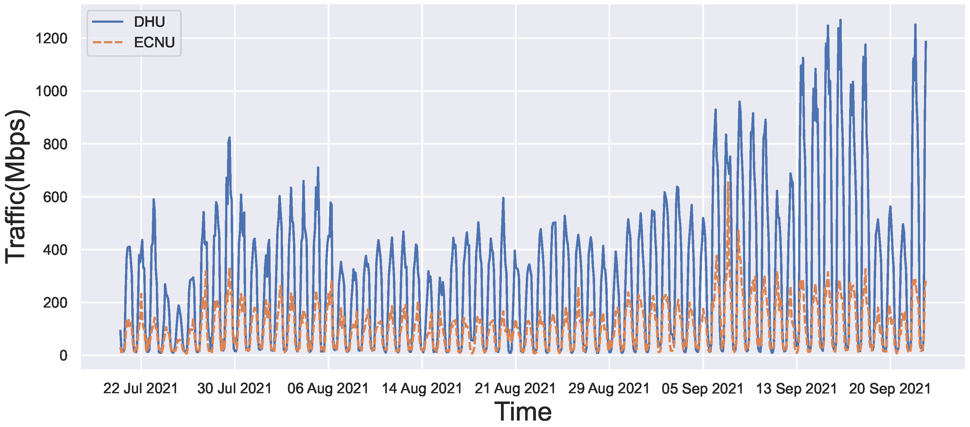
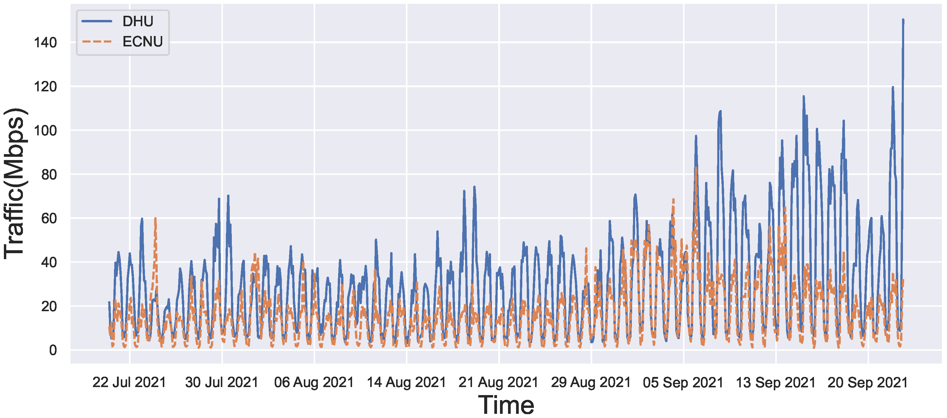
• This paper starts with analyzing the IPv6 traffic characteristics of two universities in Shanghai, i.e., Donghua University (DHU) and East China Normal University (ECNU). For each of these two universities, we show the weekday and weekend usage patterns and self-similarity of the IPv6 traffic and evaluate the correlation between IPv4 traffic and IPv6 traffic.
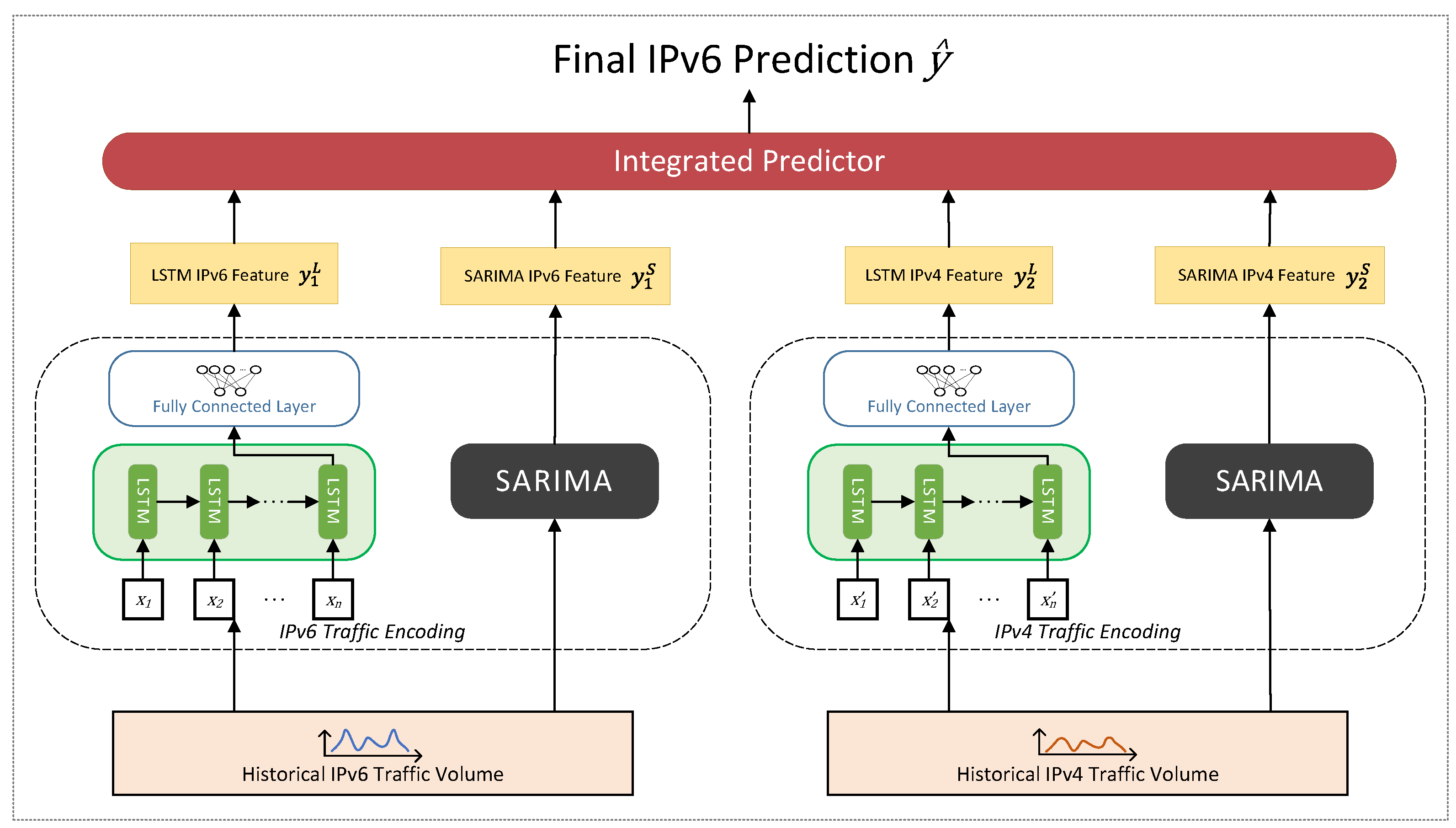
• In addition, we further dig into the problem of IPv6 traffic prediction. A new model named LSTM with seasonal ARIMA for IPv6 (LS6) is proposed to predict IPv6 network traffic with high accuracy. Considering the correlation between IPv6 and IPv4 network traffic, LS6 uses both IPv4 and IPv6 historical traffic data as the model input and leverages both the advantages of statistical and deep learning methods.
• To validate the effectiveness of our LS6 model, we conduct a series of experiments on two real-world traffic datasets. We can see that LS6 performs better than several baselines, including support vector machine (SVM), LSTM, Bi-LSTM, and phased LSTM (PLSTM).

The rest of the paper is organized as follows. Section 2 presents a review of the analysis and prediction of network traffic. In Section 3, we introduce the dataset and traffic usage feature. In Section 4, we present the detail of the proposed IPv6 traffic prediction model. In Section 5, we conduct the prediction experiment and analyze the result. We discuss several problems in Section 6. Section 7 is the conclusion.

2. Related Work

2.1. Analysis of Network Traffic

Network traffic analysis is based on different network performance indicators, such as traffic volume, latency, and packet loss rate [18]. Lutu et al. [19] found that the UK government’s lockdown policy amid the COVID-19 pandemic had dramatically changed people’s mobility patterns and Internet usage. Based on the data of UK mobile operators, the changes in user mobility and their impact on the mobile network were analyzed in detail. The overall user mobility declined by 50%, with deviations varying by region. While traffic characteristics change, operators maintained stable service as radio load decreased and per-user throughput was probably application-limited. Wang et al. [20] examined the WAN traffic characteristics in Baidu’s data centers network (DCN). They found that a significant percentage of traffic left the cluster flowing from the DC to the WAN. They further observed that traffic communications among DCs were imbalanced, i.e., a large amount of traffic was generated by a small number of DC pairs. Meanwhile, the traffic among DC services had stability over time and the stability made it possible to predict overall traffic demand.

Many prior works have analyzed the characteristics of IPv6 network traffic. Li et al. [9] studied the traffic characteristics and user behavior of the IPv4 and IPv6 networks of Xi’an Jiaotong University. They analyzed the average packet size, flow size, flow duration, and self-similarity of IPv4 and IPv6 traffic and found a significant difference between IPv4 and IPv6 traffic. Sarrar et al. [21] compared the changes in IPv6 network activities before, during, and after World IPv6 Day (8 June 2011). They found that native IPv6 traffic increased significantly while tunneled traffic did not change much during that time. Li et al. [22] analyzed IPv6 traffic based on a large-scale IPv6-based campus network with one-week traffic data. They investigated the development of IPv6 networks and studied the composition of aggregate traffic. Han et al. [10] utilized the traffic data collected on the backbone network of the China Science and Technology Network (CSTNET) and found that IPv6 traffic had been increasing rapidly from 2011 to 2013. Strowes et al. [11] conducted a statistical analysis of the IPv6 data in Yahoo and obtained the daily and weekly recurring patterns.

However, IPv6 networks are developing rapidly, and past analysis findings might not be suitable for today’s IPv6 networks. Our research analyzes the latest IPv6 traffic over campus networks to reveal the current IPv6 traffic development and leverages various analytical approaches from past work to provide a more comprehensive analysis of IPv6 traffic. In addition, we use two campus networks’ data over two months for analysis, which makes our analysis results more conclusive than many previous works.

2.2. Prediction of Network Traffic

The time series forecasting problem has always been of great importance, with influential applications in various fields such as finance [23], weather [24], transportation [25], and networking [26]. Before the era of big data, people mainly used linear models to solve time series forecasting problems, such as autoregressive (AR) [27], exponential smoothing [28], or structural time series models [29]. However, these traditional methods are only applicable when data have an explainable structure [30]. With the increasing amount of data and the improvement of computing capability, machine learning [31,32,33] has become one of the most critical methods for time series forecasting. In addition to traditional machine learning, such as SVM [34,35], the contribution of deep learning in time series forecasting is becoming more and more valuable. For multivariate time series, researchers use Convolutional Neural Networks (CNNs) [36] to extract features for prediction. Recurrent Neural Networks (RNNs) [37] can learn sequence contexts and are very helpful for time series forecasting problems. However, the flexibility of machine learning might lead to overfitting, which makes traditional linear methods more dominant when the amount of data is small [38]. One research trend is to use mixed models for time series forecasting. Hybrid models combine the advantages of traditional linear models and machine learning models to achieve better results [39,40,41].

In the past, researchers predicted future traffic with statistical methods and indicators to get regression equations. Most recent studies attempted to replace statistical methods with emerging deep learning methods to predict network traffic. Jiang [15] provided a comprehensive evaluation of deep learning methods for network traffic prediction and demonstrated that deep learning methods outperform statistical methods based on an Internet bandwidth usage dataset. Jaffry et al. [16] used LSTM to predict cellular network traffic and indicated the superior performance of LSTM over ARIMA. Katris et al. [17] proposed a hybrid forecasting method that combines neural networks with fractionally integrated ARIMA and generalized autoregressive conditional heteroskedasticity (GARCH).

Although previous studies have made efforts on network traffic prediction, to the best of our knowledge, there is still a lack of an approach to predict IPv6 traffic accurately. In particular, we are the first to utilize the correlation between IPv6 traffic and IPv4 traffic to propose a novel IPv6 traffic prediction model called LS6, which combines the advantages of the statistical method and deep learning method and makes use of the information from both IPv4 and IPv6.

3. Dataset and Traffic Usage Features

The traffic data used in this paper, including the IPv4 and IPv6 traffic volume data of the campus networks of DHU and ECNU, is collected by CERNET. The time range is from 00:00 CST on 21 July 2021 to 12:00 CST on 23 September 2021. The average traffic volume was recorded once every two hours. The IPv6 downstream and upstream network traffic is shown in Figure 1 and Figure 2, recorded with the unit of bits per second (bps). There are daily and weekly traits, with higher traffic volume during the day than at night and higher traffic volume on weekdays than on weekends.

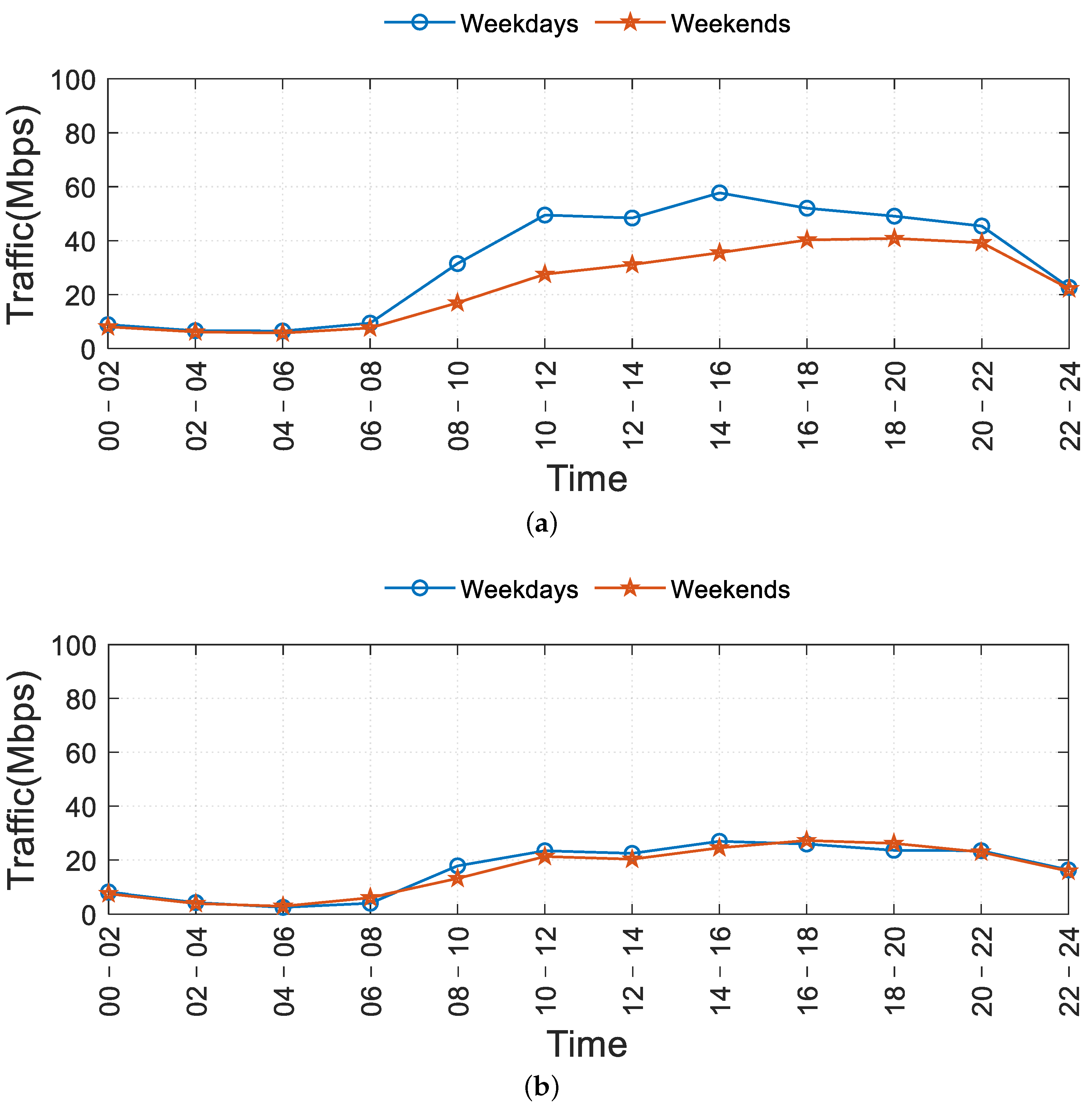
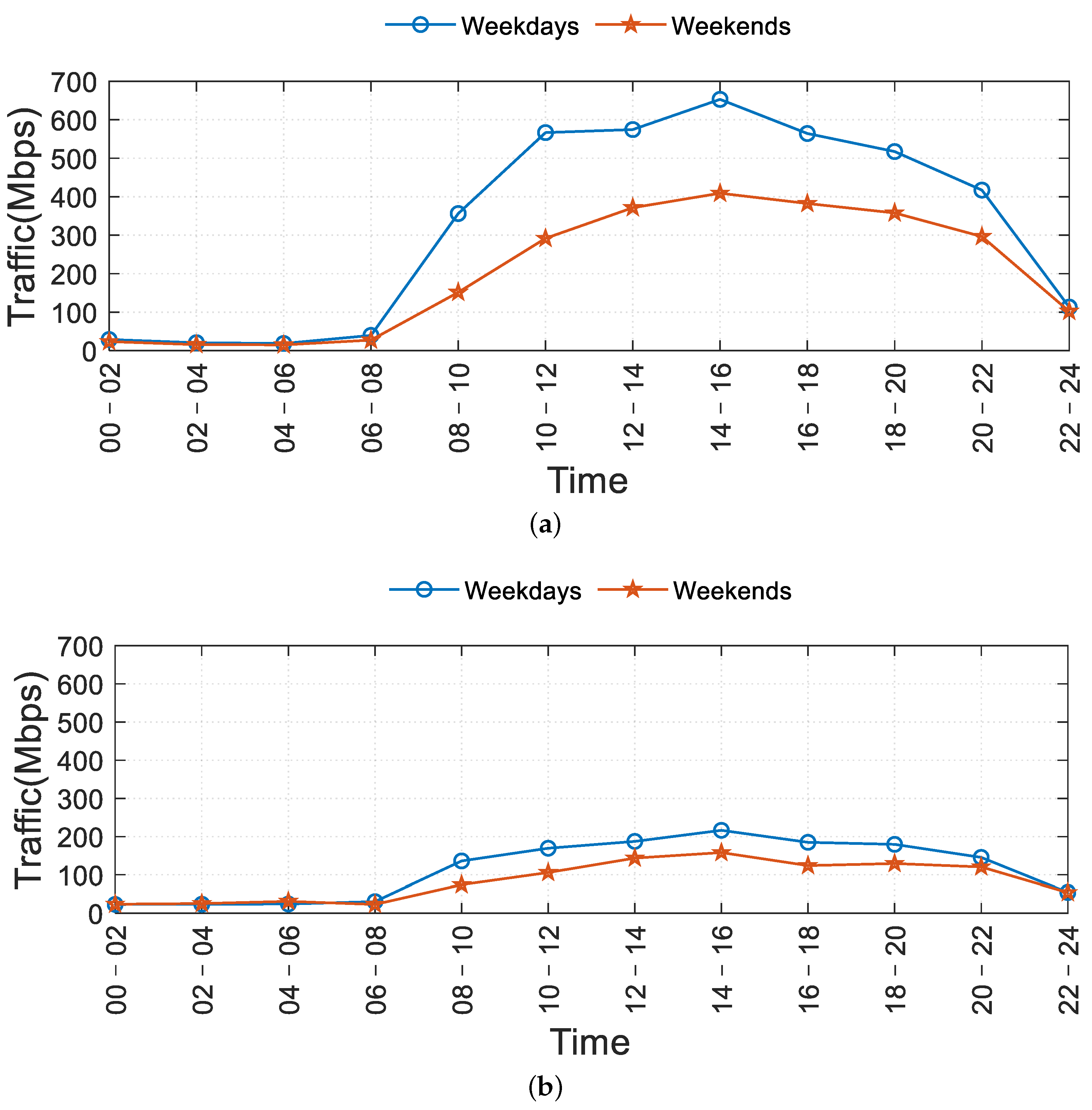
3.1. Traffic Patterns of Weekdays and Weekends

There are apparent differences in average downstream traffic volume between weekdays and weekends. The average IPv6 traffic volume of DHU on weekdays is 320.5 Mbps, while the average traffic volume on weekends is 203.7 Mbps. The average weekday IPv6 traffic volume of ECNU is 114.0 Mbps, while the average traffic volume during weekends is 84.5 Mbps. In both universities, the IPv6 network traffic usage on weekdays is higher than that on weekends. IPv6 downstream traffic patterns of weekdays and weekends are shown in Figure 3. For DHU, the IPv6 network traffic volume on weekdays ranges from 18.7 Mbps (average) from 04:00 to 06:00 CST to 653.0 Mbps (average) from 14:00 to 16:00 CST. The pattern is similar on weekends but lower, with a minimum of 15.0 Mbps and a maximum of 409.0 Mbps. In ECNU, the IPv6 network traffic volume on weekdays ranges from 23.1 Mbps (average) from 00:00 to 02:00 CST to 216.4 Mbps (average) from 14:00 to 16:00 CST. On weekends, the pattern is different as the IPv6 network traffic volume ranges from 23.1 Mbps (average) from 06:00 to 08:00 CST to 158.0 Mbps (average) from 14:00 to 16:00 CST.

The proportion of IPv6 downstream network traffic volume to total downstream network traffic volume also differs between weekdays and weekends. For DHU, the percentage of IPv6 network traffic volume on weekdays ranges from an average of 43.3% from 04:00 to 06:00 CST to 64.8% from 20:00 to 22:00 CST. On weekends, the pattern is different as the percentage of IPv6 network traffic volume ranges from an average of 39.3% from 06:00 to 08:00 CST to 63.5% from 14:00 to 16:00 CST. In ECNU, the percentage of IPv6 network traffic volume on weekdays ranges from an average of 5.3% from 00:00 to 02:00 CST to 8.6% from 04:00 to 06:00 CST. The pattern is similar on weekends but with a lower minimum of 5.2% and a higher maximum of 11.0%.

For the upstream network traffic, the average IPv6 traffic volume of DHU on weekdays is 32.2 Mbps, while the average traffic volume on weekends is 23.4 Mbps. The average weekday IPv6 traffic volume of ECNU is 16.5 Mbps, while the average traffic volume during weekends is 16.0 Mbps. In both universities, the IPv6 upstream network traffic usage on weekdays is higher than that on weekends. IPv6 upstream traffic patterns of weekdays and weekends are shown in Figure 4. For DHU, the IPv6 network traffic volume on weekdays ranges from an average of 6.5 Mbps from 04:00 to 06:00 CST to 57.7 Mbps from 14:00 to 16:00 CST. On weekends, the pattern is different as the IPv6 network traffic volume ranges from an average of 5.8 Mbps from 04:00 to 06:00 CST to 40.8 Mbps from 18:00 to 20:00 CST. In ECNU, the IPv6 network traffic volume on weekdays ranges from an average of 2.6 Mbps from 04:00 to 06:00 CST to 27.0 Mbps from 14:00 to 16:00 CST. On weekends, the pattern is different as the IPv6 network traffic volume ranges from an average of 3.0 Mbps from 04:00 to 06:00 CST to 27.3 Mbps from 16:00 to 18:00 CST.

The proportion of IPv6 upstream network traffic volume to total upstream network traffic volume also differs between weekdays and weekends. For DHU, the percentage of IPv6 network traffic volume on weekdays ranges from an average of 18.5% from 00:00 to 02:00 CST to 29.8% Mbps from 14:00 to 16:00 CST. On weekends, the pattern is different as the percentage of IPv6 network traffic volume ranges from an average of 15.9% from 00:00 to 02:00 CST to 28.0% from 18:00 to 20:00 CST. In ECNU, the percentage of IPv6 network traffic volume on weekdays ranges from an average of 2.2% from 04:00 to 06:00 CST to 3.7% from 14:00 to 16:00 CST. On weekends, the pattern is different as the proportion of IPv6 network traffic volume ranges from an average of 2.4% from 04:00 to 06:00 CST to 4.8% from 18:00 to 20:00 CST.

The network traffic pattern on weekdays is not much different from that on weekends, but the usage volume is smaller on weekends. Therefore, the IPv6 users from these two universities are more active during weekdays, which is the opposite of what happens in commercial networks [11]. In addition, we find that the percentage of IPv6 network traffic volume in DHU decreases slightly over the weekends, while the percentage of IPv6 network traffic volume in ECNU increases slightly over the weekends.

3.2. Self-Similarity Analysis

Since studies found that the self-similarity model can describe network traffic’s characteristics more accurately than the traditional Poisson traffic model, it has been widely used in Internet-related studies [9,42,43]. The Hurst exponent (H) is a classic metric used to describe the self-similarity characteristic of the network traffic. To calculate the R/S statistic from a stationary process, it approximately satisfies

$$E[R\left(n\right)/S\left(n\right)]=C{n}^H,n\to \infty$$

(1)

where H is the Hurst exponent varying between 0 and 1, n is the number of data slots in a stationary process, $R\left(n\right)$ is the range of the cumulative deviations from the mean in the first n data slots, $S\left(n\right)$ is the standard deviation of the first n data slots, $E\left(x\right)$ is the expected value, and C is a constant. Clearly, $H>0.5$ is a necessary condition for the existence of self-similarity, and a time series with larger H has stronger self-similarity. A value of $H=0.5$ indicates that the series is completely uncorrelated and can be described as a random walk, whereas $H<0.5$ suggests that the series tends to switch between high and low values in the long term.

We estimate the value of the Hurst exponent [44] using the aggregate variance method (A/V), the R/S method, and the periodogram method (P) and compare the Hurst exponents of IPv6 and IPv4 traffic volume.

• The aggregate variance method plots the sample variance versus the block size of each aggregation level on a log-log plot. If the series is self-similar, the plot will be a line with slope $\beta$ greater than -1. The H is estimated by $H=1+\beta /2$.
• $R/S$ method uses the rescaled range statistic ($R/S$ statistic). The $R/S$ statistic is the range of the cumulative deviations of a time series sequence from its mean, divided by its standard deviation. The method plots the R/S statistic versus the number of points of the aggregated series and the plot should be linear with a slope. The estimation of the Hurst exponent is the slope.
• Periodogram method plots the the spectral density of a time series versus the frequencies on a log-log plot. The slope of the plot is the estimate of H.

The results are summarized in

Table 1. The values of Hurst exponents of IPv4 and IPv6 traffic.

Traffic Category	Method	IPv4 Downstream	IPv6 Downstream	IPv4 Upstream	IPv6 Upstream
	R/S	0.6703	0.6609	0.6962	0.6957
DHU	A/V	0.6936	0.6671	0.6355	0.6984
	P	0.5936	0.6315	0.5503	0.6285
	R/S	0.7159	0.6990	0.8104	0.8090
ECNU	A/V	0.6652	0.6698	0.8253	0.7843
	P	0.5476	0.6740	0.6771	0.7349

. As it shows, in both universities, the IPv4 Hurst exponents of the upstream or downstream traffic are similar to the IPv6 Hurst exponents, while in a study on a campus network in 2012 [9], there was a big gap between the self-similarity of IPv4 traffic and that of IPv6 traffic. The results imply the difference between IPv6 and IPv4 traffic is much smaller than earlier results in [9].

3.3. Correlation Analysis

In this subsection, we use Pearson [45], Spearman [46], and Kendall [47] correlation coefficients to measure the correlation between IPv4 traffic and IPv6 traffic. All of them are widely used in correlation analysis [48,49,50].

The Pearson correlation coefficient between the two time series X and Y is defined as

$${\rho }_{X,Y}=\frac{E\left[(X-{\mu }_X)(Y-{\mu }_Y)\right]}{{\sigma }_X{\sigma }_Y}$$

(2)

where ${\rho }_{X,Y}$ is the Pearson correlation coefficient varying between −1 and 1, ${\mu }_X$ and ${\mu }_Y$ are the means of X and Y, and ${\sigma }_X$ and ${\sigma }_Y$ are the standard deviations of X and Y.

The Spearman rank correlation coefficient between two time series $X=\{x_1,x_2,\dots ,x_n\}$ and $Y=\{y_1,y_2,\dots ,y_n\}$ could be calculated as

$${\rho }_{X,Y}=1-\frac{6\sum d_i^2}{n(n^2-1)}$$

(3)

where ${\rho }_{X,Y}$ is the Spearman rank correlation coefficient varying between −1 and 1, $d_i$ is the difference between the ranks of corresponding values of $x_i$ and $y_i$, and n is the length of time series.

The Kendall rank correlation coefficient between two time series $X=\{x_1,x_2,\dots ,x_n\}$ and $Y=\{y_1,y_2,\dots ,y_n\}$ is

$${\rho }_{X,Y}=\frac{\frac{1}{2}n(n-1)-d}{\frac{1}{2}n(n-1)}$$

(4)

where ${\rho }_{X,Y}$ is the Kendall rank correlation coefficient varying between -1 and 1, and d is the number of discordant pairs in all $\{x_i,y_j\}$, n is the length of time series.

A value of ${\rho }_{X,Y}=0$ indicates that the two series are completely uncorrelated. The closer the correlation coefficient is to 1(−1), the stronger the positive (negative) correlation is. As shown in

Table 2. The correlation coefficient between IPv4 and IPv6 traffic.

Traffic Category	Method	Downstream	Upstream
	Pearson	0.934	0.842
DHU	Spearman	0.948	0.887
	Kendall	0.804	0.699
	Pearson	0.907	0.779
ECNU	Spearman	0.915	0.844
	Kendall	0.740	0.660

, the smallest correlation coefficients between IPv4 downstream traffic and IPv6 downstream traffic are 0.804 and 0.740 for DHU and ECNU, respectively. The smallest correlation coefficients between IPv4 upstream traffic and IPv6 upstream traffic are 0.699 and 0.660 for DHU and ECNU, respectively. Therefore, there is a strong positive correlation between the IPv4 traffic and IPv6 traffic in both universities. Additionally, we can see that the correlation between downstream traffic is stronger than that between upstream traffic.

4. IPv6 Traffic Prediction Model

4.1. Problem Formulation

After analyzing the characteristics of the IPv6 traffic of DHU and ECNU, we move further into the following challenge—whether we are able to predict the traffic volume of the next time slot based on the historical data. Specifically, we consider a one-step prediction problem of IPv6 traffic feeding 2-hour fine-grained IPv4 and IPv6 traffic time series of length n to model and predict the IPv6 traffic volume of the next time slot. The IPv6 traffic volume to be predicted is defined as y. The input is two time series, denoted as $V=\{x_1,x_2,\dots ,x_n\}$ and $V^{{}^{\prime }}=\{x_1^{{}^{\prime }},x_2^{{}^{\prime }},\dots ,x_n^{{}^{\prime }}\}$, where n is the time step, $x_i$ is the IPv6 traffic volume and $x_i^{{}^{\prime }}$ is the IPv4 traffic volume.

4.2. The LS6 Model

This subsection introduces the detail of the proposed LS6 model. We first give the overview of the proposed model LS6 and then introduce the components of LS6.

4.2.1. Model Overview

As shown in Figure 5, there are two key components of our approach. First, we use a traffic encoding component to take historical traffic data as input and automatically extract two types of features with deep learning and statistical methods. Second, we introduce an integrated predictor component, focusing on combining the outputs of deep learning and statistical methods to get the final prediction. In the traffic encoding component, we leverage two independent seasonal ARIMA (SARIMA) modules and two independent LSTM networks to predict IPv6 and IPv4 network traffic volume in the next time slot with previous traffic volume. To capture the relationship between IPv6 and IPv4 traffic and combine the advantages of LSTM and SARIMA, we feed $y_1^L$,$y_1^S$,$y_2^L$, and $y_2^S$, the extracted features of IPv6 and IPv4 traffic from LSTM and SARIMA to a multilayer perceptron (MLP) model in the integrated predictor module and get the final prediction $\widehat{y}$. In the following subsections, we introduce the two modules in detail.

4.2.2. Traffic Encoding

The traffic encoding component is responsible for extracting traffic features with deep learning and statistical methods. RNNs such as LSTM can extract features automatically, while SARIMA provides a better theoretical interpretation for time series prediction problems [15]. Thus, we consider both LSTM and SARIMA as extractors of network traffic features in the traffic encoding module.

As traffic prediction is a time series prediction problem, an RNN, which can extract the sequential feature, is often used to solve such problems. We pick LSTM, a representative RNN, as the deep learning method to predict traffic volume and regard the prediction as a feature. LSTM is a variant of RNN for vanishing gradient problems, which has been widely used in time series prediction [23,25,51]. Figure 6a shows that each LSTM cell consists of three gates—the forget gate, the input gate, and the output gate. The cell state $C_t$ and hidden state $h_t$ for the current cell are generated by $C_{t-1}$ and $h_{t-1}$ from the last cell and input $x_t$ passing through the three gates. The forget gate selectively bars the state value from the previous time step $C_{t-1}$. The input gate decides which information is added to $C_t$. The output gate integrates the information from the forget gate and the input gate to get the output $h_t$. As shown in Figure 6b, one layer of the LSTM network is formed by chained LSTM cells. Each cell receives the previous cell state and hidden state and then generates a new cell state and hidden state for the next cell. The number of data observations used for prediction is disclosed by the number of cells in an LSTM network. The mathematical expressions of LSTM are shown as follows:

$$f_t=\sigma (W_f{x}_t+U_f{h}_{t-1}+b_f)$$

(5)

$$i_t=\sigma (W_i{x}_t+U_i{h}_{t-1}+b_i)$$

(6)

$$o_t=\sigma (W_o{x}_t+U_o{h}_{t-1}+b_o)$$

(7)

where $x_t$ is the current input and $h_{t-1}$ is the previous hidden state. $f_t$, $i_t$, and $o_t$ are the output of the forget, input, and output gates, respectively. $\{W_f,U_f,b_f\}$, $\{W_i,U_i,b_i\}$, and $\{W_o,U_o,b_o\}$ are the parameters of the forget, input and output gates, respectively.

$${\tilde{C}}_t=tanh(W_c{x}_t+U_c{h}_{t-1}+b_c)$$

(8)

$$C_t=f_t\ast C_{t-1}+i_t\ast \tilde{C}$$

(9)

$$h_t=o_t\ast tanh\left(C_t\right)$$

(10)

where ${\tilde{C}}_t$ is the candidate memory, $C_t$ and $h_t$ are the current cell memory and hidden state, and $\{W_c,U_c,b_c\}$ are the parameters of the candidate memory network.

In our case, input $x_t$ is the network traffic volume while the number of observations is the number of selected time steps, n. The output of LSTM is the hidden state of the final cell ($h_n$) and is fed to a fully connected layer to get the prediction.

We then leverage SARIMA [13] for traffic prediction. SARIMA (or seasonal ARIMA) is an extension of ARIMA, which can better forecast time series with periodicity. The SARIMA model can be defined by $SARIMA(p,d,q){(P,D,Q)}_s$, where p is the order of the non-seasonal autoregressive model, q is the order of non-seasonal moving average model, P is the order of seasonal autoregressive model, Q is the order of seasonal moving average model, d is the number of non-seasonal differences, D is the number of seasonal differences, and s is the periodic term. We feed both past IPv4 and IPv6 traffic data into SARIMA and LSTM, respectively, to acquire prediction results of the future traffic volume, which are regarded as traffic features of the next time slot.

4.2.3. Integrated Predictor

The integrated predictor combines the advantages of LSTM and SARIMA to build an integrated model which incorporates the deep learning approach with statistical prediction algorithm. The integrated predictor is an MLP model, which is a fully-connected class of feedforward neural networks. The MLP model consists of one input layer, one output layer, and one hidden layer using nonlinear activation, for example, the ReLU function. The input layer accepts the input information and then transforms it into a hidden layer. The output layer performs the prediction task with the output of the hidden layer. Due to the correlation between IPv4 and IPv6 traffic shown in Section 3.3, we consider the prediction of IPv6 traffic by LSTM and SARIMA using both IPv4 and IPv6 traffic data. In order to strengthen the weight of IPv4 traffic in predicting IPv6 traffic, we convert the predicted value of IPv4 traffic into the proportion of IPv6 traffic in the total traffic. The process is as follows:

$$y_{prop}^S=\frac{\alpha y_1^S}{y_1^S+y_2^S}$$

(11)

$$y_{prop}^L=\frac{\alpha y_1^L}{y_1^L+y_2^L}$$

(12)

where $y_{prop}^S$ is the proportion of IPv6 traffic in the total traffic with SARIMA results, $y_{prop}^L$ is the proportion of IPv6 traffic in the total traffic with LSTM results, $y_1^L$ and $y_2^L$ are the IPv6 and IPv4 traffic predictions by LSTM, $y_1^S$ and $y_2^S$ are the IPv6 and IPv4 traffic predictions by SARIMA, and $\alpha$ is a hyperparameter between 0 and 1, which limits the effect of proportion on the model.

$y_{prop}^S$, $y_{prop}^L$, $y_1^L$, and $y_1^S$ are fed to the MLP model to learn the weights of features. The output of the MLP model is the final predicted volume of the IPv6 traffic $\widehat{y}$.

4.3. Learning and Prediction

To learn the parameters of LS6, we adopt mean squared error (MSE) as the loss function to train the model, which is formulated as:

$$\mathcal{L}=\frac{1}{N}\sum _{i=1}^N{({\widehat{y}}_i-y_i)}^2$$

(13)

where N is the number of training samples.

4.4. Summary

The proposed model LS6 combines the advantages of the deep learning model LSTM and statistical model SARIMA to predict the future IPv6 traffic volume with the information on historical IPv6 and IPv4 traffic volume. We consider LSTM and SARIMA as feature extractors and pre-train them. We feed IPv6 and IPv4 historical traffic volume information into LSTM and SARIMA, respectively, and get four intermediate values. The four intermediate values are then input into an MLP, and the contribution of each value to the final predicted value is trained. The output of the MLP is the final predicted value. We believe that the superiority of LS6 lies in exploiting the correlation between IPv4 and IPv6 and combining the advantages of deep learning and statistical methods.

5. Evaluation

5.1. Datasets

We use the real-world downstream traffic volume data in two campus networks of DHU and ECNU. The time range is from 00:00 CST on 21 July 2021 to 12:00 CST on 23 September 2021. The average traffic volume was recorded once every two hours. In chronological order, we select the traffic data within the first 70% of the time range as training data, the following 20% as validation data, and the last 10% as test data to evaluate the performance.

5.2. Experimental Setup

(1) Implementation details: We pre-train the two LSTM and two SARIMA models by predicting the IPv4 traffic volume or IPv6 traffic volume of the next time slot. We train a dedicated LS6 model for each dataset. We implement the deep learning model using PyTorch and build the SARIMA model by Python’s statsmodels library. The experiments are implemented on a server with an Intel i7-9750H CPU, an NVIDIA GeForce RTX 1650 8GB graphics card, and a DDR4 8GB memory. The LSTM model has a hidden layer with 10-dimension hidden units, containing 12 LSTM cells, so the input historical time slot number is fixed as 12. For SARIMA, we set the seasonal cycle as 12 and select the best SARIMA model based on the Akaike information criterion (AIC) [52]. The MLP is composed of one input and one output layer, and one hidden layer with 100 units using the ReLU activation function. We select Adam [53] as the optimizer for the deep learning model. The learning rate is set to 0.001 and the batch size is set to 8 in DHU and 16 in ECNU. The hyperparameter $\alpha$ is set to 0.01.

(2) Baselines: To verify the prediction performance of our model, we compare LS6 with some existing approaches.

• Naive-2h: Naive-2h uses the IPv6 traffic volume of the previous time slot as the predicted value. We use Naive-2h to show the traffic difference between adjacent time slots.
• Naive-24h: Naive-24h uses the IPv6 traffic volume 24 h ago, in other words, the traffic value of the corresponding time slot of the previous day, as the predicted value. We use Naive-24h to show the traffic difference between adjacent days.
• ARIMA: We only use the previous IPv6 traffic data to fit an ARIMA model and then predict the IPv6 traffic volume at the next time slot with ARIMA.
• SARIMA: We only use the previous IPv6 traffic data to fit a SARIMA model which is used as a part of traffic encoding in LS6 and then predict IPv6 traffic volume at the next time slot with SARIMA.
• SVM: SVM is a classic supervised machine learning algorithm which can be used for regression. We only use the IPv6 traffic data to train an SVM and use the output of the SVM as the predicted IPv6 traffic volume.
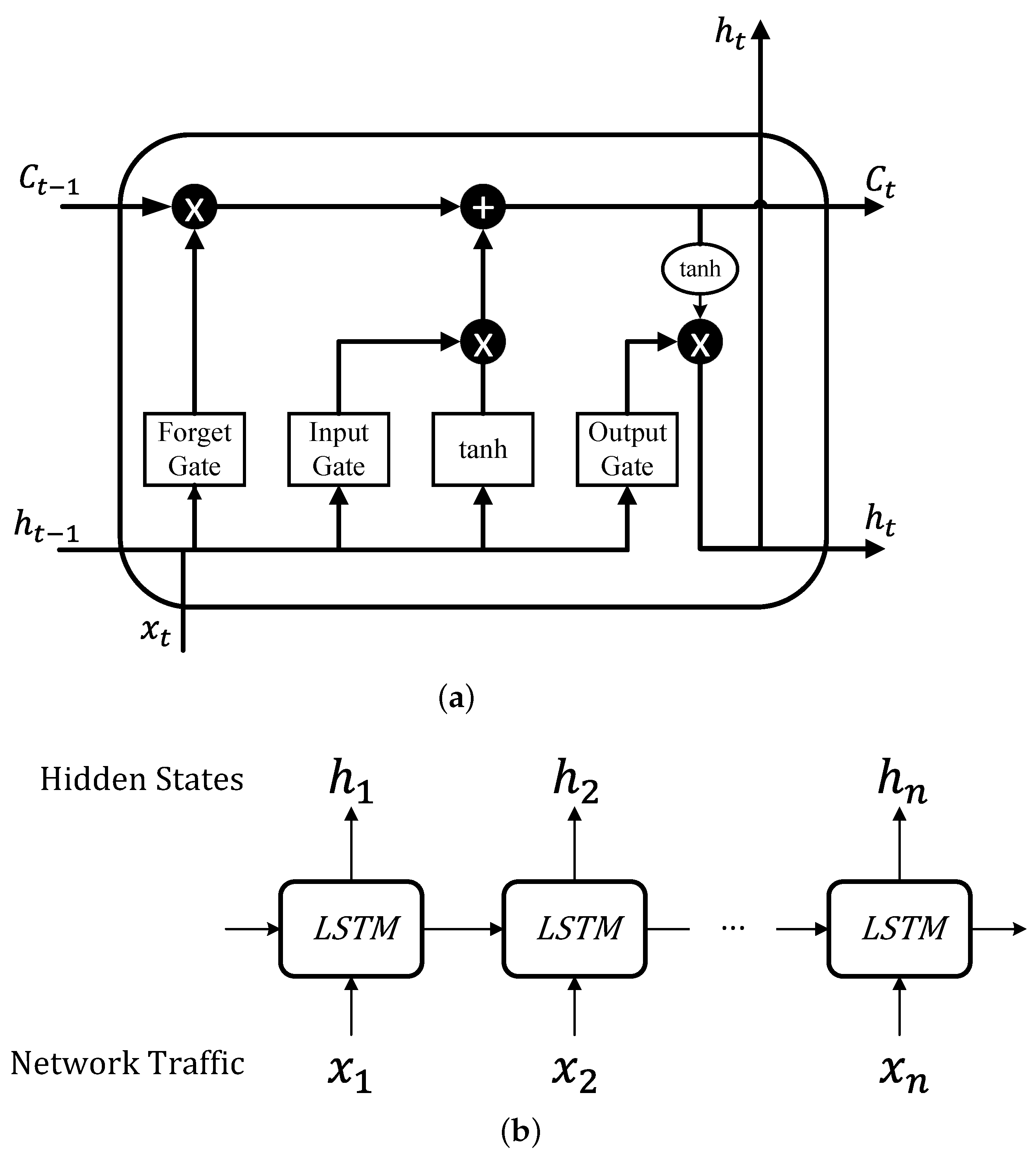
• LSTM: We only use the IPv6 traffic data to train an LSTM network which is used as a part of traffic encoding in LS6. The output of the LSTM network is fed to a fully connected layer to get the predicted IPv6 traffic volume.
• Bi-LSTM [54]: Bidirectional LSTM is a variant of LSTM composed of a forward LSTM and a backward LSTM, which can save information from both the past and future. We train it the same way we train the LSTM network. The output of the Bi-LSTM network is fed to a fully connected layer to get the predicted IPv6 traffic volume.
• PLSTM [55]: Phased LSTM (PLSTM) is a variant of LSTM and extends the LSTM model by adding a new time gate, which achieves faster convergence than the vanilla LSTM on long sequences tasks. It has also been applied in time series prediction [56,57,58,59]. We train it the same way we train the LSTM network. The output of the PLSTM network is fed to a fully connected layer to get the predicted IPv6 traffic volume.

(3) Metrics: The evaluation metric mean absolute percentage error (MAPE) compares the prediction performance of different approaches. MAPE has been widely used for time series prediction problems in a variety of domains such as network traffic [60], vehicle speed [61], electrical power [62], and remaining service duration of bearings [63]. Denoting the real traffic volume as y and the predicted traffic volume as $\widehat{y}$, the MAPE metric is defined as follows:

$$MAPE=\frac{100\%}{N}\sum _1^N\left|\frac{{\widehat{y}}_i-y_i}{y_i}\right|$$

(14)

where N is the number of data samples in the test set. The smaller the MAPE value is, the better the prediction performance is.

5.3. Result and Analysis

The results of MAPE are listed in

Table 3. Prediction performance of LS6 and baseline methods on different datasets.

Dataset	Model	MAPE
	Naive-2h	0.7664
	Naive-24h	0.2878
	ARIMA	0.7556
	SARIMA	0.2675
DHU	SVM	0.7471
	LSTM	0.4557
	Bi-LSTM	0.3678
	PLSTM	0.7975
	LS6	0.2410
	Naive-2h	0.6062
	Naive-24h	0.3546
	ARIMA	0.7418
	SARIMA	0.3175
ECNU	SVM	0.6998
	LSTM	0.3367
	Bi-LSTM	0.5479
	PLSTM	0.4509
	LS6	0.3146

. As for the baselines, SARIMA achieves the best performance. Nevertheless, LS6 performs the best, while SARIMA ranks second among all approaches. For both datasets, the results clearly corroborate the superiority of the proposed LS6 in IPv6 traffic prediction. Specifically, the MAPE value of LS6 in DHU is 2.65% lower than that of SARIMA, and this number is 0.29% lower in ECNU.

5.4. Ablation Study

To study how different components of LS6 contribute to the prediction, we conduct an ablation study. Seven variants of LS6 are considered: (1) LS6 (w/o SARIMA_v6): the model without the SARIMA for extracting the IPv6 traffic feature; (2) LS6 (w/o SARIMA_v4): the model without the SARIMA for extracting the IPv4 traffic feature; (3) LS6 (w/o LSTM_v6): the model without the LSTM for extracting the IPv6 traffic feature; (4) LS6 (w/o LSTM_v4): the model without the LSTM for extracting the IPv4 traffic feature; (5) LS6 (w/o IPv4): the model without the IPv4 traffic input; (6) LS6 (w/o SARIMA): the model without SARIMA; (7) LS6 (w/o LSTM): the model without LSTM.

As shown in

Table 4. Prediction performance of LS6 and variants (ECNU).

Model	MAPE
LS6 (w/o SARIMA_v6)	0.4882
LS6 (w/o SARIMA_v4)	0.4108
LS6 (w/o LSTM_v6)	1.2277
LS6 (w/o LSTM_v4)	0.4045
LS6 (w/o IPv4)	0.3569
LS6 (w/o SARIMA)	0.3776
LS6 (w/o LSTM)	0.7950
LS6	0.3146

, all components are important for LS6. Specifically, the LSTM for extracting the IPv6 traffic feature is the most critical part. We also find that the importance of IPv4 traffic and SARIMA is proven.

6. Discussion

6.1. Training Using Both Datasets

In Section 5, we train a dedicated model for each dataset. In this subsection, we try to discuss the prospective improvement of training LS6 using both datasets. We combine the training data of two datasets to increase the number of training samples. We use the combined training data to train a new LS6 model. Finally, we evaluate the performance of LS6 using the test data of each of the two datasets. As shown in

Table 5. Prediction performance of LS6 trained with a single training data and combined training data.

Dataset	Model	MAPE
DHU	LS6	0.2410
	LS6 (combine)	0.2317
ECNU	LS6	0.3146
	LS6 (combine)	0.2953

, we find that the LS6 trained with the combined training data performs better in both datasets. It indicates that the ISPs could use data from different networks to train LS6 to achieve better results.

6.2. The Influence of the 24 h Period

From Figure 2, we can find there exists a 24 h period in the IPv6 traffic change, which is verified by the good performance of Naive-24h. Therefore, the 24 h traffic difference, which means the difference between the traffic volume and the traffic volume 24 h ago could be an alternative prediction choice for improving the model performance.

In this subsection, we predict the 24 h traffic differences rather than the exact volume of future traffic to study the influence of the 24 h period. We take the predicted 24 h traffic difference plus the traffic volume 24 h ago as the predicted traffic volume, and then calculate the model performance in the MAPE metric. As shown in

Table 6. Prediction performance of LS6 and baseline methods in different training approaches.

Dataset	Model	MAPE (24 h)	MAPE (Directly)
	SVM	0.6432	0.7471
	LSTM	0.4143	0.4557
DHU	Bi-LSTM	0.4529	0.3678
	PLSTM	0.3215	0.7975
	LS6	0.3998	0.2410
	SVM	0.3992	0.6998
	LSTM	0.3287	0.3367
ECNU	Bi-LSTM	0.3263	0.5479
	PLSTM	0.3453	0.4509
	LS6	0.3428	0.3146

, the MAPE (24 h) is the model performance of predicting the 24 h traffic differences while the MAPE (Directly) is the model performance of predicting the traffic volume directly. The baseline machine learning models’ performance is significantly improved by predicting the 24 h traffic differences as it can eliminate the period influence.

However, the LS6 model does not perform better while focusing on predicting the 24 h traffic differences. Still, the LS6 model predicting the exact volume of the IPv6 traffic performs best among all models in the two training approaches. We believe it is because the SARIMA in the LS6 can make good use of the period information. Eliminating the 24 h period influence might not be beneficial for our LS6 model.

6.3. Limitation

One main limitation of our work is that we only analyze and predict the IPv6 traffic based on the traffic volume data of universities in Shanghai. Therefore, our analysis results could only present the situation of universities in Shanghai, and the generalization of our proposed prediction model remains to be further validated.

7. Conclusions and Future Work

With the development of IPv6, it is increasingly crucial to study IPv6 traffic patterns. To this end, we analyzed the weekday/weekend patterns, the self-similarity of the IPv6 traffic, and the correlation between IPv6 and IPv4 traffic for two universities in Shanghai, China. The network traffic distribution on weekdays is not much different from that on weekends, while the traffic usage is smaller on weekends. It shows that the IPv6 users of the two campus networks are more active during weekdays. We evaluate the self-similarity by estimating the value of the Hurst exponent. The Hurst exponents of the IPv6 traffic are similar to those of IPv4 traffic, which implies that the difference between IPv6 and IPv4 traffic is smaller than before. As the smallest correlation coefficients between IPv4 traffic and IPv6 traffic are 0.699 and 0.660 for DHU and ECNU, respectively, there is a strong positive correlation between IPv6 traffic and IPv4 traffic in the two universities.

To better predict IPv6 traffic, we proposed a new approach called LS6 by combining the advantages of LSTM and seasonal ARIMA and utilizing the correlation between IPv6 and IPv4 traffic. Based on two real-world IPv6 traffic datasets, the experiments show that LS6 achieves a lower prediction error (MAPE) than eight baselines. For example, the MAPE value of LS6 in DHU is 2.65% lower than that of the best baseline. The results confirm that our proposed model LS6 can better predict the IPv6 traffic volume than existing methods.

Overall, our research is beneficial for ISPs to allocate and manage network resources. In our future work, we will try to obtain more IPv6 traffic volume datasets in other cities worldwide. In addition, we will further study the IPv6 traffic prediction with model combinations. We will improve the prediction performance by enhancing the LSTM model with an additional attention layer and by considering other features, such as the Hurst exponent and differences between weekdays and weekends.

References

1. Li, F.; Freeman, D. Towards A User-Level Understanding of IPv6 Behavior. In Proceedings of the 2020 ACM Internet Measurement Conference (IMC), Virtual Event, USA, 27–29 October 2020; pp. 428–442. [Google Scholar]
2. Google IPv6 Statistics. Available online: https://www.google.com/intl/en/ipv6/statistics.html (accessed on 13 February 2022).
3. Rye, E.C.; Beverly, R.; Claffy, K.C. Follow the scent: Defeating IPv6 prefix rotation privacy. In Proceedings of the 2021 ACM Internet Measurement Conference (IMC), Virtual Event, USA, 2–4 November 2021; pp. 739–752. [Google Scholar]
4. Hermann, S.; Fabian, B. A Comparison of Internet Protocol (IPv6) Security Guidelines. Future Internet 2014, 6, 1–60. [Google Scholar] [CrossRef] [Green Version]
5. Cui, Y.; Dong, J.; Wu, P.; Wu, J.; Metz, C.; Lee, Y.L.; Durand, A. Tunnel-Based IPv6 Transition. IEEE Internet Comput. 2012, 17, 62–68. [Google Scholar] [CrossRef]
6. Fang, R.; Han, G.; Wang, X.; Bao, C.; Li, X.; Chen, Y. Speeding up IPv4 connections via IPv6 infrastructure. In Proceedings of the SIGCOMM’21 Poster and Demo Sessions, Virtual Event, USA, 23–27 August 2021; pp. 76–78. [Google Scholar]
7. Joshi, M.; Hadi, T.H. A Review of Network Traffic Analysis and Prediction Techniques. arXiv 2015, arXiv:1507.05722. [Google Scholar]
8. Ramakrishnan, N.; Soni, T. Network traffic prediction using recurrent neural networks. In Proceedings of the 17th IEEE International Conference on Machine Learning and Applications (ICMLA), Orlando, FL, USA, 17–20 December 2018; pp. 187–193. [Google Scholar]
9. Li, Q.; Qin, T.; Guan, X.; Zheng, Q. Empirical analysis and comparison of IPv4-IPv6 traffic: A case study on the campus network. In Proceedings of the 18th IEEE International Conference on Networks (ICON), Singapore, 12–14 December 2012; pp. 395–399. [Google Scholar]
10. Han, C.; Li, Z.; Xie, G.; Uhlig, S.; Wu, Y.; Li, L.; Ge, J.; Liu, Y. Insights into the issue in IPv6 adoption: A view from the Chinese IPv6 Application mix. Concurr. Comput. Pract. Exp. 2016, 28, 616–630. [Google Scholar] [CrossRef] [Green Version]
11. Strowes, S.D. Diurnal and Weekly Cycles in IPv6 Traffic. In Proceedings of the 2016 Applied Networking Research Workshop (ANRW), Berlin, Germany, 16 July 2016; pp. 65–67. [Google Scholar]
12. Urushidani, S.; Fukuda, K.; Koibuchi, M.; Nakamura, M.; Abe, S.; Ji, Y.; Aoki, M.; Yamada, S. Dynamic Resource Allocation and QoS Control Capabilities of the Japanese Academic Backbone Network. Future Internet 2010, 2, 295–307. [Google Scholar] [CrossRef] [Green Version]
13. Valipour, M. Long-term runoff study using SARIMA and ARIMA models in the United States. Meteorol. Appl. 2015, 22, 592–598. [Google Scholar] [CrossRef]
14. Hochreiter, S.; Schmidhuber, J. Long Short-Term Memory. Neural Comput. 1997, 9, 1735–1780. [Google Scholar] [CrossRef]
15. Jiang, W. Internet traffic prediction with deep neural networks. Internet Technol. Lett. 2022, 5, e314. [Google Scholar] [CrossRef]
16. Jaffry, S.; Hasan, S.F. Cellular Traffic Prediction using Recurrent Neural Networks. In Proceedings of the 5th IEEE International Symposium on Telecommunication Technologies (ISTT), Shah Alam, Malaysia, 9–11 November 2020; pp. 94–98. [Google Scholar]
17. Katris, C.; Daskalaki, S. Dynamic Bandwidth Allocation for Video Traffic Using FARIMA-Based Forecasting Models. J. Netw. Syst. Manag. 2019, 27, 39–65. [Google Scholar] [CrossRef]
18. Abbasi, M.; Shahraki, A.; Taherkordi, A. Deep Learning for Network Traffic Monitoring and Analysis (NTMA): A Survey. Comput. Commun. 2021, 170, 19–41. [Google Scholar] [CrossRef]
19. Lutu, A.; Perino, D.; Bagnulo, M.; Frias-Martinez, E.; Khangosstar, J. A Characterization of the COVID-19 Pandemic Impact on a Mobile Network Operator Traffic. In Proceedings of the 2020 ACM Internet Measurement Conference (IMC), Virtual Event, USA, 27–29 October 2020; pp. 19–33. [Google Scholar]
20. Wang, Z.; Li, Z.; Liu, G.; Chen, Y.; Wu, Q.; Cheng, G. Examination of WAN traffic characteristics in a large-scale data center network. In Proceedings of the 2021 ACM Internet Measurement Conference (IMC), Virtual Event, USA, 2–4 November 2021; pp. 1–14. [Google Scholar]
21. Sarrar, N.; Maier, G.; Ager, B.; Sommer, R.; Uhlig, S. Investigating IPv6 Traffic - What Happened at the World IPv6 Day? In Proceedings of the 13th International Conference on Passive and Active Network Measurement (PAM), Vienna, Austria, 12–14 March 2012; pp. 11–20. [Google Scholar]
22. Li, F.; An, C.; Yang, J.; Wu, J.; Zhang, H. A study of traffic from the perspective of a large pure IPv6 ISP. Comput. Commun. 2014, 37, 40–52. [Google Scholar] [CrossRef]
23. Cao, J.; Li, Z.; Li, J. Financial time series forecasting model based on CEEMDAN and LSTM. Phys. Stat. Mech. Its Appl. 2019, 519, 127–139. [Google Scholar] [CrossRef]
24. Karevan, Z.; Suykens, J.A. Transductive LSTM for time-series prediction: An application to weather forecasting. Neural Netw. 2020, 125, 1–9. [Google Scholar] [CrossRef]
25. Xie, Q.; Guo, T.; Chen, Y.; Xiao, Y.; Wang, X.; Zhao, B.Y. Deep Graph Convolutional Networks for Incident-Driven Traffic Speed Prediction. In Proceedings of the 29th ACM International Conference on Information & Knowledge Management (CIKM), Virtual Event, Ireland, 19–23 October 2020; pp. 1665–1674. [Google Scholar]
26. Madan, R.; Mangipudi, P.S. Predicting computer network traffic: A time series forecasting approach using DWT, ARIMA and RNN. In Proceedings of the 2018 Eleventh International Conference on Contemporary Computing (IC3), Noida, India, 2–4 August 2018; pp. 1–5. [Google Scholar]
27. Nassar, S.; Schwarz, K.P.; El-Sheimy, N.; Noureldin, A. Modeling inertial sensor errors using autoregressive (AR) models. Navigation 2004, 51, 259–268. [Google Scholar] [CrossRef]
28. Winters, P.R. Forecasting sales by exponentially weighted moving averages. Manag. Sci. 1960, 6, 324–342. [Google Scholar] [CrossRef]
29. Harvey, A.C.; Shephard, N. 10 Structural time series models. In Econometrics; Handbook of Statistics; Elsevier: Amsterdam, The Netherlands, 1993; Volume 11, pp. 261–302. [Google Scholar]
30. Lara-Benítez, P.; Carranza-García, M.; Riquelme, J.C. An Experimental Review on Deep Learning Architectures for Time Series Forecasting. Int. J. Neural Syst. 2021, 31, 2130001. [Google Scholar] [CrossRef]
31. Abdellah, A.R.; Mahmood, O.A.; Kirichek, R.; Paramonov, A.; Koucheryavy, A. Machine Learning Algorithm for Delay Prediction in IoT and Tactile Internet. Future Internet 2021, 13, 304. [Google Scholar] [CrossRef]
32. Alzahrani, A.O.; Alenazi, M.J. Designing a Network Intrusion Detection System Based on Machine Learning for Software Defined Networks. Future Internet 2021, 13, 111. [Google Scholar] [CrossRef]
33. Ghazal, T.M.; Hasan, M.K.; Alshurideh, M.T.; Alzoubi, H.M.; Ahmad, M.; Akbar, S.S.; Al Kurdi, B.; Akour, I.A. IoT for Smart Cities: Machine Learning Approaches in Smart Healthcare—A Review. Future Internet 2021, 13, 218. [Google Scholar] [CrossRef]
34. Thakur, N.; Han, C.Y. A study of fall detection in assisted living: Identifying and improving the optimal machine learning method. J. Sens. Actuator Netw. 2021, 10, 39. [Google Scholar] [CrossRef]
35. Vukovic, D.B.; Romanyuk, K.; Ivashchenko, S.; Grigorieva, E.M. Are CDS spreads predictable during the Covid-19 pandemic? Forecasting based on SVM, GMDH, LSTM and Markov switching autoregression. Expert Syst. 2022, 194, 116553. [Google Scholar] [CrossRef] [PubMed]
36. Cai, M.; Pipattanasomporn, M.; Rahman, S. Day-ahead building-level load forecasts using deep learning vs. traditional time-series techniques. Appl. Energy 2019, 236, 1078–1088. [Google Scholar] [CrossRef]
37. Sagheer, A.; Kotb, M. Time Series Forecasting of Petroleum Production Using Deep LSTM Recurrent Networks. Neurocomputing 2019, 323, 203–213. [Google Scholar] [CrossRef]
38. Lim, B.; Zohren, S. Time-series forecasting with deep learning: A survey. Philos. Trans. R. Soc. 2021, 379, 20200209. [Google Scholar] [CrossRef] [PubMed]
39. Lim, B.; Zohren, S.; Roberts, S. Enhancing time-series momentum strategies using deep neural networks. J. Financ. Data Sci. 2019, 1, 19–38. [Google Scholar] [CrossRef]
40. Grover, A.; Kapoor, A.; Horvitz, E. A Deep Hybrid Model for Weather Forecasting. In Proceedings of the 21th ACM SIGKDD International Conference on Knowledge Discovery and Data Mining (KDD), Sydney, NSW, Australia, 10–13 August 2015; pp. 379–386. [Google Scholar]
41. Whata, A.; Chimedza, C. A Machine Learning Evaluation of the Effects of South Africa’s COVID-19 Lockdown Measures on Population Mobility. Mach. Learn. Knowl. Extr. 2021, 3, 25. [Google Scholar] [CrossRef]
42. Paxson, V.; Floyd, S. Wide area traffic: The failure of Poisson modeling. IEEE/ACM Trans. Netw. 1995, 3, 226–244. [Google Scholar] [CrossRef] [Green Version]
43. Willinger, W.; Taqqu, M.S.; Sherman, R.; Wilson, D.V. Self-Similarity Through High-Variability: Statistical Analysis of Ethernet LAN Traffic at the Source Level. In Proceedings of the 1995 ACM SIGCOMM, Cambridge, MA, USA, 28 August–1 September 1995; pp. 100–113. [Google Scholar]
44. Karagiannis, T.; Faloutsos, M. SELFIS: A Tool For Self-Similarity and Long-Range Dependence Analysis. In Proceedings of the 1st Workshop on Fractals and Self-Similarity in Data Mining: Issues and Approaches (in KDD), Edmonton, AB, Canada, 23 July 2002; Volume 19. [Google Scholar]
45. Benesty, J.; Chen, J.; Huang, Y.; Cohen, I. Pearson correlation coefficient. In Noise Reduction in Speech Processing; Springer: Berlin/Heidelberg, Germany, 2009; pp. 1–4. [Google Scholar]
46. Myers, L.; Sirois, M.J. Spearman Correlation Coefficients, Differences between. In Encyclopedia of Statistical Sciences; John Wiley & Sons: Hoboken, NJ, USA, 2006; Available online: http://onlinelibrary.wiley.com/doi/10.1002/0471667196.ess5050.pub2/abstract (accessed on 18 October 2022).
47. Abdi, H. The Kendall rank correlation coefficient. In Encyclopedia of Measurement and Statistics; SAGE: Thousand Oaks, CA, USA, 2007; pp. 508–510. [Google Scholar]
48. Pugach, I.Z.; Pugach, S. Strong correlation between prevalence of severe vitamin D deficiency and population mortality rate from COVID-19 in Europe. Wien. Klin. Wochenschr. 2021, 133, 403–405. [Google Scholar] [CrossRef]
49. Tang, K.; Chin, B. Correlations between Control of COVID-19 Transmission and Influenza Occurrences in Malaysia. Public Health 2021, 198, 96–101. [Google Scholar] [CrossRef]
50. Qiao, C.; Wang, J.; Wang, Y.; Liu, Y.; Tuo, H. Understanding and Improving User Engagement in Adaptive Video Streaming. In Proceedings of the 2021 IEEE/ACM 29th International Symposium on Quality of Service (IWQoS), Tokyo, Japan, 25–28 June 2021; pp. 1–10. [Google Scholar]
51. Gong, Q.; Chen, Y.; He, X.; Zhuang, Z.; Wang, T.; Huang, H.; Wang, X.; Fu, X. DeepScan: Exploiting Deep Learning for Malicious Account Detection in Location-Based Social Networks. IEEE Commun. Mag. 2018, 56, 21–27. [Google Scholar] [CrossRef]
52. Ferretti, M.; Fiore, U.; Perla, F.; Risitano, M.; Scognamiglio, S. Deep Learning Forecasting for Supporting Terminal Operators in Port Business Development. Future Internet 2022, 14, 221. [Google Scholar] [CrossRef]
53. Kingma, D.P.; Ba, J. Adam: A Method for Stochastic Optimization. In Proceedings of the 3rd International Conference on Learning Representations (ICLR), San Diego, CA, USA, 7–9 May 2015. [Google Scholar]
54. Graves, A.; Schmidhuber, J. Framewise phoneme classification with bidirectional LSTM and other neural network architectures. Neural Netw. 2005, 18, 602–610. [Google Scholar] [CrossRef]
55. Neil, D.; Pfeiffer, M.; Liu, S. Phased LSTM: Accelerating Recurrent Network Training for Long or Event-based Sequences. In Proceedings of the 2016 Advances in Neural Information Processing Systems (NIPS), Barcelona, Spain, 5–10 December 2016; pp. 3882–3890. [Google Scholar]
56. Gong, Q.; Zhang, J.; Chen, Y.; Li, Q.; Xiao, Y.; Wang, X.; Hui, P. Detecting Malicious Accounts in Online Developer Communities Using Deep Learning. In Proceedings of the 28th ACM International Conference on Information and Knowledge Management (CIKM), Beijing, China, 3–7 November 2019; pp. 1251–1260. [Google Scholar]
57. Gong, Q.; Chen, Y.; He, X.; Xiao, Y.; Hui, P.; Wang, X.; Fu, X. Cross-site Prediction on Social Influence for Cold-start Users in Online Social Networks. ACM Trans. Web (TWEB) 2021, 15, 1–23. [Google Scholar] [CrossRef]
58. Zhan, G.; Xu, J.; Huang, Z.; Zhang, Q.; Xu, M.; Zheng, N. A Semantic Sequential Correlation Based LSTM Model for Next POI Recommendation. In Proceedings of the 20th IEEE International Conference on Mobile Data Management (MDM), Beijing, China, 10–13 June 2019; pp. 128–137. [Google Scholar]
59. Donoso-Oliva, C.; Cabrera-Vives, G.; Protopapas, P.; Carrasco-Davis, R.; Estevez, P.A. The effect of phased recurrent units in the classification of multiple catalogues of astronomical light curves. Mon. Not. R. Astron. Soc. 2021, 505, 6069–6084. [Google Scholar] [CrossRef]
60. Sepasgozar, S.S.; Pierre, S. Network Traffic Prediction Model Considering Road Traffic Parameters Using Artificial Intelligence Methods in VANET. IEEE Access 2022, 10, 8227–8242. [Google Scholar] [CrossRef]
61. Zhang, A.; Liu, Q.; Zhang, T. Spatial-temporal attention fusion for traffic speed prediction. Soft Comput. 2022, 26, 695–707. [Google Scholar] [CrossRef]
62. Vivas, E.; Allende-Cid, H.; Salas, R. A Systematic Review of Statistical and Machine Learning Methods for Electrical Power Forecasting with Reported MAPE Score. Entropy 2020, 22, 1412. [Google Scholar] [CrossRef]
63. Mao, W.; He, J.; Sun, B.; Wang, L. Prediction of Bearings Remaining Useful Life Across Working Conditions Based on Transfer Learning and Time Series Clustering. IEEE Access 2021, 9, 135285–135303. [Google Scholar] [CrossRef]
Figure 1. IPv6 downstream network traffic of DHU and ECNU.
Futureinternet 14 00353 g001
Figure 2. IPv6 upstream network traffic of DHU and ECNU.
Futureinternet 14 00353 g002
Figure 3. IPv6 downstream traffic patterns of weekdays and weekends. (a) Downstream traffic patterns in DHU. (b) Downstream traffic patterns in ECNU.
Futureinternet 14 00353 g003
Figure 4. IPv6 upstream traffic patterns of weekdays and weekends. (a) Upstream traffic patterns in DHU. (b) Upstream traffic patterns in ECNU.
Futureinternet 14 00353 g004
Figure 5. System design of LS6.
Futureinternet 14 00353 g005
Figure 6. (a) The structure of a long short-term memory cell. (b) The structure of a long short-term memory neural network.
Futureinternet 14 00353 g006