Task Allocation of Heterogeneous Multi-Unmanned Systems Based on Improved Sheep Flock Optimization Algorithm

Abstract

The objective of task allocation in unmanned systems is to complete tasks at minimal costs. However, the current algorithms employed for coordinating multiple unmanned systems in task allocation tasks frequently converge to local optima, thus impeding the identification of the best solutions. To address these challenges, this study builds upon the sheep flock optimization algorithm (SFOA) by preserving individuals eliminated during the iterative process within a prior knowledge set, which is continuously updated. During the reproduction phase of the algorithm, this prior knowledge is utilized to guide the generation of new individuals, preventing their rapid reconvergence to local optima. This approach aids in reducing the frequency at which the algorithm converges to local optima, continually steering the algorithm towards the global optimum and thereby enhancing the efficiency of task allocation. Finally, various task scenarios are presented to evaluate the performances of various algorithms. The results show that the algorithm proposed in this paper is more likely than other algorithms to escape from local optima and find the global optimum.

1. Introduction

With the rapid development of multi-unmanned systems, these systems are increasingly being utilized to replace human involvement when performing tasks that are difficult and entail high degrees of risk. For example, multi-unmanned systems are deployed to specific areas for search [1], rescue [2], and reconnaissance tasks [3]. To enhance the efficiency of task execution in multi-unmanned systems, researchers have developed various task allocation algorithms to address the task allocation challenges encountered by such systems. Task allocation algorithms require the integration of task information and the capabilities of multi-unmanned systems to effectively distribute tasks among unmanned systems. The fundamental objective of task allocation algorithms is to maximize benefits while minimizing costs [4]. To further enhance the cost efficiency of tasks executed by multi-unmanned systems and augment the associated benefits, researchers have introduced numerous refinements for cooperative task allocation methods in multi-unmanned systems [5]. Throughout the task allocation process, multiple unmanned systems engage in interaction and information sharing via a communication network, gathering task requirements and system status information. By utilizing this comprehensive information, they formulate precise task allocation decisions. Via this effective information exchange strategy, the multiple unmanned systems can collaborate effectively, mitigating conflicts and eliminating redundant task execution steps, thereby enhancing the overall efficiency of the task completion process. The research task discussed in this text is centered on collaborative coverage and search missions, which include a few relatively large task areas and a multitude of heterogeneous unmanned surface vessels (USVs). The focus is on how to allocate tasks to these USVs to achieve high mission execution efficiency. The specific details of the task background are introduced in Section 3.

Currently, two main types of cooperative task allocation methods are used for multi-unmanned systems: centralized and distributed approaches. Centralized systems can be uniformly controlled, but their disadvantage is that they have poor scalability. On the other hand, distributed systems have strong scalability, but they require a higher standard for communication systems [1,6]. The mainstream cooperative task allocation methods for centralized multi-unmanned systems can be roughly divided into three categories: mathematical programming, market auction, and intelligent optimization algorithms. However, with the expansion of the scale of unmanned systems, mathematical programming and market auction methods face limitations when addressing large-scale unmanned systems. For cases with large-scale systems, a market auction method consumes considerable time and communication resources; mathematical programming makes it difficult to establish and solve complex cooperative work constraint models in a short period. In contrast, intelligent optimization algorithms are suitable for large-scale systems due to their high adjustability and flexibility levels. Therefore, using intelligent optimization algorithms to solve the cooperative task allocation problem encountered by large-scale unmanned systems has become a mainstream method. Currently, the classic intelligent algorithms include the genetic algorithm (GA), ant colony optimization (ACO), particle swarm optimization (PSO), the wolf pack algorithm (WPA), the black widow algorithm (BWO), and the sheep flock optimization algorithm (SFOA) [7,8,9,10,11]. The GA has good global optimization capabilities, but the parameters selected for this algorithm have a significant impact on its performance. The WPA simulates the process of wolf predation, fully embodying the ideas of cooperation and division of labour in a wolf pack. A “survival of the fittest” elimination mechanism is also included in the wolf pack, which gives the algorithm good optimization performance. However, when the algorithm falls into a local optimum, if no better solution is found during the process of the wolf pack moving towards this local optimum, the algorithm eventually falls into this local optimum. The BWO simulates the reproductive mechanism in the black widow population. Each round of reproduction allows the information in the population to merge, and a “survival of the fittest” mechanism is utilized. The structure of this algorithm is simple and easy to implement. However, some steps in the algorithm are based on a greedy strategy, which makes the algorithm prone to falling into local optima. The SFOA simulates the process of sheep grazing. The flock continuously moves towards the position where the grass is most fertile. Moreover, various movement mechanisms are present among the individuals in the flock, which gives the algorithm a strong ability to escape from local optima. Compared to the aforementioned intelligent algorithms, the SFOA has better optimization effects under the premise of relatively simple population behaviours and smaller populations. Therefore, this paper builds on the SFOA, constructs a prior knowledge set using some individuals in the population, and uses this prior knowledge set to guide the regeneration of subsequent populations. This method can enable the developed algorithm to escape from local optima and find global optima more quickly.

Early research on task allocation for multi-unmanned system collaboration focused mainly on multiobjective optimization algorithms. Sheng [12] established a dynamic multiobjective optimization model and used an improved adaptive particle swarm algorithm to solve it. Saeedvand [13] proposed a multiobjective task allocation algorithm considering four optimization objectives, which achieved better results than those of other multiobjective evolutionary algorithms. These works laid the foundation for the application of multiobjective optimization methods to this problem.

In addition, researchers have begun to apply various classic intelligent algorithms to the problem of task allocation in multi-unmanned systems and have made improvements to these algorithms [14,15,16,17]. Chen [4] proposed an improved double wolf pack search algorithm to address the task allocation problem. The algorithm models the task allocation issue as a one-dimensional array, reducing the required computational complexity. However, the experimental section of the associated paper only addressed a limited number of tasks and agents and failed to validate the performance of their algorithm in situations with more agents. Ye [18] combined the task allocation problem with GAs and introduced a novel gene encoding method. However, this improvement did not overcome the propensity of the GA to become stuck in local optima, nor did it consider large-scale clusters. As research into intelligent algorithms has deepened, researchers have begun designing mixed strategies and focusing on diverse individual behaviours to attain enhanced global search capabilities. Abualigah [19] integrated Levy flight into intelligent algorithms to boost their random search capabilities, but this approach lacked experimental support.

Moreover, the use of adaptive parameter adjustment has become a crucial method for enhancing algorithmic performance. Tripathi [20] incorporated adaptive factors into the particle swarm algorithm to enhance its multiobjective optimization effect, but this strategy may not be suitable for single-objective optimization problems. Omran [21] achieved parameter self-adjustment through an adaptive mutation operator, but their algorithm suffers from slow convergence.

Due to their excellent global search capabilities, novel optimization algorithms simulating natural predation behaviours have attracted widespread attention [22]. For instance, WU Husheng [10] simulated the cooperative strategy of a wolf pack surrounding prey, but this algorithm tends to become trapped in local optima and struggles to escape. Yao’s Harris-Hawk algorithm [23], which simulates the entire hunting process of hawks, is complex and computationally demanding. Faramarzi [24] proposed a marine predator algorithm that integrates multiple mechanisms to achieve improved global search capabilities, but a specific approach for addressing local optima is lacking. Dehkordi [25] combined the marine predator algorithm with the hill climbing algorithm; when trapped in local optima for an extended period, the hill climbing algorithm, which is based on a greedy strategy, is used to attempt an escape, but the probability of escaping local optima with this method is relatively low.

The algorithms proposed in the aforementioned studies predominantly incorporate mechanisms to escape local optima. However, these mechanisms utilize only the current population information and neglect the data derived from individuals eliminated from the population, leading to wasted information. Individuals excluded from the population are typically those unable to escape local optima over extended periods. The subsequent generation of individuals within the population should be directed away from these eliminated individuals, thereby reducing the probability of the algorithm falling into local optima.

The main contributions of this paper are outlined as follows.

① A prior knowledge set is proposed, and the SFOA is integrated with this prior knowledge set to enhance the ability of the algorithm to escape local optima.

② Candidate prior knowledge sets are proposed and utilized to update the existing prior knowledge set. It is ensured that the a priori knowledge set can assimilate the latest knowledge, thereby enhancing the global optimization-seeking capability of the algorithm.

This paper incorporates prior knowledge and rules for updating prior knowledge in the SFOA, reducing the frequency at which the algorithm becomes trapped in local optima and enhancing its global optimization ability. Furthermore, the algorithm is integrated with the context of task allocation, resulting in superior allocation outcomes.

This paper is structured as follows.

Section 2 provides an exposition of the fundamental concepts of the SFOA and the notions behind its enhancement. Section 3 delves into the background of task allocation, encompassing an experimental verification and an analysis. Section 4 outlines the conclusions drawn in this paper.

2. Introduction to the Details of the Algorithm

This paper utilizes an advanced version of the SFOA to address the task allocation problem. In this section, the emphasis is placed on delineating the SFOA and the enhancements applied within the framework of this study. The first part details the core principles of the SFOA, including its group structure and movement factors. The second part explores the integration of a prior knowledge set and its amalgamation with the SFOA.

2.1. Sheep Flock Optimization Algorithm (SFOA)

The SFOA was designed to mimic the process through which a flock of sheep seeks out fertile pastures during grazing. Throughout the grazing period, the flock endeavours to locate areas with richer grasslands within a specified vicinity and proceeds to move. The flock comprises two varieties of animals, goats and sheep, along with a shepherd. The shepherd is responsible for documenting the richest grassland identified by the flock and attempting to lead the flock towards that location. During grazing, three elements influence sheep movement: the guidance of the shepherd, the previously identified rich grassland, and the proximity of other sheep. Goats typically constitute $10~20\%$ of the flock population. During grazing, the movement of goats is dictated by two factors: the guidance of the shepherd and the richest grassland previously identified by the goats. As grazing progresses, the movement of the flock persists. Whenever the flock discovers richer grasslands, the shepherd likewise documents the details of this location. Upon completion of the grazing process (when the algorithm reaches its maximum number of iterations), the location noted by the shepherd represents the richest grassland.

In the SFOA, the flock consists of $N$ sheep, each symbolizing a feasible solution. Each sheep endeavours to locate areas with richer grasslands within its detection range [9].

$$r_{Gsheep}=0.001\ast \left(upper bound-lower bound\right)\ast T.$$

(1)

$$r_{Ggoat}=0.1\ast \left(upper bound-lower bound\right)\ast T.$$

(2)

$$T=1-\left(\frac{Iteration}{MaxIteration}\right).$$

(3)

In the SFOA, $r_{Gsheep}$ is the grazing radius of the sheep, $r_{Ggoat}$ is the grazing radius of the goats, $upper bound$ is the upper limit of the entire grazing area, and $lower bound$ is the lower limit of the entire grazing area. $Iteration$ is the current number of iterations, $MaxIteration$ is the maximum number of iterations, and $T$ is a time influence factor. The value of $T$ is related to the movement behaviour of the flock.

The movements of a sheep can be divided into two stages. When $T>T_s$, the sheep exhibits the following three behaviours [9]:

(1) The movement $v_{sh1,1}$ generated by the interest of the sheep in the globally optimal solution (where the shepherd is located).

(2) The movement $v_{Lbest,1}$ generated by the interest of the sheep in the previous best experiences.

(3) The movement $v_{other,1}$ caused by the interest of the sheep in approaching other sheep.

$$v_{sh1,1}=\left(1-T\right)\ast C\ast Rand\left(1,Dim\right)\ast \left(X_{GBest}-X\right).$$

(4)

$$v_{Lbest,1}=C\ast Rand\left(1,Dim\right)\ast \left(X_{Lbest}-X\right).$$

(5)

$$v_{other,1}=C\ast Rand\left(1,Dim\right)\ast \left(X_{RandomSheep}-X\right).$$

(6)

$$C=3\ast Rand.$$

(7)

$X$ represents the current position of the sheep, $X_{GBest}$ represents the position of the global optimal solution found by the entire flock thus far, and $X_{Lbest}$ represents the position of the optimal solution found by each sheep itself. $X_{RandomSheep}$ is a random sheep position, $Dim$ is the dimensionality of the problem, and $Rand\left(1,Dim\right)$ is a $1\times Dim$-dimensional array between 0 and 1. $Rand\left(1,Dim\right)$ enhances the randomness of population movements. $C$ is a constant whose initial value is determined by $Rand$, and $Rand$ is a random number ranging between 0 and 1. $T_s$ is usually taken as 0.3 [9].

When $T\le T_s$, the sheep exhibits the following two behaviours:

The movement $v_{sh2,1}$ generated by the interest of the sheep in the global optimal solution (where the shepherd is located).

The movement $v_{Lbest,1}$ generated by the interest of the sheep in the previous best experiences.

$$v_{sh2,1}=C\ast \left(1-T\right)\ast \left(X_{GBest}-X\right).$$

(8)

$$v_{Lbest,1}=C\ast Rand\left(1,Dim\right)\ast \left(X_{Lbest}-X\right).$$

(9)

After determining the speed of the sheep and the current position of the sheep, $x_{\left(Iteration\right)}$ can be updated [9].

$$\{\begin{array}{l}{V}_{m,1}{=v}_{sh1,1}{+v}_{LBest,1}{+v}_{other,1 }\hspace{1em},T>T_s.\\ V_{m,1}{=v}_{sh2,1}{+v}_{LBest,1 }\hspace{1em}\hspace{1em} ,T\le T_s.\end{array}$$

(10)

$$x_{\left(Iteration+1\right)}=x_{\left(Iteration\right)}+V_{m,1}.$$

(11)

where $x_{\left(Iteration\right)}$ represents the current position of the sheep, $x_{\left(Iteration+1\right)}$ denotes the position of the sheep at the next moment, and $V_{m,1}$ is the comprehensive movement factor of the sheep.

Similarly, the movements of a goat can also be classified into two stages. When $T>T_G$, a goat exhibits the following two behaviours [9]:

(1) The movement $v_{sh1,2}$ generated by the interest of the goat in the globally optimal solution (where the shepherd is located).

(2) The movement $v_{Lbest}$ generated by the interest of goat in the previous best experiences.

$$v_{sh1,2}=Rand\left(1,Dim\right)\ast \left(X_{GBest}-X\right).$$

(12)

$$v_{Lbest,2}=\left(1-T\right)\ast 2\ast Rand\left(1,Dim\right)\ast \left(X_{Lbest}-X\right).$$

(13)

$T_G$ is usually set to 0.7 [9]. When $T\le T_G$, the goat exhibits the following behaviour:

The movement $v_{sh2,2}$ generated by the interest of the goat in the global optimal solution (where the shepherd is located) [9].

$$v_{sh2,2}=\left(1-T\right)\ast 2\ast Rand\left(1,Dim\right)\ast \left(X_{GBest}-X\right).$$

(14)

After determining the speed of the goat and the current position of the goat, $x_{\left(Iteration\right)}$ can be updated [9].

$$\{\begin{array}{l}{V}_{m,2}{=V}_{sh1,2}{+V}_{LBest,2}\hspace{1em},T>T_G.\\ V_{m,2}{=V}_{sh2,2}\hspace{1em}\hspace{1em}\hspace{1em} ,T\le T_G.\end{array}$$

(15)

$$x_{\left(Iteration+1\right)}^{\prime }=x_{\left(Iteration\right)}^{\prime }+V_{m,2}.$$

(16)

$x_{\left(Iteration\right)}^{\prime }$ represents the current position of the goat, $x_{\left(Iteration+1\right)}^{\prime }$ denotes the position of the goat at the next moment, and $V_{m,2}$ represents the comprehensive movement factor of the goat.

After updating the position of the flock, the global optimal solution and the local optimal solution for each sheep are simultaneously updated.

Although the SFOA has advantages over other methods such as a smaller population size and a simpler algorithmic implementation process, it does not fully utilize the information of individuals eliminated from the population, thereby limiting the optimization effect of the algorithm.

2.2. Real-Time Prior Knowledge-Based Sheep Flock Optimization Algorithm (RTPK-SFOA)

2.2.1. Initialization of a 2D Sheep Flock

Since the SFOA in the literature is used to solve engineering problems, the feasible solution for each sheep is a one-dimensional space; however, the problem modelled in this paper is a two-dimensional space. Consequently, the position and movement factors of the flocking algorithm need to be modified from one dimension to two dimensions.

In response to the issue of potentially initializing a dense sheep flock in the SFOA, a threshold strategy is used for optimization: it is stipulated that the distance between two sheep cannot be less than a specified threshold $d_1$. This strategy can enhance the global optimization ability of the algorithm. The formula for calculating the distance between sheep is as follows.

$$d_{m,n}={\displaystyle \sum }_{i=1}^{Nu}{\displaystyle \sum }_{j=1}^{Nt}|P_{i,j}^m-P_{i,j}^n|.$$

(17)

$$\{\begin{array}{l}\begin{array}{cc}mi{n}_{k=1}^{len\left(SheepList\right)}\left\{d_{k,n}\right\}\ge d_1& ,Accession to the population.\end{array}\\ \begin{array}{cc}mi{n}_{k=1}^{len\left(SheepList\right)}\left\{d_{k,n}\right\}<d_1& ,abort.\end{array} \end{array}$$

(18)

In the above formula, $P^m$ represents the position (two-dimensional feasible solution) of the $m$th sheep, $P^n$ represents the position of the $n$th sheep, $P_{i,j}^m$ represents the value in the $i$th row and $j$th column of the two-dimensional matrix $P^m$, and $P_{i,j}^n$ represents the value in the $i$th row and $j$th column of the two-dimensional matrix $P^n$. The two-dimensional matrices $P^m$ and $P^n$ consist of 0 s and 1 s, respectively, and $d_{m,n}$ represents the distance between the $m$th sheep and the $n$th sheep. The flock initialization pseudo-code is shown in Algorithm 1.

Algorithm 1: Initialization of the Sheep Flock

$$\begin{gathered} \mathrm{input}: \mathrm{Generate} \mathrm{the} \mathrm{number} \mathrm{of} \mathrm{sheep} \mathrm{in} \mathrm{the} \mathrm{flock} N \\ \mathrm{output}: SheepList \\ 1: \mathrm{Obtain} \mathrm{the} \mathrm{minimum} \mathrm{allowed} \mathrm{distance} \mathrm{for} \mathrm{generating} \mathrm{the} \mathrm{flock} \left(d_1\right) \\ 2: \mathrm{Obtain} \mathrm{the} \mathrm{number} \mathrm{of} \mathrm{sheep} \mathrm{in} \mathrm{the} SheepList \left(len\left(SheepList\right)\right) \\ 3: i=0, SheepList=[] \\ 4:while(i<N) \\ 5: while\left(true\right) \\ 6:Randomly initialize one sheep n \\ 7:if({min}_{k=1}^{len\left(SheepList\right)}\{d_{k,n}\}\ge d_1) \\ 8:SheepList.append\left(n\right) \\ 9: break \\ 10: end \\ 11: if({min}_{k=1}^{len\left(SheepList\right)}\{d_{k,n}\}<d_1) \\ 12: continue \\ 13: end \\ 14: i=i+1 \\ 15:end \\ 16:end \end{gathered}$$

2.2.2. Two-Dimensional Sheep Flock Movement Factor

The physical meaning of the two-dimensional movement factor of the sheep flock $\mathsf{\Phi }\left(P^n,P^m,ste{p}^n\right)$ is that sheep $n$ moves towards sheep $m$, and $ste{p}^n$ is the moving step size of sheep $n$. The movement process is as follows.

(1) Randomly select a certain row $i$ and column $j$ in $P^n$, determine the value of $P_{i,j}^n$, and compare this value to $P_{i,j}^m$; if the two values are equal, repeat step (1).

(2) If the value of $P_{i,j}^n$ is 1, change the value of $P_{i,j}^n$ to 0, and jump to step (4).

(3) If the value of $P_{i,j}^n$ is 0, change the value of $P_{i,j}^n$ to 1.

(4) Number of iterations + 1; if the number of iterations is less than $ste{p}^n$, jump to step (1); otherwise, end the loop.

The pseudo-code for sheep movement is shown in Algorithm 2.

Algorithm 2: Sheep Flock Movement

$$\begin{gathered} \mathrm{input}: P^n; P^m; ste{p}^n \\ \mathrm{output}: P^n \\ 1:\mathrm{Obtain} \mathrm{the} \mathrm{total} \mathrm{number} \mathrm{of} \mathrm{rows} \mathrm{in} \mathrm{matrix} P_n:\mathrm{line}\left(P^n\right) \\ 2:\mathrm{Obtain} \mathrm{the} \mathrm{total} \mathrm{number} \mathrm{of} \mathrm{columns} \mathrm{in} \mathrm{matrix} P_n:\mathrm{col}\left(P^n\right) \\ 3:\mathrm{Verification}(P_{i,j}^n, P_{i,j}^m): \mathrm{Determine} \mathrm{the} \mathrm{feasibility} \mathrm{of} \mathrm{swapping} 0 \mathrm{and} 1 \mathrm{at} P_{i,j}^n \mathrm{based} \mathrm{on} \mathrm{specific} \mathrm{task} constraints. \\ 4: step=0 \\ 5:while(step<ste{p}^n) \\ 6:while(true) \\ 7:i=Rand\left(0,line\left(P^n\right)\right) \\ 8: j=Rand\left(0,col\left(P^n\right)\right) \\ 9:if\left(Verification\left(P_{i,j}^n,P_{i,j}^m\right)\right): \\ 10:if\left(P_{i,j}^n==0\right): \\ 11: P_{i,j}^n=1 \\ 12:break \\ 13:end \\ 14:elseif\left(P_{i,j}^n==1\right): \\ 15:P_{i,j}^n=0 \\ 16:break \\ 17:end \\ 18:end \\ 19:step=step+1 \\ 20:end \end{gathered}$$

2.2.3. Building, Using, and Updating the Prior Knowledge Set

This paper aims to utilize the population information of a flock of sheep to address the problem of algorithms becoming stuck in local optima. In this paper, we introduce a prior knowledge set, which is denoted as $\vartheta$. When the historical best fitness level of a sheep remains unchanged for a long time, it is eliminated and stored in the prior knowledge set $\vartheta$. During the reproduction process of the sheep flock, the newly generated sheep must be sufficiently far from all the sheep in the prior knowledge set $\vartheta$ to be allowed into the generation process. When the set $\vartheta$ is sufficiently large, the algorithm can prevent the sheep population generated through reproduction from becoming stuck in known local optima. However, the $\vartheta$ set requires a significant amount of memory resources, and the algorithm spends considerable time calculating distances during the reproduction phase. On the other hand, when the set $\vartheta$ is too small, it fails to capture the population information in the later stages, leading to the algorithm still becoming stuck in new local optima later on. To overcome the aforementioned issues, this study introduces a secondary prior knowledge set, which is denoted as $\vartheta \prime$. When the data stored in the prior knowledge set $\vartheta$ reach its maximum capacity, the eliminated sheep are stored in $\vartheta \prime$. The purpose of $\vartheta \prime$ is to preserve the latest information from the current population and use it as the basis for updating the prior knowledge set $\vartheta$. This allows $\vartheta$ to utilize a smaller space to store useful and cutting-edge population information.

As the algorithm runs, sheep are continuously eliminated. To maintain the stability of the sheep population, this study stipulates that when the total number of sheep in the population is less than the threshold value $NumberLeast$, the sheep population undergoes a reproductive operation. The steps used to generate a sheep $\nabla$ through reproduction are as follows.

(1) Create a sheep denoted as $\nabla$, and randomly initialize its position $P^{\nabla }$.

(2) For each sheep $\mathit{{\rm Y}}$ in the candidate prior knowledge set $\vartheta$, calculate the distance $d_{\nabla ,\mathit{{\rm Y}}}$, where $\nabla$ represents the newly generated sheep and $\mathit{{\rm Y}}$ represents a sheep $\mathit{{\rm Y}}$ in the prior knowledge set $\vartheta$. $d_{\nabla ,\mathit{{\rm Y}}}$ is recorded as the $Dis$ attribute of sheep $\mathit{{\rm Y}}$, representing the distance between the newly generated sheep $\nabla$ and sheep $\mathit{{\rm Y}}$.

(3) If $mi{n}_{\mathit{{\rm Y}}=1}^{length\left(\vartheta \right)}\left\{d_{\nabla ,\mathit{{\rm Y}}}\right\}>d_2$, where $length\left(\vartheta \right)$ is the size of the set $\vartheta$, then the newly generated sheep $\nabla$ is far from all the sheep in $\vartheta$, and the generation of sheep $\nabla$ is allowed. The eliminated sheep in the population are replaced with sheep $\nabla$, and the algorithm ends.

(4) If $mi{n}_{\mathit{{\rm Y}}=1}^{length\left(\vartheta \right)}\left\{d_{\nabla ,\mathit{{\rm Y}}}\right\}\le d_2$, where $d_2$ represents a threshold value, this indicates that the newly generated sheep $\nabla$ is close to the sheep in the set $\vartheta$. It is considered probable that sheep $\nabla$ will fall into a local optimum. Therefore, the generation of sheep $\nabla$ is not allowed, and the process returns to step (1).

The pseudo-code for the sheep reproduction operation is shown in Algorithm 3.

Algorithm 3: Pseudocode for the Sheep Reproduction Operation

$$\begin{gathered} \mathrm{input}: \vartheta ; \mathrm{the} \mathrm{index} \mathrm{of} \mathrm{the} \mathrm{sheep} \mathrm{to} \mathrm{be} \mathrm{replaced} \mathrm{in} \mathrm{the} SheepList:n \\ \mathrm{output}: SheepList \\ 1: \mathrm{Retrieve} \mathrm{the} k-\mathrm{th} \mathrm{sheep} \mathrm{from} \mathrm{the} \mathrm{flock}:SheepListk\left[k\right] \\ 2: \mathrm{Retrieve} \mathrm{the} Dis \mathrm{attribute} \mathrm{of} \mathit{{\rm Y}} \mathrm{from} \mathrm{the} \mathrm{prior} \mathrm{knowledge} \mathrm{set}: \mathit{{\rm Y}}. Dis \\ 3:flag=true \\ 4:while\left(flag\right) \\ 5: \mathrm{Create} a \mathrm{sheep} \nabla \mathrm{and} \mathrm{randomly} \mathrm{initialize} \mathrm{its} \mathrm{position} P^{\nabla } \\ 6: \mathrm{for} \mathit{{\rm Y}} \mathrm{in} \vartheta \\ 7: \mathrm{if} d_{\nabla ,\mathit{{\rm Y}}}>d_2 \\ 8:flag=false \\ 9:end \\ 10: \mathrm{else} \mathrm{if}{d}_{\nabla ,\mathit{{\rm Y}}}\le d_2 \\ 11:flag=true \\ 12:break \\ 13:end \\ 14:end \\ 15:end \\ 16: \mathrm{Retrieve} \mathrm{the} \mathrm{sheep} \mathrm{that} \mathrm{needs} \mathrm{to} \mathrm{be} \mathrm{updated}: SheepList\left[k\right] \\ 17: SheepListk\left[k\right] = \nabla \\ 18:\mathrm{for} \mathit{{\rm Y}} \mathrm{in} \vartheta \\ 19: \mathit{{\rm Y}}. Dis=\mathit{{\rm Y}}. Dis+d_{\nabla ,\mathit{{\rm Y}}} \\ 20:end \end{gathered}$$

The prior knowledge set $\vartheta$ ensures that newly generated sheep can explore more unknown areas, avoiding repeated explorations of the same regions and thereby preventing their entrapment in local optima. Since the prior knowledge set $\vartheta$ does not possess the most up-to-date population information, its role in the sheep breeding phase gradually diminishes during the algorithmic iteration process. Therefore, it becomes necessary to update the prior knowledge set $\vartheta$. At this point, $\vartheta \prime$ includes the most recently eliminated sheep, and $\vartheta$ is updated with $\vartheta \prime$, enabling $\vartheta$ to learn the latest information from the population. The process of updating the prior knowledge set $\vartheta$ is as follows.

(1) For the $\alpha$-th sheep in $\vartheta \prime$, calculate the sum of the distances between sheep $\alpha$ and all sheep in the prior knowledge set $\vartheta$; denote this distance as $Dis\_al{l}_{\alpha }$. The formula for calculating this sum is as follows.

$$Dis\_al{l}_{\alpha }={\displaystyle \sum }_{i=1}^{length\left(\vartheta \right)}{d}_{\alpha ,i}.$$

(19)

(2) Select the sheep $\beta$ in $\vartheta \prime$ with the maximum $Dis\_all$ value and record it.

(3) Add sheep $\beta$ to the prior knowledge set $\vartheta$ and clear $\vartheta \prime$. To prevent $\vartheta$ from becoming too large, it is necessary to remove one sheep from the prior knowledge set $\vartheta$. The sheep $ϵ$ in the set $\vartheta$ with the maximum value for the $Dis$ attribute is selected for removal. Additionally, reset (set to 0) the $Dis$ attributes for all sheep in the set $\vartheta$.

The pseudo-code for updating the prior knowledge of the sheep flock is shown in Algorithm 4.

Algorithm 4: Pseudocode for Updating the Prior Knowledge of the Sheep Flock

$$\begin{gathered} \mathrm{input}: \vartheta ;\vartheta \prime ; \\ \mathrm{output}: \vartheta \\ 1: \mathrm{Obtain} \mathrm{the} \mathrm{sheep} \mathrm{with} \mathrm{the} \mathrm{maximum} Dis \mathrm{attribute} \mathrm{value} \mathrm{in} \mathrm{the} \mathrm{prior} \mathrm{knowledge} \mathrm{set} \vartheta : MaxDisSheep\left(\vartheta \right) \\ 2: \mathrm{Obtain} \mathrm{the} \mathrm{sheep} \mathrm{with} \mathrm{the} \mathrm{maximum} Dis\_all \mathrm{attribute} \mathrm{value} \mathrm{in} \mathrm{the} \mathrm{candidate} \mathrm{prior} \mathrm{knowledge} \mathrm{set} \vartheta \prime : MaxDisAll\left(\vartheta \right) \\ 3: \mathrm{Remove} \mathrm{all} \mathrm{sheep} \mathrm{from} \mathrm{the} \mathrm{candidate} \mathrm{prior} \mathrm{knowledge} \mathrm{set} \vartheta \prime : ClearSheep\left(\vartheta \prime \right) \\ 4:\mathrm{for} \alpha \mathrm{in} \vartheta \prime : \\ 5: \alpha .Disall=Dis\_al{l}_{\alpha } \\ 6:\mathrm{end} \\ 7:\beta =MaxDisAll\left(\vartheta \prime \right) \\ 8:MaxDisSheep\left(\vartheta \right)=\beta \\ 9:ClearSheep\left(\vartheta \prime \right) \end{gathered}$$

This section modifies the initialization part and the movement factor of the SFOA, making it capable of solving two-dimensional problems. To address the insufficient utilization of population information and the tendency of the algorithm to become trapped in local optima, the concepts of prior knowledge sets and candidate prior knowledge sets are introduced. This prevents the algorithm from becoming stuck in local optima during the reproduction phase and enables better exploration of unknown areas.

Notably, the computational complexity of the SFOA is $O\left(t\ast \left(n\ast dim+Cof\ast n\right)\right)$, where $t$ represents the number of iterations, $n$ is the size of the sheep flock, $Cof$ is the function evaluation cost, and $dim$ is the dimensionality of the problem. The computational complexity of the RTPK-SFOA is $O\left(t\ast \left(n\ast dim+Cof\ast n\right)+t_1\ast n_1\ast n_2\ast dim+t_2\ast n_2\ast n_3\ast dim\right)$. Here, $t_1$ denotes the number of sheep flock breeding iterations, $t_2$ is the number of updates for the prior knowledge set, $n_1$ is the number of sheep flocks required for breeding, $n_2$ is the size of the prior knowledge set, and $n_3$ is the size of the prospective prior knowledge set. In practice, with the introduction of prior knowledge and prospective prior knowledge sets, the RTPK-SFOA does not incur a significant time expenditure due to the relatively low frequencies of breeding and prior knowledge updates. Moreover, when a sheep is eliminated from the flock, it ceases all its activities, which is a strategy that further contributes to substantial time savings.

3. Simulation Experiments and Analysis

To facilitate the reader’s understanding, this section describes how to combine the proposed intelligent algorithm with the task allocation context. In the initial phase of the intelligent algorithm, a flock is initialized (as shown in Algorithm 1), and the position of each sheep can be denoted by $P$ ($P$ is described in Section 2.2.1); each position represents a feasible solution in the context of task allocation. After completing the initialization process, based on the position of each sheep (feasible solution), its fitness is calculated (according to Equation (20)). The flock is sorted according to the fitness values, and the top 10% of the sheep with the optimal fitness values are selected as goats, while the remaining sheep are selected as sheep. The shepherd moves to the position of the sheep with the optimal fitness level.

In Section 2.2.1 of this paper, the modelling approach of the proposed algorithm is described in detail, and it is adopted to better use the algorithm for solving the task assignment problem. All operations in the algorithm (Section 2.2) are based on the modelling process described in Section 2.2.1 and therefore can be directly combined with the task allocation problem.

3.1. Background Introduction

This paper establishes a framework for conducting autonomous search missions involving USVs in detection scenarios. Each autonomous search mission comprises underwater and surface coverage-based search tasks. Each USV is equipped with either a surface detection sensor (exclusively for surface detection), an underwater detection sensor (exclusively for underwater detection), or both sensors (for both surface and underwater detection) and initiates its journey from a starting point, carrying its respective sensors to the designated mission area for search coverage. The mission is considered complete once all USVs have fulfilled their individual search tasks. This detection scheme is described further in the document.

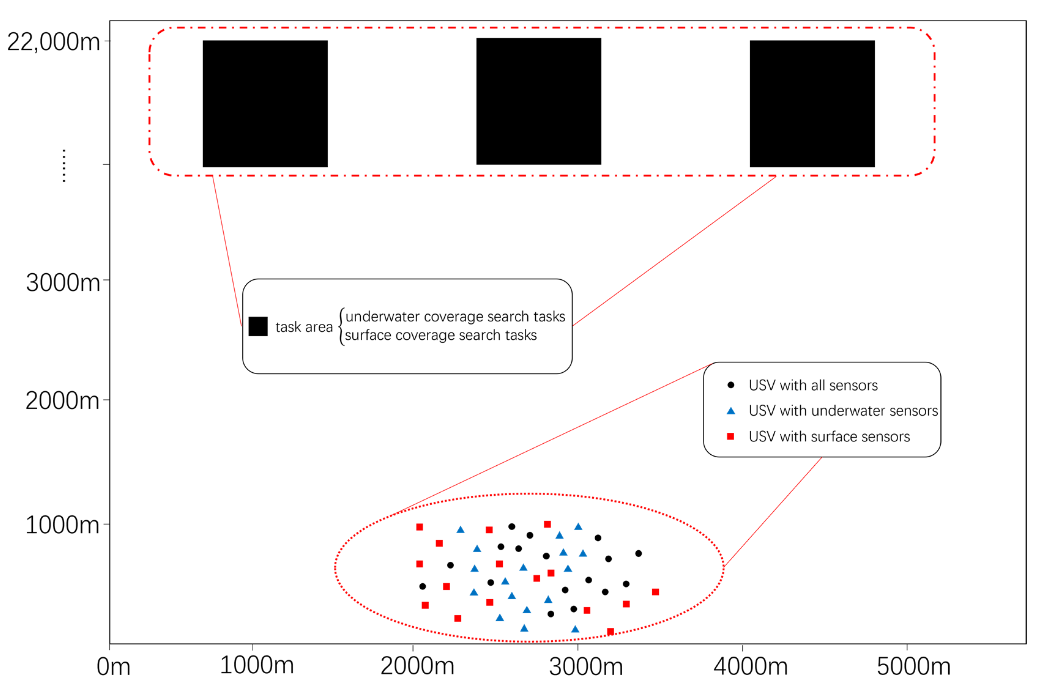
In Figure 1, the operational area of the USVs is confined to a rectangular zone measuring 5000 m by 22,000 m. The red squares represent USVs equipped with surface detection sensors, the blue triangles indicate USVs with underwater detection sensors, and the black dots denote USVs carrying both types of sensors. The black rectangular area at the top represents the mission area, with each USV allocated to a maximum of one mission area for conducting detection tasks. The capabilities of the USVs within the scenario vary, specifically in terms of their maximum sailing speeds (5 m/s to 10 m/s), the types of sensors carried, and their maximum coverage detection speeds (1.4 m/s to 2 m/s). The sensors onboard the USVs are capable of detecting information within a 100 m radius of their location.

At this point, a set of USVs denoted as $U=\left\{u_1,u_2,\dots ,u_{N_u}\right\}$ is present, where $N_u$ represents the number of USVs; $TASK=\left\{tas{k}_1,tas{k}_2,\dots ,tas{k}_{N_t}\right\}$, where $N_t$ denotes the number of target areas. Once the task allocation process for the USVs is completed, they commence their respective missions. While navigating to their task areas and initiating their sensors to conduct searches over the designated regions, the USVs experience energy losses. The ultimate objective of the USV task allocation process is to ensure minimal energy depletion for all USVs while efficiently completing the area search tasks. To assess the quality of the allocation results, this paper introduces a fitness function.

$$fitness=1-\left(w_1\ast \frac{Energy}{Energ{y}_{max}}+w_2\ast \frac{Time}{Tim{e}_{max}}\right).$$

(20)

$Energy$ and $Time$ are terms used to the quantify energy loss and temporal expenditure, respectively, within the context of the allocation scheme. The weighting coefficients $w_1$ and $w_2$ represent the relative importance levels assigned to energy conservation and expedited completion during the task allocation process, respectively. It is stipulated that $w_1+w_2=1$. With the aim of minimizing the total time spent, this study sets $w_1$ to 0.1 and $w_2$ to 0.9. The subsequent sections detail the computational methodologies for determining $Energy$ and $Time$.

$$Energy={\displaystyle \sum }_{i=1}^{Nt}Energ{y}_i.$$

(21)

$$Energ{y}_i=Energ{y}_i^1+Energ{y}_i^2.$$

(22)

$$Energ{y}_i^1={\displaystyle \sum }_{k=1}^3{\displaystyle \sum }_{j=1}^{N_{tk}^i}di{s}_{ij}\ast energ{y}_j^1.$$

(23)

$$Energ{y}_i^2={\displaystyle \sum }_{k=1}^3{\displaystyle \sum }_{j=1}^{N_{tk}^i}lengt{h}_j\ast energ{y}_j^2.$$

(24)

$$Time=ma{x}_{i=1}^{Nt}\left\{Tim{e}_i\right\}.$$

(25)

$$Tim{e}_i=Tim{e}_i^1+Tim{e}_i^2.$$

(26)

$$Tim{e}_i^1=ma{x}_{k=1}^{3}ma{x}_{j=1}^{N_{tk}^i}\frac{di{s}_{ij}}{v_j}.$$

(27)

$$Tim{e}_i^2=max\left\{\frac{Lengt{h}_i^1}{\left({{\displaystyle \sum }}_{j=1}^{N_{u1}^i}{v}_j^{\prime }+{{\displaystyle \sum }}_{j=1}^{N_{u3}^i}{v}_j^{\prime }\right)},\frac{Lengt{h}_i^2}{\left({{\displaystyle \sum }}_{j=1}^{N_{u2}^i}{v}_j^{\prime }+{{\displaystyle \sum }}_{j=1}^{N_{u3}^i}{v}_j^{\prime }\right)}\right\}.$$

(28)

In this context, $Energ{y}_i$ denotes the energy expended by all USVs as they navigate to and execute area search operations within the $i$-th task region. The energy consumed during navigation increases with the number of sensors equipped on each USV. Moreover, the activation of sensors for area search tasks incurs additional energy consumption. The baseline energy consumption for the USVs is quantified as 1 unit per 100 m travelled. For each additional sensor carried or activated for detection purposes, an incremental energy expenditure of 0.03 units per 100 m is incurred.

$Energ{y}_i^1$ and $Energ{y}_i^2$ represent the energy loss induced by all USVs travelling to the $i$-th mission area and the energy loss of each USV performing the search task, respectively. $N_{tk}^i$ represents the number of USVs carrying the $k$-th type of sensor in the $i$-th mission area ($k=1$ for the surface detection sensor, $k=2$ for the submerged detection sensor, and $k=3$ for both types of sensors). $di{s}_{ij}$ represents the distance between the $j$-th USV carrying the $k$-th sensor and the $i$-th mission area. $energ{y}_j^1$ represents the energy loss induced by the USVs during navigation.$lengt{h}_j$ denotes the path length required by the $j$-th USV carrying the $k$-th sensor for area detection. $energ{y}_j^2$ denotes the energy loss induced by the USVs during area detection (when their sensors are activated).

$Tim{e}_i$ denotes the total time spent by all USVs travelling to the $i$-th mission area and performing the coverage search task. $Tim{e}_i^1$ denotes the time consumed by all USVs to travel to the $i$-th target. $v_j$ denotes the maximum navigational speed of the $j$-th USV carrying the $k$-th sensor when travelling to the mission area. $Lengt{h}_i^1$ denotes the total length required for surface sounding in the $i$-th mission area. $Lengt{h}_i^2$ denotes the total length to be covered for underwater detection in the $i$-th mission area. $v_j^{\prime }$ denotes the maximum speed of the $j$-th USV when travelling to the mission area.

In this paper, the quality of the allocation scheme is assessed using the $fitness$ level, which has a value between 0 and 1. A higher value of $fitness$ indicates a better allocation scheme.

To better relate the context of this paper to intelligent algorithms, an example of utilizing the RTPK-SFOA is illustrated. In the task scenario, each task assignment scheme is modelled as a two-dimensional array. In the RTPK-SFOA, the position of each sheep represents a task allocation scheme (a feasible solution), and the fitness of each sheep indicates the quality of the corresponding allocation scheme. The extent of the pasture represents the entire solution space. The goat may be a randomly selected sheep after the initialization of the flock. During the iterative process of the algorithm, the shepherd represents the global optimum solution (the feasible solution with the highest fitness value). For the flock, the speeds of the sheep and the goats are related to the dimensions of the feasible solutions. The specific speed values can be determined according to the specific problem, and an appropriate speed can accelerate the convergence of the algorithm.

To give the reader a better understanding of the variables used in this paper, the variables that appear in the theory section of the algorithm are described in

Table 1. Variable descriptions.

Variables
$r_{Gsheep}$	the grazing radius of the sheep	$P$	the position of the sheep
$r_{Ggoat}$	the grazing radius of the goats	$m,n$	$m\mathrm{th}$/$n\mathrm{th}$ sheep
$upper bound$	the upper limit of the entire grazing area	$i,j$	Row, Column Index
$lower bound$	the lower limit of the entire grazing area	$d$	distance
$T$	time influence factor	$d_1$	hyperparameter
$Iteration$	current number of iterations	$d_2$	hyperparameter
$MaxIteration$	maximum number of iterations	$step$	the moving step size of the sheep
$T_s$	hyperparameter	$\vartheta$	prior knowledge set
$v$	mobility factor	$\vartheta \prime$	secondary prior knowledge set
$C$	hyperparameter		sheep numbering index
$X$	location of an individual	$\mathit{{\rm Y}}$	sheep numbering index
$Dim, dim$	dimensionality of the problem	$\alpha$	sheep numbering index
$Lbest$	the optimal solution	$\beta$	sheep numbering index
$RandomSheep$	a random sheep	$t$	the number of sheep flock breeding iterations
$V$	comprehensive movement factor	$n$	the number of sheep flocks
$T_G$	hyperparameter	$Cof$	the function evaluation cost

.

3.2. Experimental Setup

The CPU used in the experiments of this article is an AMD Ryzen 7 7840HS CPU at 3.80 GHz with 40 GB of memory.

To ensure that the algorithm has good real-time performance and can be applied to practical scenarios, it is specified in this article that the algorithm should run within 120 s and 100 iterations. Based on this, various algorithm parameter settings are determined, as shown in

Table 2. Algorithm parameter settings.

SFOA	PK-SFOA	RTPK-SFOA
Population Size: 200 Number of Goats: 20 Number of Sheep: 180 Goat Step Size: 2 Sheep Step Size: 1	Population Size: 200 Number of Goats: 20 Number of Sheep: 180 The Size of $\vartheta$: 20 Goat Step Size: 2 Sheep Step Size: 1 $d_1$: 2 $d_2$: 2	Population Size: 200 Number of Goats: 20 Number of Sheep: 180 The Size of $\vartheta$: 20 The Size of $\vartheta \prime$: 80 Goat Step Size: 2 Sheep Step Size: 1 $d_1$: 2 $d_2$: 2
WPA	GA	BWO
Population Size: 400 Number of Scout Wolves: 209 Number of Fierce Wolves: 190 Number of Alpha Wolves: 1 Capture Radius: 4 Roaming Step Size: 2 Assault Step Size: 1 Siege Step Size: 1	Population Size: 1000 Cross Probability: 0.44 Mutation probability: 0.01	Population Size: 1000 Reproduction Rate: 0.6 Cannibalism Rate: 0.44 Mutation Rate: 0.4

(for the SFOA, PK-SFOA, RTPK-SFOA, WPA, GA, and BWO).

Experimental Scenario 1: The task is an area search task containing three task areas. The specific attributes are shown in

Table 3. Task scenario attributes.

	$\mathit{t}\mathit{a}\mathit{s}{\mathit{k}}_{\mathit{x}}\left(\mathit{m}\right)$	$\mathit{t}\mathit{a}\mathit{s}{\mathit{k}}_{\mathit{y}}\left(\mathit{m}\right)$	$\mathit{t}\mathit{a}\mathit{s}{\mathit{k}}_{\mathit{a}\mathit{r}\mathit{e}\mathit{a}}\left({\mathit{m}}^2\right)$
Task 1	1000	2000	20,000,000
Task 2	2500	2000	20,000,000
Task 3	4000	2000	20,000,000

.

$tas{k}_x$ represents the $x$-axis coordinate of the bottom centre point of the task area, $tas{k}_y$ represents the $y$-axis coordinate of the bottom centre point of the task area, and $tas{k}_{area}$ represents the size of the task area. All task areas require areas searches both on the surface of the water and underwater. The relevant attributes of the unmanned boats are shown in

Table A1. Attributes of the unmanned boats.

	Ux (m)	Uy (m)	Uv (m/s)	${\mathit{U}}_{\mathit{v}}^{\mathbf{\prime }}$ (m/s)	UProbecategory
USV1	2622	65	5.9	2	1
USV2	2716	56	5.1	2	2
USV3	2131	220	6.9	2	2
USV4	2150	172	5.8	2	2
USV5	2801	352	5.6	2	3
USV6	2287	170	5.6	2	1
USV7	2514	362	6.3	1.7	2
USV8	2441	131	6.7	1.4	2
USV9	2590	243	6.6	2	3
USV10	2190	392	6.7	2	3
USV11	2825	300	5.1	2	2
USV12	2929	44	6.9	1.7	1
USV13	2920	319	7.9	2	1
USV14	2385	239	6.1	2	1
USV15	2033	395	7.8	1.4	1
USV16	2665	26	7.5	1.4	1
USV17	2669	219	6.7	1.4	1
USV18	2131	346	5.6	1.7	2
USV19	2010	305	5.3	1.4	1
USV20	2159	362	6.0	2	1
USV21	2548	381	7.1	2	2
USV22	2712	298	7.2	2	3
USV23	2830	338	5.2	2	1
USV24	2301	91	6.2	1.7	2
USV25	2964	170	7.1	1.7	1
USV26	2993	53	6.7	2	1
USV27	2326	45	7.5	1.4	2
USV28	2253	312	5.2	2	2
USV29	2199	147	6.9	2	2
USV30	2774	291	6.0	2	2
USV31	2125	400	7.4	2	2
USV32	2503	11	5.2	1.4	1
USV33	2894	118	5.4	2	3
USV34	2308	225	6.7	1.7	2
USV35	2519	51	7.6	2	1
USV36	2914	81	5.8	1.7	3
USV37	2874	347	7.8	1.7	3
USV38	2670	123	7.9	2	3
USV39	2712	328	5.8	2	1
USV40	2810	52	6.5	2	2
USV41	2035	164	7.3	2	1
USV42	2997	226	7.3	2	1
USV43	2850	364	7.7	1.4	2
USV44	2614	141	6.2	1.7	2
USV45	2093	207	7.0	1.4	3
USV46	2017	5	5.1	1.7	1
USV47	2281	19	6.6	2	3
USV48	2863	42	6.2	1.4	2
USV49	2390	79	7.7	2	2
USV50	2162	55	5.2	2	1

(located in Appendix A).

$U_x$ represents the $x$-coordinate of the starting point of the unmanned boat, $U_y$ represents the $y$-coordinate of the starting point of the unmanned boat, $U_v$ represents the maximum cruising speed of the unmanned boat towards the task area, $U_v^{\prime }$ represents the maximum cruising speed of the unmanned boat during the area search process, $U_{ProbeCategory}$ represents the type of detection sensor carried by the unmanned boat, $U_{ProbeCategory}=1$ represents that the boat is carrying a surface detection sensor, $U_{ProbeCategory}=2$ represents that the boar is carrying an underwater detection sensor, and $U_{ProbeCategory}=3$ represents that the boat is carrying both types of detection sensors.

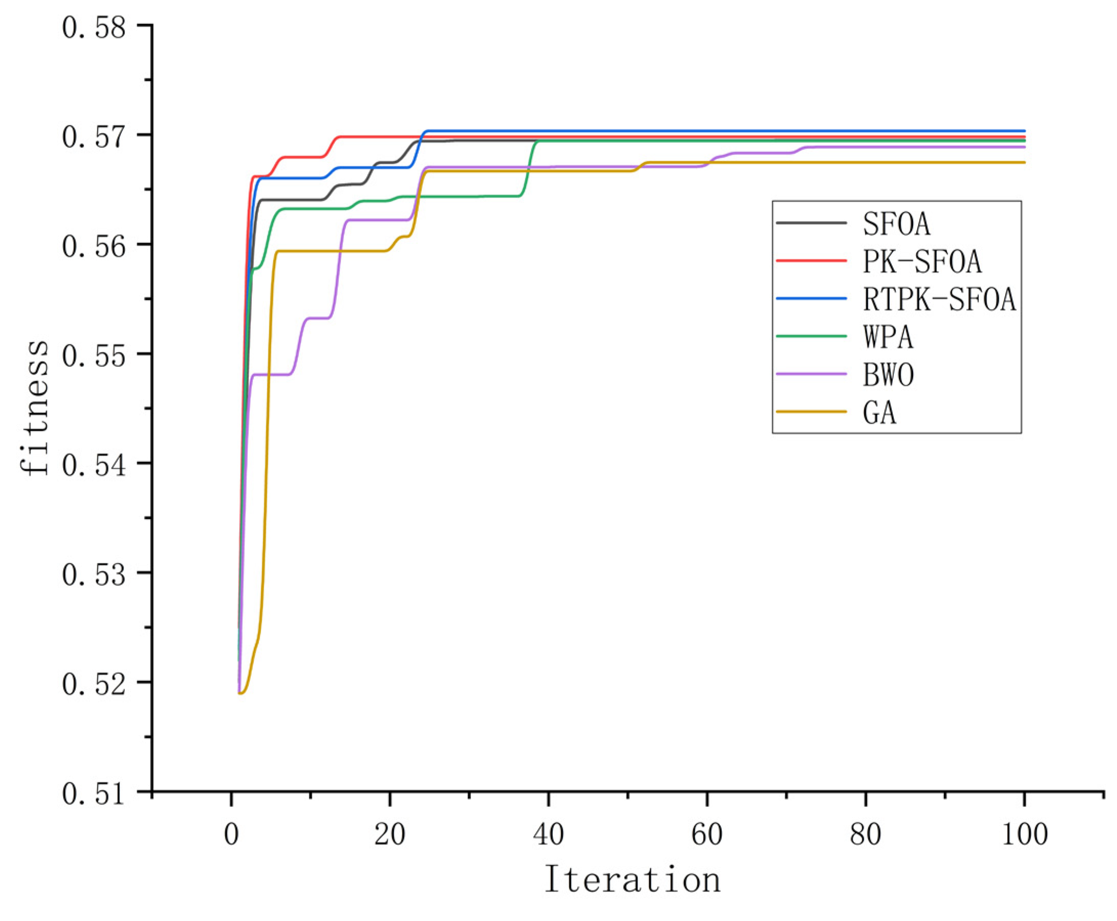
By running various algorithms, algorithm allocation results (

Table A2. Allocation results.

	Task 1	Task 2	Task 3
SFOA	3 7 12 15 17 20 22 27 31 34 38 40 41 42 47 48 50	2 4 5 6 13 14 16 18 21 24 29 33 37 39 45 46	1 8 9 10 11 19 23 25 26 28 30 32 35 36 43 44 49
PK-SFOA	4 6 9 22 25 26 27 28 32 35 37 40 42 44 45 49	2 3 10 12 13 14 17 18 19 23 24 31 33 34 36 43 50	1 5 7 8 11 15 16 20 21 29 30 38 39 41 46 47 48
RTPK-SFOA	3 5 6 8 9 16 19 21 24 27 30 38 39 42 44 46 50	1 11 14 22 25 26 28 31 32 33 37 40 41 45 48 49	2 4 7 10 12 13 15 17 18 20 23 29 34 35 36 43 47
WPA	6 7 9 13 16 18 21 23 27 35 36 38 40 42 44	1 2 10 11 14 17 20 22 26 28 29 30 32 46 47 48 50	3 4 5 8 12 15 19 24 25 31 33 34 37 39 41 43 45 49
GA	3 7 9 16 19 23 24 26 28 31 33 37 40 42 43 46 50	1 5 8 15 17 20 25 29 30 34 35 38 44 45 47 49	2 4 6 10 11 12 13 14 18 21 22 27 32 36 39 41 48
BWO	1 4 5 6 9 16 17 18 24 26 27 28 31 34 41 46 47	8 11 14 20 21 22 23 25 29 32 33 35 37 40 44 45	2 3 7 10 12 13 15 19 30 36 38 39 42 43 48 49 50

(located in Appendix A)) and a schematic diagram of the iteration process are obtained (Figure 2). The fitness values in Figure 2 are capable of assessing the quality of the tested allocation schemes. A higher fitness value indicates that the corresponding allocation scheme enables the USVs to complete tasks in a shorter period with less energy expenditure. In Figure 2, the larger the fitness value at the convergence time of an algorithm, the better the allocation scheme obtained by that algorithm.

According to Figure 2, compared to the SFOA [9], due to the presence of prior knowledge, the PK-SFOA can better escape from local optima and achieve better convergence. Compared to the PK-SFOA, the RTPK-SFOA introduces an updating mechanism based on prior knowledge, which enhances its ability to escape local optima and guide the population towards the optimal solution. Moreover, the RTPK-SFOA outperforms other algorithms, such as the GA [7], BWO [11], and WPA [10], in terms of the optimization effect.

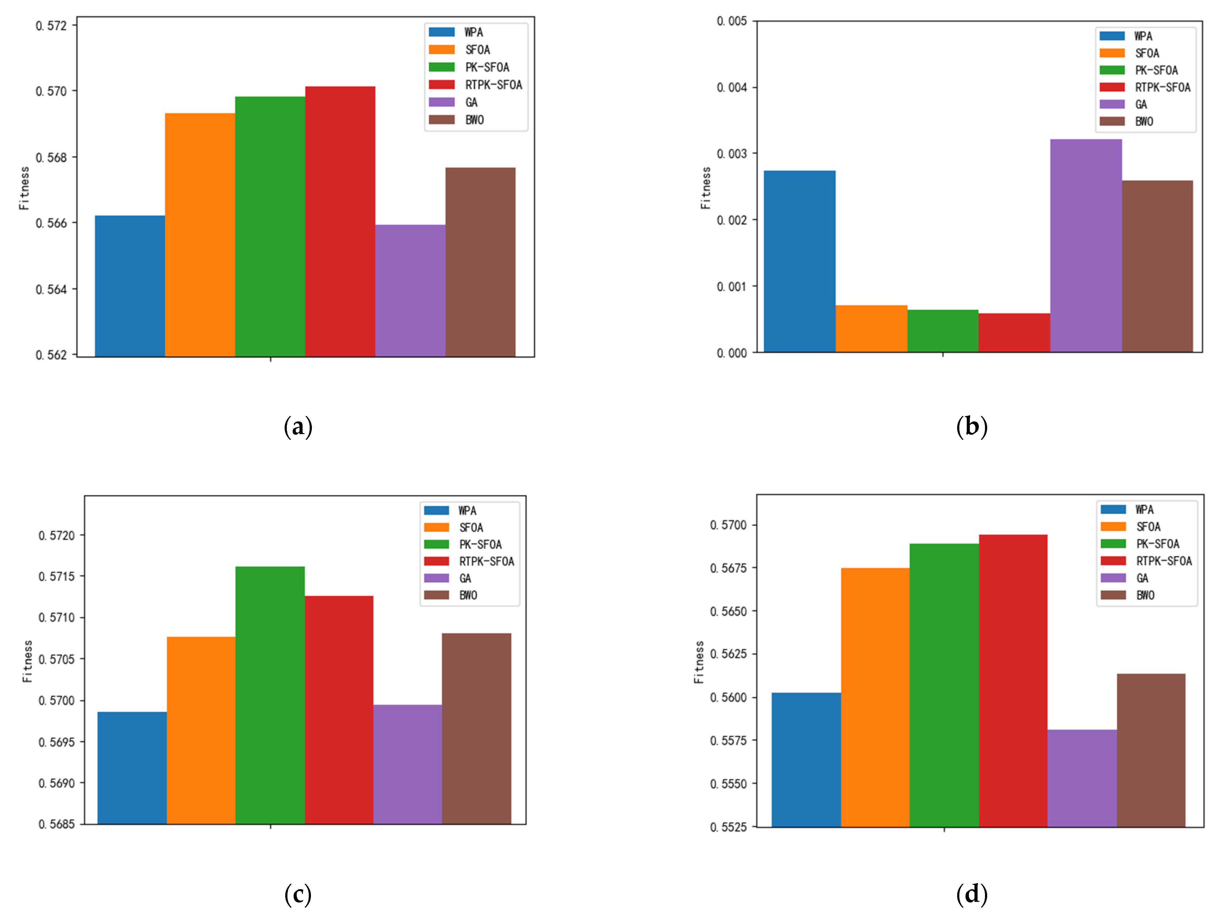
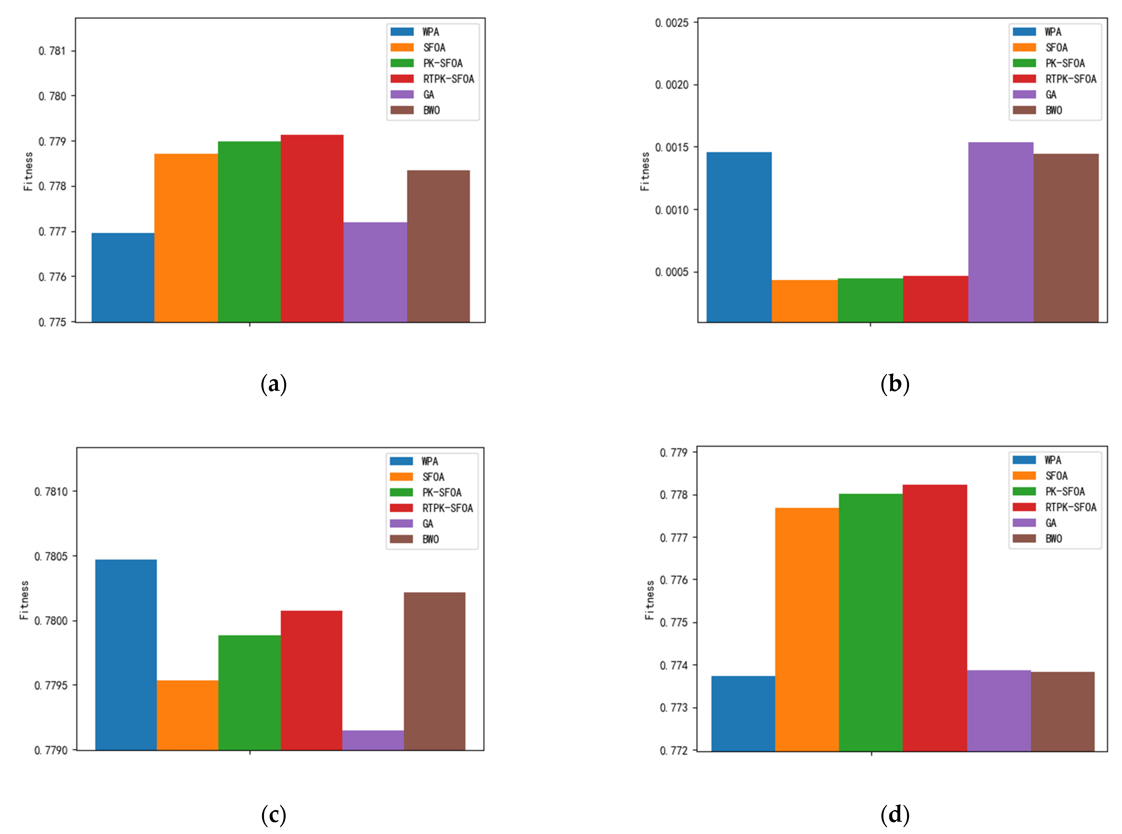
Due to the random nature of intelligent algorithms, this paper runs the various algorithms 30 times against the background of experimental scenario 1 and statistically analyses the final results, as shown in Figure 3. In Figure 3, the mean values represent the average fitness levels of the algorithms after 30 runs, which represent the average performance of the algorithms. The best and worst values are the best (upper limit) and worst (lower limit) fitness values produced by the algorithms after 30 runs, respectively, and the Std values are the standard deviations of the fitness levels of the algorithms after 30 repeated runs; the smaller a value is, the more stable the corresponding algorithm is.

As shown in Figure 3, the PK-SFOA with a priori knowledge significantly improves the mean fitness, best fitness and worst fitness values over those of the SFOA [9]. This is because the a priori knowledge helps to prevent the algorithm from falling into a local optimum. However, since the a priori knowledge is not updated, underexplored regions may be located near the a priori knowledge set, which may result in the algorithm failing to find the optimal solution if the optimal solution occurs in that region. Compared with the PK-SFOA, the RTPK-SFOA updates the a priori knowledge set to better explore the previously underexplored regions. As a result, the RTPK-SFOA obtains better mean fitness and worst fitness values than those of the PK-SFOA. Figure 3a,b show that the RTPK-SFOA has a greater mean fitness and a lower standard deviation value than those of the SFOA, PK-SFOA, GA [7], BWO [11] and WPA [10]. This indicates that the RTPK-SFOA is more stable and able to obtain better allocation schemes in a shorter period.

Due to the presence of both prior and candidate prior knowledge sets in the RTPK-SFOA, the algorithm effectively reduces the probability of falling into a local optimum. As a result, compared to all other algorithms, the RTPK-SFOA has a higher mean (indicating better performance) and a smaller standard deviation (indicating greater stability). However, the disadvantage of the RTPK-SFOA is that it requires more computational resources and has a longer computation time than the other algorithms.

To prove that the improved algorithm proposed in this paper performs well in different experimental scenarios, the location and size of the task area are modified, and a new task scenario 2 is constructed for testing (the relevant information concerning the USVs remains unchanged).

Experimental Scenario 2: The task area properties are reset (The specific attributes are shown in

Table 4. Task scenario attributes.

	$\mathit{t}\mathit{a}\mathit{s}{\mathit{k}}_{\mathit{x}}\left(\mathit{m}\right)$	$\mathit{t}\mathit{a}\mathit{s}{\mathit{k}}_{\mathit{y}}\left(\mathit{m}\right)$	$\mathit{t}\mathit{a}\mathit{s}{\mathit{k}}_{\mathit{a}\mathit{r}\mathit{e}\mathit{a}}\left({\mathit{m}}^2\right)$
Task 1	1000	1500	10,000,000
Task 2	2500	1500	10,000,000
Task 3	4000	1500	10,000,000

).

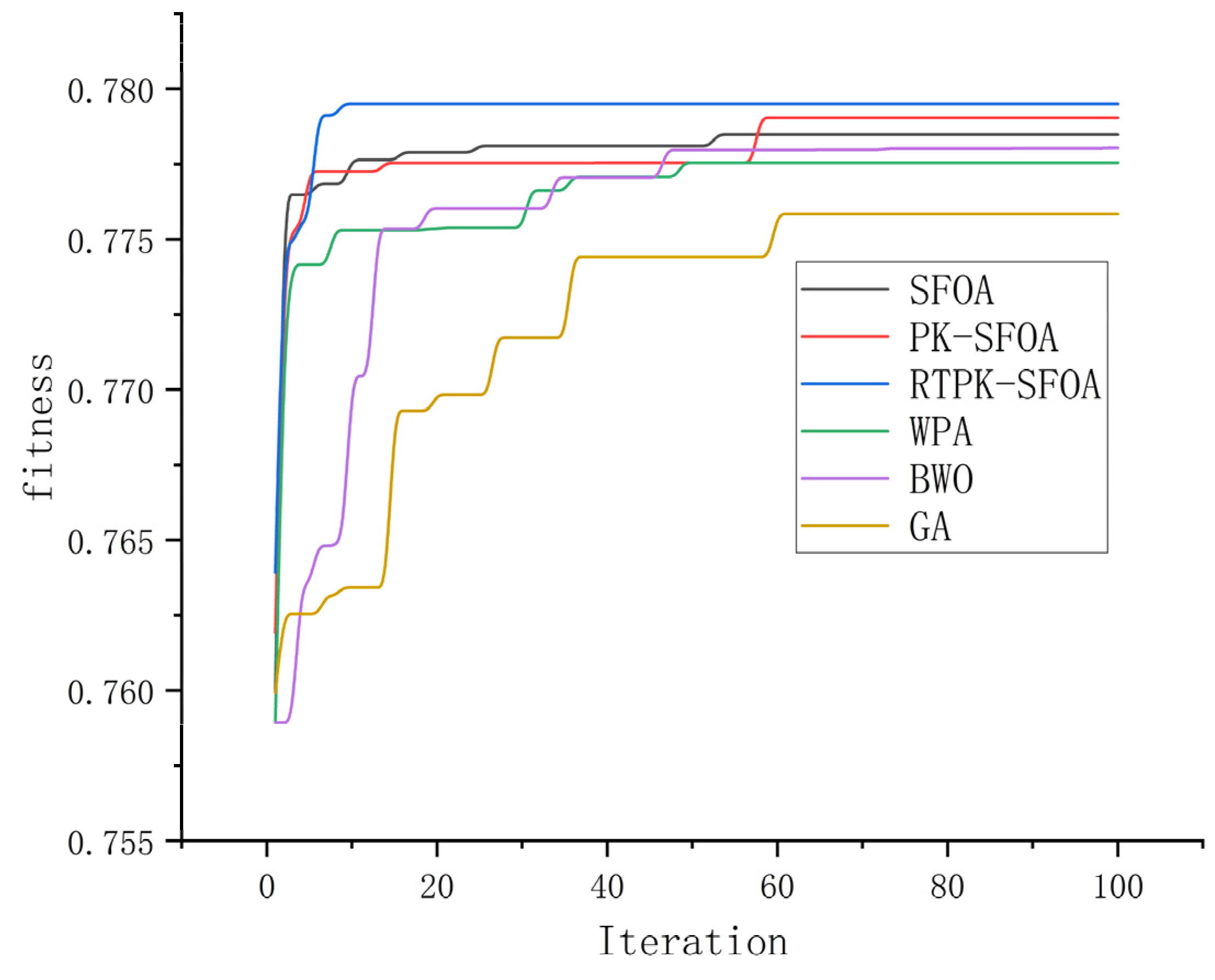
Various algorithms are run to obtain algorithmic assignment results (

Table A3. Allocation results.

	Task 1	Task 2	Task 3
SFOA	1 10 11 12 13 14 21 22 24 30 32 34 36 40 43 46 50	2 7 17 18 19 23 25 26 27 28 33 35 37 39 44 47 49	3 4 5 6 8 9 15 16 20 29 31 38 41 42 45 48
PK-SFOA	3 4 5 8 12 13 15 21 27 31 35 37 38 41 42 46 49	1 6 9 16 17 22 23 24 25 26 28 29 34 40 43 44 45	2 7 10 11 14 18 19 20 30 32 33 36 39 47 48 50
RTPK-SFOA	3 4 12 13 18 19 22 26 27 28 33 35 44 46 47 49 50	1 2 5 6 8 11 15 17 20 23 24 30 32 34 36 38 43	7 9 10 14 16 21 25 29 31 37 39 40 41 42 45 48
WPA	9 11 15 18 19 20 28 33 34 35 44 48 49 50	1 2 6 8 13 17 21 22 24 25 26 31 32 36 38 45 46 47	3 4 5 7 10 12 14 16 23 27 29 30 37 39 40 41 42 43
GA	3 7 8 14 16 17 20 22 23 27 28 30 33 34 35 36 41 43	1 2 5 9 11 15 19 21 31 32 38 39 44 46 49 50	4 6 10 12 13 18 24 25 26 29 37 40 42 45 47 48
BWO	3 5 7 9 14 16 17 21 27 31 34 35 38 39 42 49 50	4 11 12 13 18 19 24 25 26 29 33 41 43 44 45 46 47	1 2 6 8 10 15 20 22 23 28 30 32 36 37 40 48

(located in Appendix A)), and a schematic diagram of the iteration process is shown in Figure 4.

According to Figure 4, the PK-SFOA outperforms the SFOA, and the final fitness of the PK-SFOA is greater than that of the SFOA because the PK-SFOA introduces an a priori knowledge set. Since the RTPK-SFOA introduces a set of prior knowledge and a set of candidate prior knowledge, which reduces the probability of the algorithm falling into a local optimal solution, the RTPK-SFOA converges faster and has the highest adaptability.

Due to the random nature of the intelligent algorithms, to verify the average performance of the algorithms, this paper runs each algorithm 30 times in Scenario 2 and statistically analyses their final results. The results are shown in Figure 5.

After changing the task scenario, it can be seen from Figure 5a,b that compared with other algorithms, the RTPK-SFOA has a smaller standard deviation, the highest average adaptation, and better performance. Figure 5b–d show that although the best adaptations of the WPA [10] and BWO [11] are better than those of the RTPK-SFOA proposed in this paper, their worst adaptations are lower, and their standard deviations are larger, which indicates that these algorithms are less stable and cannot guarantee the acquisition of the optimal solution in a short period.

The experimental part of this paper simulates real task scenarios and proves that the RTPK-SFOA has good performance and stability. However, compared with other algorithms, the RTPK-SFOA needs more parameters to be defined and requires more computational resources. In real-world applications, if the CPU performance at the control centre is inferior, extended durations might be needed to obtain allocation results.

4. Conclusions

Currently, the mainstream approach for solving the task allocation problem of heterogeneous multi-unmanned systems is to utilize intelligent algorithms. However, many intelligent algorithms fail to make full use of population information, resulting in poor global optimization capabilities. To address this problem, this paper utilizes the information eliminated from a population to establish a set of a priori knowledge, which provides a reference for the reproduction of the population and ultimately forms a task allocation algorithm based on real-time a priori knowledge updates. To verify the superiority of the algorithm proposed in this paper, two task scenarios are constructed, and ablation experiments are conducted. Figure 3a,b and Figure 5a,b show that the improved algorithm proposed in this paper performs better (with a higher mean) and more stably (with a smaller standard deviation) than the other tested algorithms. It is proven that the improved algorithm (the RTPK-SFOA) proposed in this paper can effectively combine the parameters of USVs and mission area information and reasonably carry out the cooperative task allocation process.

The RTPK-SFOA proposed in this paper requires a greater computational load than the SFOA. If the parameters in the RTPK-SFOA are not properly configured, the performance of the algorithm can be greatly reduced. In addition, although the RTPK-SFOA can run on low-end hardware, a population that is too large or a task that is too complex can result in long run times. Future research directions will include designing a strategy to reduce the computational effort required by the RTPK-SFOA while keeping its optimization capabilities intact to ensure that the algorithm can compute quickly on low-end hardware.