Abstract
Traffic flow prediction is considered to be one of the fundamental technologies in intelligent transportation systems (ITSs) with a tremendous application prospect. Unlike traditional time series analysis tasks, the key challenge in traffic flow prediction lies in effectively modelling the highly complex and dynamic spatiotemporal dependencies within the traffic data. In recent years, researchers have proposed various methods to enhance the accuracy of traffic flow prediction, but certain issues still persist. For instance, some methods rely on specific static assumptions, failing to adequately simulate the dynamic changes in the data, thus limiting their modelling capacity. On the other hand, some approaches inadequately capture the spatiotemporal dependencies, resulting in the omission of crucial information and leading to unsatisfactory prediction outcomes. To address these challenges, this paper proposes a model called the Dynamic Spatial–Temporal Self-Attention Network (DSTSAN). Firstly, this research enhances the interaction between different dimension features in the traffic data through a feature augmentation module, thereby improving the model’s representational capacity. Subsequently, the current investigation introduces two masking matrices: one captures local spatial dependencies and the other captures global spatial dependencies, based on the spatial self-attention module. Finally, the methodology employs a temporal self-attention module to capture and integrate the dynamic temporal dependencies of traffic data. We designed experiments using historical data from the previous hour to predict traffic flow conditions in the hour ahead, and the experiments were extensively compared to the DSTSAN model, with 11 baseline methods using four real-world datasets. The results demonstrate the effectiveness and superiority of the proposed approach.
1. Introduction
With the rapid development and breakthroughs in technologies such as the Internet of Things (IoT), digital communication, artificial intelligence, and big data mining, the process of urban smartification continues to advance. Intelligent transportation systems (ITSs) [1,2,3,4,5], as an integral part of smart city development, play a crucial role in managing, analysing, optimising, and improving urban traffic conditions. Among the core technologies of ITSs, traffic flow prediction [6,7,8,9] aims to forecast the future traffic conditions for a certain period of time based on the historical traffic data collected from sensors in the road traffic network [10,11,12,13,14,15]. This prediction capability is essential for proactive traffic management, real-time route planning, congestion mitigation, and the overall improvement of urban mobility.
Different from traditional time series analysis tasks, traffic flow prediction not only requires considering temporal and spatial dependencies at multiple scales [16], but it is also susceptible to external factors such as weather conditions, unexpected events, and people’s travel habits, exhibiting unstable conditions. Moreover, traffic conditions exhibit significant periodic patterns, such as weekdays and weekends, as well as differences in traffic conditions between peak and off-peak hours. Therefore, how to predict the traffic flow situation in real time and accurately is of great significance to reduce traffic congestion, improve the urban traffic environment, and enhance the quality of life of residents.
As an early solution for traffic flow prediction, initial work employed queuing theory to simulate traffic behaviours [17,18]. However, such methods lacked sufficient consideration of the highly complex correlations present in the traffic data. Subsequently, some studies abstracted the traffic flow prediction problem as a simple time series forecasting task and attempted to combine various statistical methods in search of effective solutions [19,20]. However, most of these methods required traffic data to satisfy specific assumptions, which rendered them ineffective in addressing complex issues such as nonlinearities and dynamic spatiotemporal dependencies in the data. As a result, the prediction outcomes often fell short of expectations. Later on, machine learning-based approaches [21,22] emerged, which were capable of capturing the complex nonlinear features in the traffic data. However, these methods overly relied on manual feature engineering during the processing stage, making it challenging to effectively incorporate the dynamic spatiotemporal correlations within the data. Consequently, the modelling capabilities of these methods were limited, and the prediction results remained unsatisfactory.
In recent years, with the development of deep neural network models, some works [4,23,24,25] have proposed the use of Recurrent Neural Networks (RNNs) and their variants, such as Long Short-Term Memory (LSTM) [26] and Gated Recurrent Units (GRUs) [20,27], to capture the dynamic spatiotemporal dependencies in the traffic data, or combined the attention mechanisms [28,29] with RNN models to improve the fusion efficiency of dynamic spatiotemporal dependencies in the data. Additionally, some works [2,30,31,32] have introduced Convolutional Neural Networks (CNNs) [33] to model the spatial correlations in the traffic data. Subsequently, Graph Neural Network (GNN) models [34,35,36] have emerged as popular solutions for traffic flow prediction tasks due to their natural suitability for handling non-Euclidean data with high-dimensional spatial structures and their ability to capture complex spatiotemporal features and correlations in the traffic data, and have garnered widespread attention and research interest [2,4,37,38,39,40,41]. However, despite the fruitful achievements and the significant advancement they have brought to the field of traffic prediction, these methods still inevitably face the following issues:
- (1)
- Insufficient modelling of spatial dependencies in traffic flow data.
The traffic flow reflects the daily travel patterns of residents, providing insights into their commuting habits. Traffic conditions are influenced by the diverse functional areas within a city, including residential areas, industrial parks, and commercial districts. It is observed that adjacent regions with different functions, such as industrial parks and residential areas, exhibit noticeable disparities in traffic conditions. Conversely, geographically distant areas with similar functions, such as commercial districts, tend to have comparable traffic conditions. However, most existing methods primarily focus on the local spatial correlations based on the topological structure of the road network, while neglecting the inherent global spatial dependencies in traffic flow data;
- (2)
- Insufficient modelling of the dynamic spatial–temporal correlations in the traffic data.
Unlike the stable propagation of information in information networks, traffic flow states are highly susceptible to the influence of weather conditions and unexpected events, resulting in highly dynamic variations. Most existing research heavily relies on specific static assumptions, such as predefined static adjacency matrices, which severely restrict the modelling capacity and lead to the loss of many pieces of crucial dynamic spatiotemporal correlation information in the traffic data. Consequently, accurately capturing the true dynamic characteristics of spatiotemporal dependencies in the traffic data becomes challenging.
To solve the above problems, this paper proposes a new model called the Dynamic Spatial–Temporal Self-Attention Network (DSTSAN). The model utilises a feature augmentation module to amplify the information interaction among different dimensions of features, thereby enhancing the representation capacity of the model. Subsequently, the spatial self-attention module and two masking matrices are employed to adequately model the local and global spatial dependencies in the traffic data. Finally, a temporal self-attention module is used to capture the dynamic patterns in the data and effectively fuse them with the spatial dependency features.
In summary, the main contributions can be summarised as follows:
- (1)
- This research proposed a new Dynamic Spatial–Temporal Self-Attention Network to solve the problem of insufficient dynamic spatial–temporal correlation modelling in the traffic flow prediction process;
- (2)
- Building upon the spatial self-attention mechanism, this methodology introduces two masking matrices to model the local and global spatial correlations in the data, respectively. Furthermore, a temporal self-attention module is employed to integrate dynamic temporal dependencies, thereby achieving effective modelling of the dynamic spatiotemporal dependencies in the traffic data;
- (3)
- The current investigation conducted extensive comparative experiments with 11 baseline methods on four real datasets. The experimental results demonstrate the validity and superiority of this model.
This paper is organised as follows: Section 2 covers related works. Section 3 mainly explains and formally defines the relevant concepts and problems. In Section 4, this research provides a detailed description of the proposed DSTSAN model. And Section 5 conducts extensive comparative experiments between the DSTSAN model and 11 baseline methods on four publicly available real-world datasets, and the experimental results are thoroughly analysed. Additionally, ablation studies and parameter sensitivity analysis are conducted in this section. Section 6 summarises and concludes the research conducted in this paper.
2. Related Work
2.1. Graph Convolution Network
Graph Convolutional Neural Networks (GCNs) [42,43] are an extension of Convolutional Neural Networks (CNNs) applied to non-Euclidean spatial data represented by graph structures. They can be categorised into spectral domain graph convolution networks and spatial domain graph convolution networks [14,44,45,46,47,48]. The spectral domain approach extends the Convolutional Neural Network algorithm to process graph-structured data by utilising the graph Laplacian matrix, which resembles the Fourier transform in signal processing. However, computing all the eigenvalues of the graph Laplacian matrix introduces high computational complexity. To address this, ChebNet [43] replaces the convolutional kernel in spectral domain graph convolution with Chebyshev polynomials, resulting in significant efficiency improvements. Building upon ChebNet, the classical GCN [42] further simplifies the model by employing a first-order Chebyshev polynomial as an approximation of the ChebNet filter. Consequently, the classical GCN is regarded as a first-order approximation model of ChebNet.
Spatial domain graph convolution networks are defined based on the mechanism of information propagation [48]. For example, Message Passing Neural Networks (MPNNs) [49] utilise message passing functions to unify different variants in the spatial domain. In GraphSAGE [50] and Diffusion Graph Convolutional Networks (DGCs) [51], the graph convolution operation is modelled as a process of diffusion or direct information propagation from a node to its adjacent nodes with a certain probability. Graph Attention Networks (GATs) [52] employ attention mechanisms to learn the relative weights between adjacent nodes, and incorporate the attention mechanism into the information propagation process. Moreover, GAT utilises multi-head attention mechanisms to ensure stable learning.
2.2. Attention Mechanism
The attention mechanism is a method inspired by the human visual and cognitive systems, enabling models to learn automatically and selectively focus on the most crucial information in the input data for the current task, thereby enhancing the model’s performance and generalisation ability. In multitask processing, attention mechanisms exhibit excellent capability in capturing long-range dependencies and have found widespread applications in natural language processing (NLP), speech recognition (ASR), machine translation (MT), computer vision (CV), and other domains. Among recent notable attention models, GMAN [29] employs a multi-level attention mechanism to dynamically adjust the correlations between different geographical sensors in temporal prediction tasks. However, this approach requires setting up a separate model at each time step, resulting in high computational complexity. GAT [52] utilises a self-attention mechanism to compute attention weights between the central node and its adjacent nodes, capturing local spatial dependencies of the central node. Transformer [53] employs a self-attention mechanism to facilitate the propagation of temporal information, addressing the challenge of capturing long-range dependencies in multitask processing that traditional Recurrent Neural Networks (RNNs) and Convolutional Neural Networks (CNNs) struggle with. However, Transformer is computationally expensive and is not suitable for large-scale long sequence prediction tasks. Subsequently, Informer [54], based on the Transformer architecture, replaces the dot-product attention mechanism with the ProbSparse self-attention mechanism, significantly alleviating the computational cost issue in long sequence prediction tasks.
2.3. Traffic Flow Prediction
Traffic flow prediction, originally originated from the task of univariate time series forecasting, has evolved into a typical case of multivariate time series forecasting [45,55]. Early research on traffic flow prediction was mainly based on statistical models, with classical methods including Vector Autoregression (VAR) [56], Kalman filtering [19], Autoregressive Integrated Moving Average (ARIMA) [57], and so on. These methods were primarily linear and based on specific static assumptions, making them unable to handle complex and highly nonlinear traffic data. Subsequently, classical machine learning methods such as Support Vector Regression (SVR) [21] and XGBoost [22] were proposed. Although these methods could effectively capture the nonlinear features in the traffic data, they heavily relied on manually designed feature engineering, limiting the models’ feature processing capabilities. In recent years, deep neural networks have dominated the field of traffic flow prediction due to their efficient modelling capabilities for complex nonlinear features in spatial–temporal data [45]. The most common methods are based on Recurrent Neural Networks (RNNs) and Convolutional Neural Networks (CNNs). DCRNN [4] and GRUED [27] both adopt an encoder–decoder architecture. The former utilises Diffusion Graph Convolutional Networks (GCNs) [4] and random walk to describe the spatial dependencies in the traffic data, while incorporating pre-sampling techniques to capture dynamic temporal features. The latter deeply integrates the encoder–decoder architecture with the GRU model and performs traffic flow prediction through temporal modelling. DSANet [58] utilises two CNN modules to model local and global temporal dependencies, and then integrates spatial correlations using self-attention mechanisms. However, CNN-based methods often combine one-dimensional spatial–temporal convolutions with graph convolutions [2], which results in a complex model due to the need for stacking multiple layers to expand the receptive field. Graph Convolutional Neural Networks (GCNs), on the other hand, have inherent advantages in modelling high-dimensional spatiotemporal data, allowing for a better fit to the complex spatiotemporal dependencies inherent in the traffic data. STGCN [2] and ASTGCN [29] both employ graph convolution (GCN) modules and Convolutional Neural Networks (CNNs) to model spatial and temporal dependencies, respectively. Graph WaveNet [37] was the first to use two learnable embedding matrices to automatically construct adaptive graphs, enabling the efficient modelling of spatiotemporal correlations in the traffic data. FOGS [10] addresses the issue of insufficient fitting in traffic prediction by utilising first-order gradient training models. D2STGNN [11] designs a spatiotemporal decoupling framework to separate diffusion signals and intrinsic signals hidden in the traffic data, aiming for the accurate modelling of traffic data. PDFormer [13] introduces two graph mask matrices to model local and global spatial correlations, and then combines them with temporal dynamic dependencies using spatial self-attention mechanisms.
In addition to the aforementioned methods, other approaches such as differential equations [59,60], spatial–temporal graph neural point processes [61], and Dynamic Time Warping (DTW) [62] have also been used to improve traffic flow prediction and have achieved a series of remarkable results. These methods provide new insights into modelling the dynamic spatiotemporal correlations in the traffic data and have contributed to the vibrant development of the field of traffic prediction.
3. Preliminaries
In this subsection, a brief description of the important concepts is introduced and the problems are addressed, as well as a formal definition of them:
Traffic sensors are sensors deployed at various intersections on the traffic network to record and collect information such as traffic flow and speed.
The road traffic network is the traffic network formed by intersecting urban roads. Intersections are regarded as nodes in the traffic network, and urban roads connecting two nodes are regarded as edges in the traffic network.
Definition 1.
(Road Traffic Network): This model defines the road traffic network as a traffic network or a traffic graph, denoted as , where is a finite set of nodes in the graph , with , where is the total number of nodes in the graph , corresponding to traffic sensors deployed at various locations in the traffic network. represents the set of edges in the traffic graph . is the adjacency matrix of the traffic graph . For any node in the traffic graph , if there is an edge connecting node and node , then , otherwise ..
Traffic signals refer to the actual traffic flow measurements recorded by all traffic sensors in a traffic network at a given time step.
Definition 2.
(Traffic Signal): The traffic signal , represents the measurement values of all the sensors in the traffic graph at time . denotes the feature dimension of the traffic information such as vehicle speed, traffic volume, etc. represents the total number of nodes in the traffic graph .
Traffic flow prediction refers to the process of predicting the traffic conditions in a road network for a future period based on the traffic data collected by sensors deployed in the network over a certain historical time interval.
Problem Definition
(Traffic Flow Prediction): Given a traffic graph and traffic signals within consecutive historical time steps, t’s objective is to learn a mapping function that accurately predicts the traffic flow conditions of graph for the next consecutive time steps:
4. Methodology
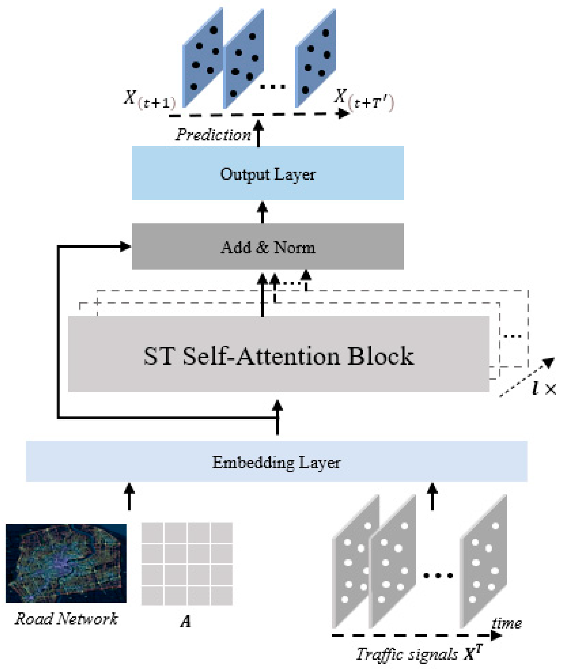
This research has developed a novel model called the Dynamic Spatial–Temporal Self-Attention Network (DSTSAN), which is depicted in Figure 1. The DSTSAN model comprises three main layers: the feature embedding layer, the spatial–temporal self-attention layer, and the output layer. The spatial–temporal self-attention layer is constructed by connecting self-attention modules in parallel. In the subsequent sections, this paper will provide a comprehensive description of each component in the DSTSAN model.
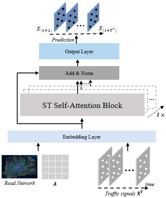
Figure 1.
The overall framework of DSTSAN.
4.1. Embedding Layer
The embedding layer is primarily composed of a fully connected network, which converts the input data into a shared high-dimensional representation space, thereby facilitating further processing and analysis.
Firstly, the traffic signal is converted and the traffic network adjacency matrix is converted into vector representations, resulting in converted signal vectors and . Here, represents the historical time steps, denotes the total number of nodes in the traffic network, and represents the embedding dimension. To effectively capture the weekly periodicity (distinguishing weekdays from weekends), two embedding matrices are introduced for time periods: and . represents the number of time slots in a day, determined by the data collection frequency of traffic sensors, and represents the number of days in a week (). This implies that the same time slot within a day and the corresponding time slot on the same day of the week share the same time period embedding. By concatenating the periodic embedding vectors of time steps, the daily periodicity embedding vector is obtained, and the weekly periodicity embedding vector . Finally, this method concatenates the aforementioned embedding vectors to obtain the output of the embedding layer:
where is the concatenate operation.
4.2. Spatial–Temporal Self-Attention Layer
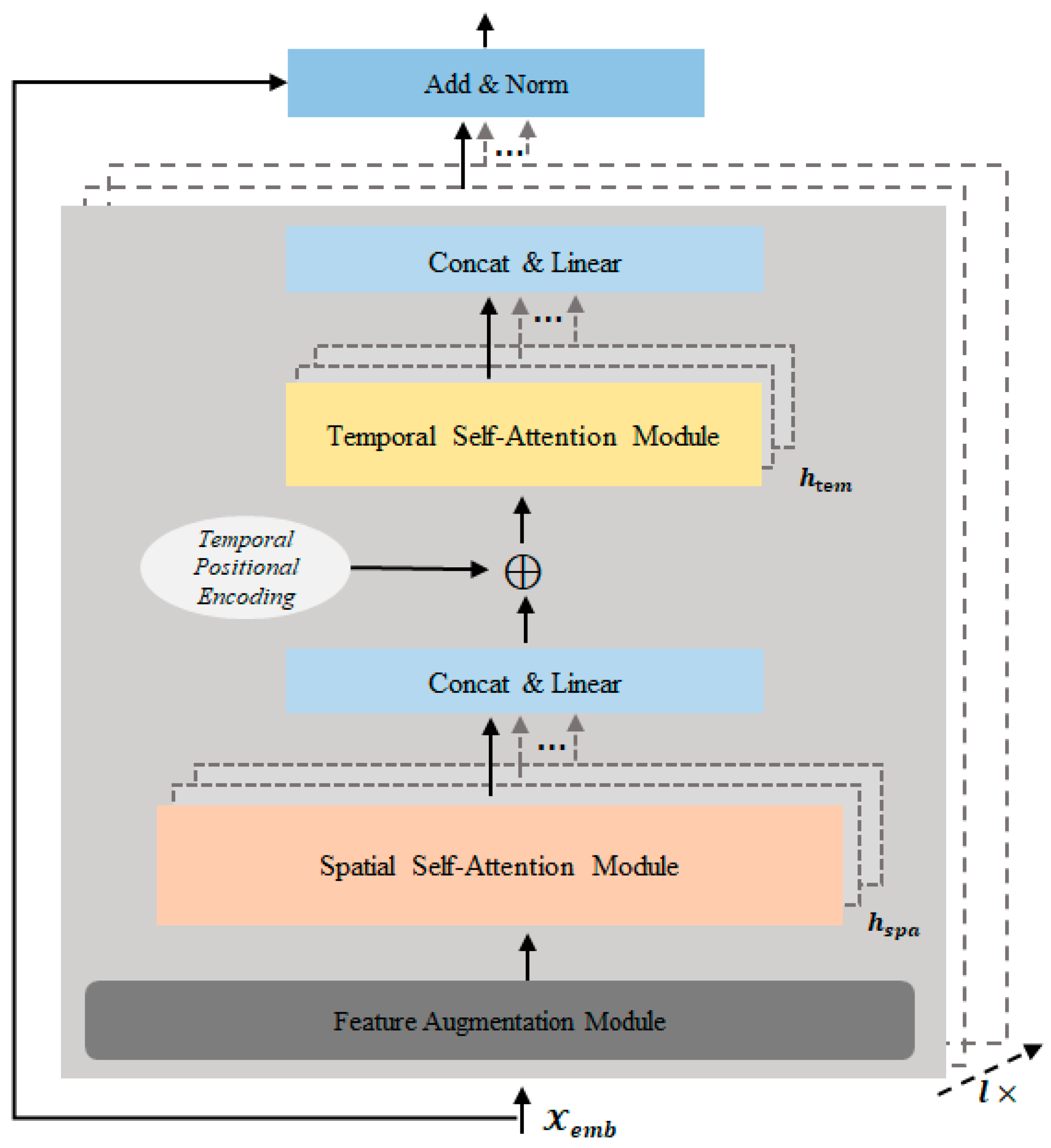
In order to capture the intricate dynamic spatiotemporal dependencies in the traffic data, this research has devised a spatial–temporal self-attention layer, as illustrated in Figure 2. This layer employs residual connections and comprises self-attention modules that are connected in parallel. Each self-attention module consists of key components, including the feature augmentation module, spatial self-attention module, and temporal self-attention module.
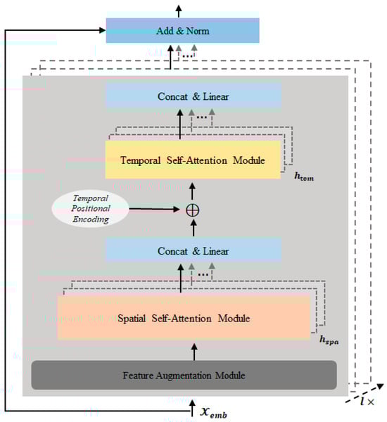
Figure 2.
Spatial–temporal self-attention layer.
4.2.1. Feature Augmentation Module
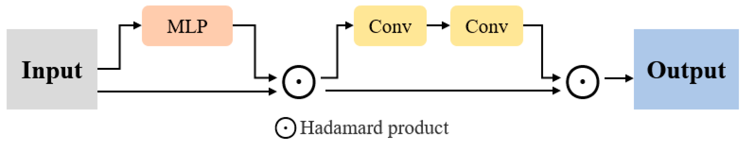
Traffic data are highly complex, and different features have varying influences on the traffic flow. In order to comprehensively model the intrinsic correlations among the features in the traffic data, inspired by the channel attention mechanism [63], this research utilises a feature augmentation module to enhance the interactions between different feature dimensions of the traffic data. This enables the model to learn the importance of different feature dimensions automatically.
Figure 3 depicts the schematic diagram of the feature augmentation module. The input data are compressed using a multilayer perceptron (MLP) with a single hidden layer. Then, a single activation process is applied to determine the importance and correlation of each feature dimension with respect to the crucial information. Subsequently, the temporal features of the traffic data are enhanced through the concatenation of two one-dimensional convolutions. This process strengthens the interaction of information in the traffic data across both spatial and temporal dimensions.

Figure 3.
The feature augmentation module.
Given the embedding vector of the input data, the feature augmentation process is formally represented as follows:
where ⊙ denotes the Hadamard product, is the activation function, and is the activation function, , are the learnable weight parameter matrix and bias matrix, respectively, is the convolution kernel, and denotes the convolution operation. represents the time step and denotes the dimensions of .
4.2.2. Spatial Self-Attention Module
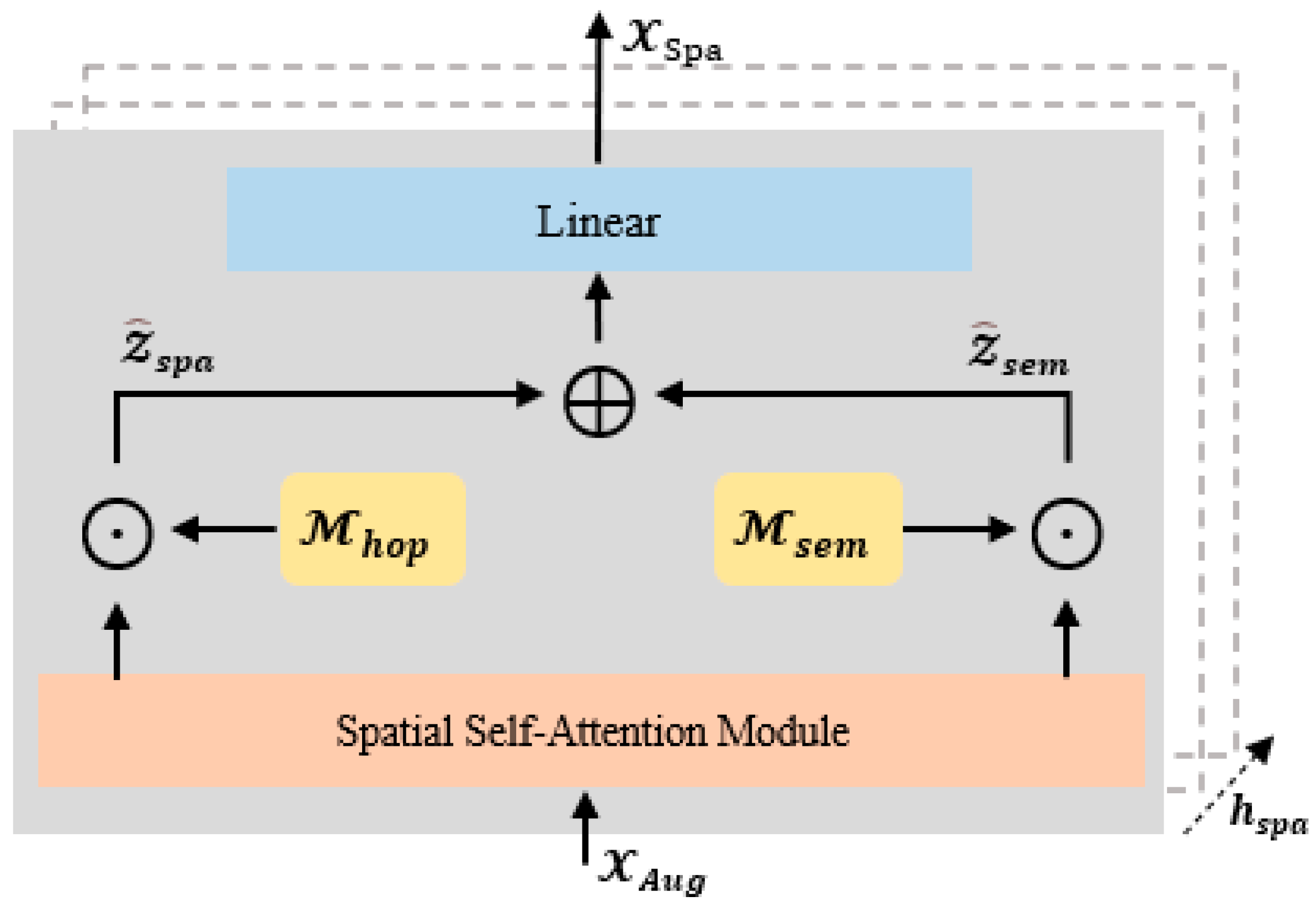
Traffic data exhibit complex spatial correlations, encompassing both local spatial dependencies, such as the traffic conditions at a single node in the traffic network, which often affect the traffic conditions at adjacent road nodes, as well as global spatial dependencies, for example, when there is traffic congestion near one commercial district, residents may travel to another district, thereby impacting the traffic conditions near that district. In order to adequately model the intricate spatial dependencies in the traffic data, a spatial self-attention module is designed as illustrated in Figure 4. Assuming at time step that the output of the feature augmentation module is represented as , the spatial self-attention module can be defined as follows:
where are the Query, Key, and Value matrices in the spatial self-attention mechanism. denotes the attention score. are the learnable parameter matrices and is the dimension of the Query, Key, and Value matrices. is the activation function.

Figure 4.
The spatial self-attention module.
In self-attention mechanisms, each node’s receptive field includes all other nodes in the network. However, this situation does not align with reality. In traffic networks, the influence is often effective only between several adjacent nodes. Therefore, this research introduces a masking matrix , based on the concept of k-hop.
For the masking matrix , the weight between two nodes is set to 1 when the number of hops between them is less than a threshold , and 0 otherwise. By using the masking matrix , distant nodes with weaker influence are masked, ensuring that the model focuses on the local spatial dependencies of traffic flow. Subsequently, after introducing the masking matrix , the computation of local spatial self-attention is as follows:
where ⊙ denotes the Hadamard product and is the activation function.
To capture the global spatial dependencies in the traffic data, this method introduces a semantic masking matrix , based on the spatial self-attention module. Inspired by previous studies [10,13,64], this research utilises the DDTW algorithm [64] to calculate the historical traffic flow similarity for each node. Then, for each node, the top semantic neighbours are selected with the highest similarity and assign a weight of 1 to the connections between the node and its semantic neighbours, and 0 otherwise. This process allows us to construct the semantic masking matrix .
The selection of the DDTW algorithm for computing node similarity in this context is motivated by the fact that the first-order derivative of time series data reflects the trends in data development over time. Compared to the irregular distribution of traffic data, the trends in data development are relatively concentrated, providing more supervisory information for traffic flow prediction [10]. Therefore, the computation of global spatial self-attention is as follows:
Further calculations from Equations (6) and (7) show that for the input data , the local spatial correlation is calculated as follows:
The global spatial correlation is calculated as follows:
To obtain the output of the spatial self-attention module, this research simply concatenates Equations (8) and (9):
Due to the adoption of the multi-head attention mechanism in the spatial self-attention module, the final output of the spatial self-attention module is obtained by concatenating the outputs of the individual attention heads:
where is the output of each spatial self-attentive head, is the concatenation operation, is the learnable parameter matrix, and is the number of heads of the spatial self-attention module. is the upper bound of the number of heads for the spatial self-attention module, which is determined by humans.
4.2.3. Temporal Self-Attention Module
As shown in Figure 5, a temporal self-attention module is employed to capture the dynamic temporal correlations in the traffic data. The model first takes the output of the spatial self-attention module as input and integrates it with the historical temporal position encoding.
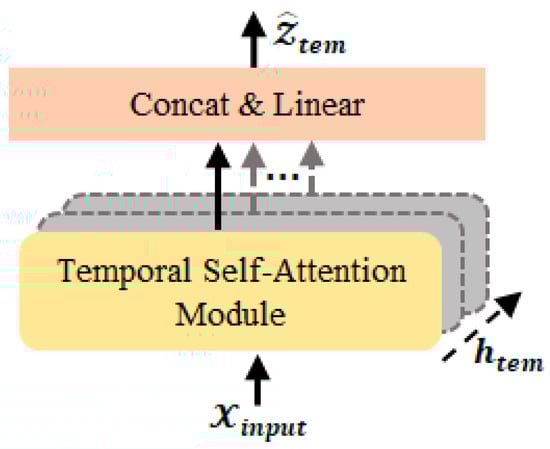
Figure 5.
The temporal self-attention module.
Here, is a learnable parameter matrix, and represents the positional encoding embedding vector of the current time step in the historical time steps. The positional encoding in this case adopts the same encoding method as the Transformer model [53].
Assuming the embedding matrix of an arbitrary node in the traffic network is denoted as , the calculation of the temporal self-attention is as follows:
where denote the Query, Key, and Value matrices, respectively, within the temporal self-attention mechanism. denotes the attention score. And are parameter matrices that can be learned, where represents the dimension of the Query, Key, and Value matrices within the temporal self-attention module. is the activation function.
Similarly to the computation process of spatial self-attention, this method can further obtain the final output of the temporal self-attention module:
where represents the number of heads in the temporal self-attention module, and is the upper bound of the number of heads for the temporal self-attention module. is a learnable parameter matrix.
In summary, the final output of the spatial–temporal attention layer is calculated as follows:
where is the layer normalisation operation, represents the concatenation operation, and is the learnable parameter matrix.
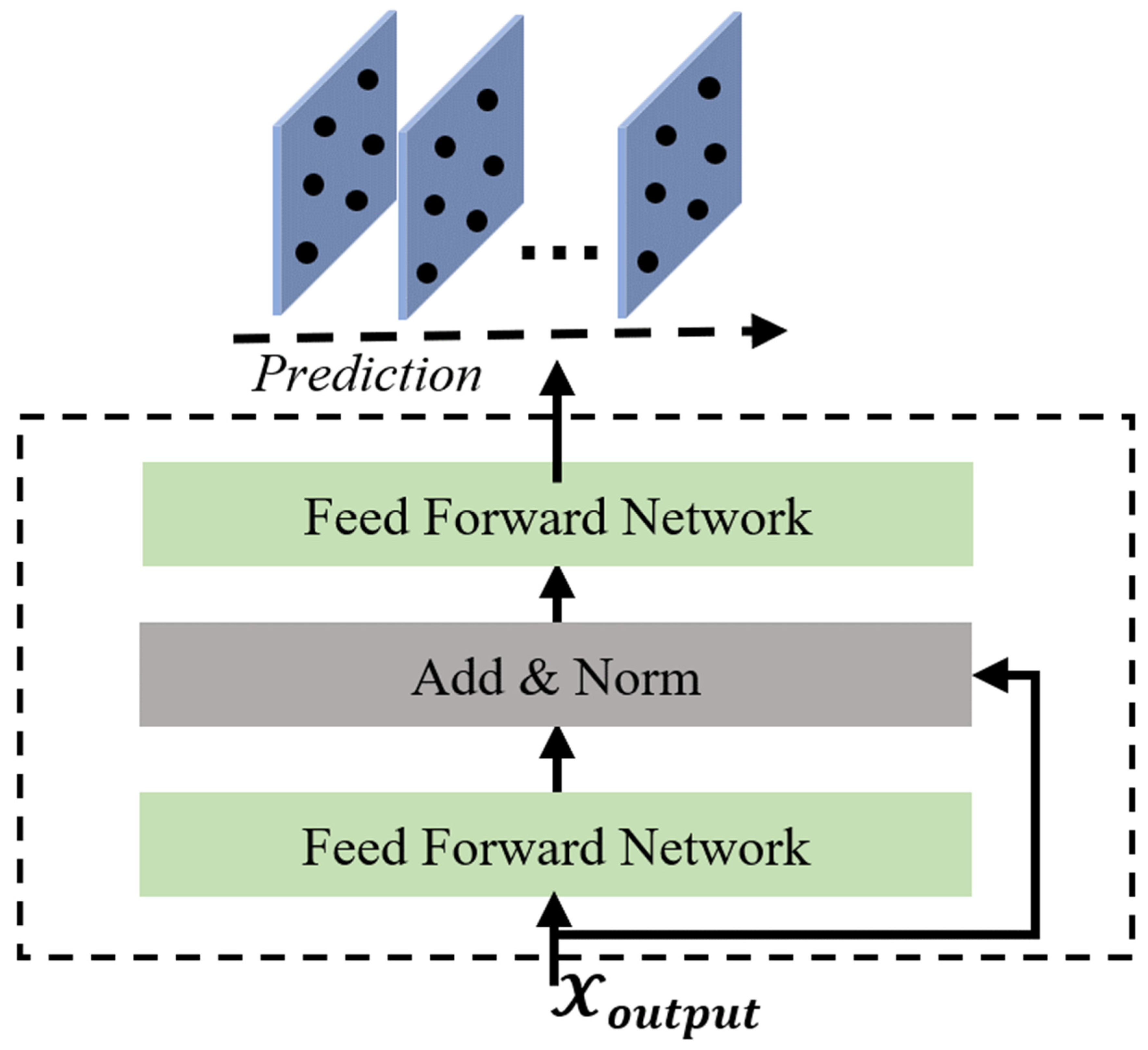
4.3. Output Layer
The output layer of the model comprises two feedforward neural networks, which are augmented with residual connections and layer normalisation operations (as illustrated in Figure 6). This design enables us to project the fused hidden representations, incorporating spatial–temporal dynamic dependencies, onto the final prediction space via the output layer:
where is the formal definition of the feedforward neural network. is the layer normalization operation and is the activation function.

Figure 6.
The output layer.
4.4. Model Training Strategy
This research utilises Huber loss [65] as the objective function. In contrast to the MAE and MSE loss functions, the Huber loss function combines the strengths of both while being less sensitive to outliers, thus exhibiting higher robustness. This makes it more suitable for predicting spatial–temporal sequence data. The Huber loss function is defined as follows:
where denotes the ground truth, denotes the predicted value for the th sample, and is a threshold used to control the smoothing range.
5. Experiments
5.1. Datasets
To validate the DSTSAN model, four real traffic datasets are selected and widely utilised in the PeMS system [66], namely PEMS03, PEMS04, PEMS07, and PEMS08. These datasets were collected by the Caltrans Performance Measurement System (PeMS) using sensors that span across major urban areas in the state of California, USA. The sensors collected data at a frequency of once every 30 s, and the collected data were aggregated every 5 min to form a data point. Each sensor accumulated 288 data points per day. The dataset includes information such as traffic speed, traffic flow, and the adjacency matrix of the traffic network. Table 1 presents a summary of the detailed parameters for the four datasets:

Table 1.
Statistics of datasets.
5.2. Baselines
To thoroughly validate the advantages of the DSTSAN model, this method performed comparative experiments with 11 representative baseline methods. These methods were selected based on their availability of the open-source code and are considered to be representative of the field. The selected baselines cover a range of approaches, including traditional time series prediction models, neural network-based models, Graph Neural Network-based models, and some of the more recent advanced methods.
- Vector Autoregression Model (VAR) [56]: The model first assumes a smooth historical time series state and then accomplishes the forecasting task by estimating the relationship between the time series and its lagged values;
- Autoregressive Integrated Moving Average Model (ARIMA) [19]: The model extracts the time series patterns hidden in the data by means of data autocorrelation and differencing, and then completes the prediction task through these patterns;
- Fully Connected Long Short-Term Memory Model (FC-LSTM) [67]: A Long Short-Term Memory network model with fully connected hidden units that can effectively capture dependencies in time series data;
- Diffusion Convolutional Recurrent Neural Network (DCRNN) [4]: The model integrates the features of bidirectional diffusion graph convolution and Recurrent Neural Networks to predict traffic flow accurately;
- Graph WaveNet [37]: The model adopts a hierarchical composition of Gate TCN (Temporal Convolutional Network) modules and GCN (Graph Convolutional Network) modules to model the spatial–temporal correlations in the traffic data effectively;
- Spatial–Temporal Graph Convolutional Networks (STGCNs) [2]: The model integrates Chebyshev graph convolution with 1D temporal convolution to effectively capture comprehensive spatial–temporal dependency features in the traffic data;
- Spatial–Temporal Fusion Graph Neural Networks (STFGNNs) [39]: The model leverages the fusion of spatial graphs and temporal graphs to capture hidden spatiotemporal dependencies in the traffic data effectively;
- Dynamic Spatial–Temporal Aware Graph Neural Networks (DSTAGNNs) [44]: The model incorporates dynamic spatial–temporal perception graph and improved gate convolutional modules to capture the inherent spatiotemporal dynamic features of the traffic data effectively;
- Graph Multi-Attention Network (GMAN) [29]: The multilevel attention model captures the dynamic spatiotemporal dependencies in the traffic data by stacking various attention modules, including spatial attention, temporal attention, and self-attention;
- Spatial–Temporal Graph Neural Controlled Differential Equations (STG-NCDEs) [59]: The temporal dynamics of the traffic data are modelled using the neural control differential equations, while leveraging the Graph Convolutional Networks to capture the spatial dependencies among different data points;
- Propagation Delay-aware Dynamic Long-range Transformer (PDFormer) [13]: The model utilises the self-attention mechanism to capture the dependencies in the traffic data. It introduces different graph mask matrices to model local spatial dependencies and global spatial dependencies separately. Additionally, the model incorporates a traffic delay perception feature module to address the issue of time delay in the spatial information propagation process.
5.3. Experimental Setups
The experiments were performed on a server that was equipped with two NVIDIA Tesla P100 GPUs, each having 16 GB of memory, and had a storage capacity of 256 GB. The server was running on the Ubuntu 20.04 operating system. The DSTSAN model was implemented using Pytorch 1.13.0 and Python 3.10.6.
To ensure the validity of the comparative experiments, this research adhered to the experimental settings commonly used in most baseline methods. The four datasets were divided into training, validation, and testing sets in a proportion of 6:2:2, respectively. For the prediction task, we utilised 12 historical time steps to forecast the subsequent 12 time steps of traffic flow conditions, denoted as . As this research only considered traffic data from the datasets, the traffic signal dimension, D, was set to 1. The model was trained using the AdamW optimiser [13], with a learning rate of 0.001. The batch size for the data was set to 32, and the training process was conducted for 200 epochs. Additionally, the early stopping strategy was applied to the validation set with a patience value of 15.
The performance of model has been assessed using three metrics: Mean Absolute Error (MAE), Mean Absolute Percentage Error (MAPE), and Root Mean Squared Error (RMSE). The MAE measures the absolute difference between the predicted values and the actual values, providing an indication of the accuracy of the predictions. The RMSE quantifies the difference between the predicted value and the ground truth, primarily serving as a measure of how well the model fits the data, as well as being sensitive to outliers. The MAPE represents the percentage error between the predicted results and the actual observed values, providing insights into the relative degree of error between the predictions and the ground truth. The formulas for these metrics are as follows:
where denotes the th ground truth, represents the th predicted value, and represents the number of samples, which in this experiment is set to 12. Moreover, this research performed data pre-processing by removing instances with missing values and filtering out data samples with a traffic volume below 10 to mitigate the impact of noise. To ensure robustness, all experiments are repeated 10 times and calculated the average values as the final results.
5.4. Experiment Results
The experimental results comparing DSTSAN with other baseline methods on four real datasets are presented in Table 2. The best results are highlighted in bold. Based on the analysis of Table 2, the following conclusions can be drawn:
Table 2.
Performance comparison of DSTSAN and others baseline models.
- (1)
- Methods incorporating neural networks, Graph Neural Networks, and attention mechanisms generally outperform traditional time series forecasting models such as VAR and ARIMA. This is attributed to the fact that traditional time series forecasting models often rely on static assumptions, which are insufficient for capturing the highly nonlinear spatial dependencies present in the traffic data. Consequently, these traditional models tend to overlook crucial information, resulting in an unsatisfactory prediction performance;
- (2)
- Graph Neural Network models, such as STGNN and Graph WaveNet, exhibit substantial advantages over neural network models like FC-LSTM and DCRNN in terms of prediction performance. This is attributed to the ability of Graph Neural Network models to effectively model both local and global spatial dependencies present in the traffic data, enabling them to capture a richer set of essential information compared to the aforementioned models. Furthermore, attention-based methods outperform Graph Neural Network-based methods. This can be attributed to the superior capability of attention mechanisms in integrating dynamic spatiotemporal dependencies present in the traffic data;
- (3)
- It is not universally true that methods based on Graph Neural Networks or attention mechanisms are always superior to other approaches. For instance, the STG-NCDE model, which combines neural controlled differential equations with Graph Convolutional Network models, exhibits comparable performance and competitiveness. This suggests that there is diversity in the solutions for the same problem, and different approaches can yield competitive results;
- (4)
- This model demonstrates a superior performance compared to other baseline methods for several reasons. Firstly, a comprehensive consideration of both local and global spatial dependencies is incorporated in the spatial dimension. Additionally, in the temporal dimension, this method accounts for the multi-periodicity of traffic flow. This holistic approach to spatial and temporal factors contributes to the improved performance of this model. Secondly, a feature augmentation layer is introduced that automatically adjusts the information interaction among different features. This feature augmentation facilitates the enhancement of representation capabilities for each feature dimension, resulting in an improved overall performance. Lastly, this model utilises two spatiotemporal attention modules to effectively capture and integrate the dynamic spatiotemporal dependencies present in the traffic data. This enables the model to accurately capture the complex patterns and relationships within the data, leading to more precise predictions.
5.5. Ablation Study
To further investigate the effectiveness of each core module in the DSTSAN model, modifications were made to the core modules, and comparative experiments were conducted between the modified variants and the original DSTSAN model. Specifically, this research performed the following variant experiments:
- (1)
- Variant FA: removal of the feature enhancement layer;
- (2)
- Variant Mh: spatial self-attention module using only the mask matrix, considering only local spatial dependencies;
- (3)
- Variant Ms: spatial self-attention module using only the mask matrix, considering only global spatial dependencies;
- (4)
- Variant TSA: removal of the temporal self-attention module.
By comparing these variant models with the original DSTSAN model, this method can assess the performance differences and evaluate the contributions of each core module to the model’s performance.
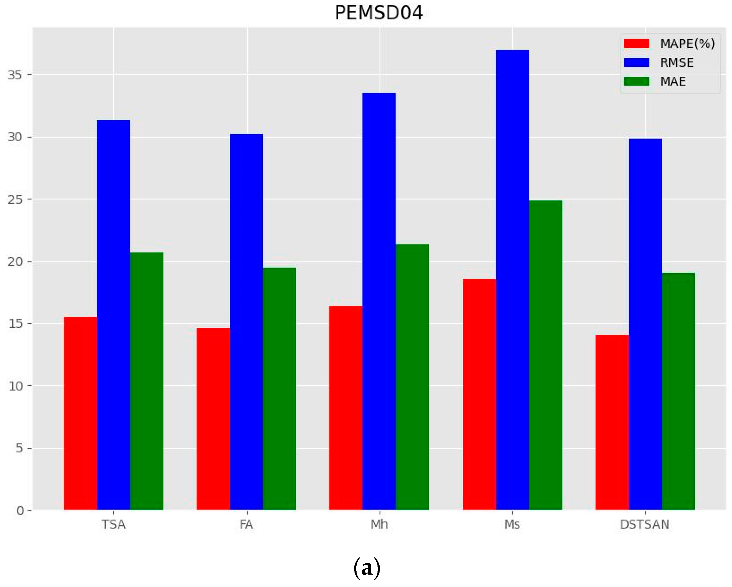
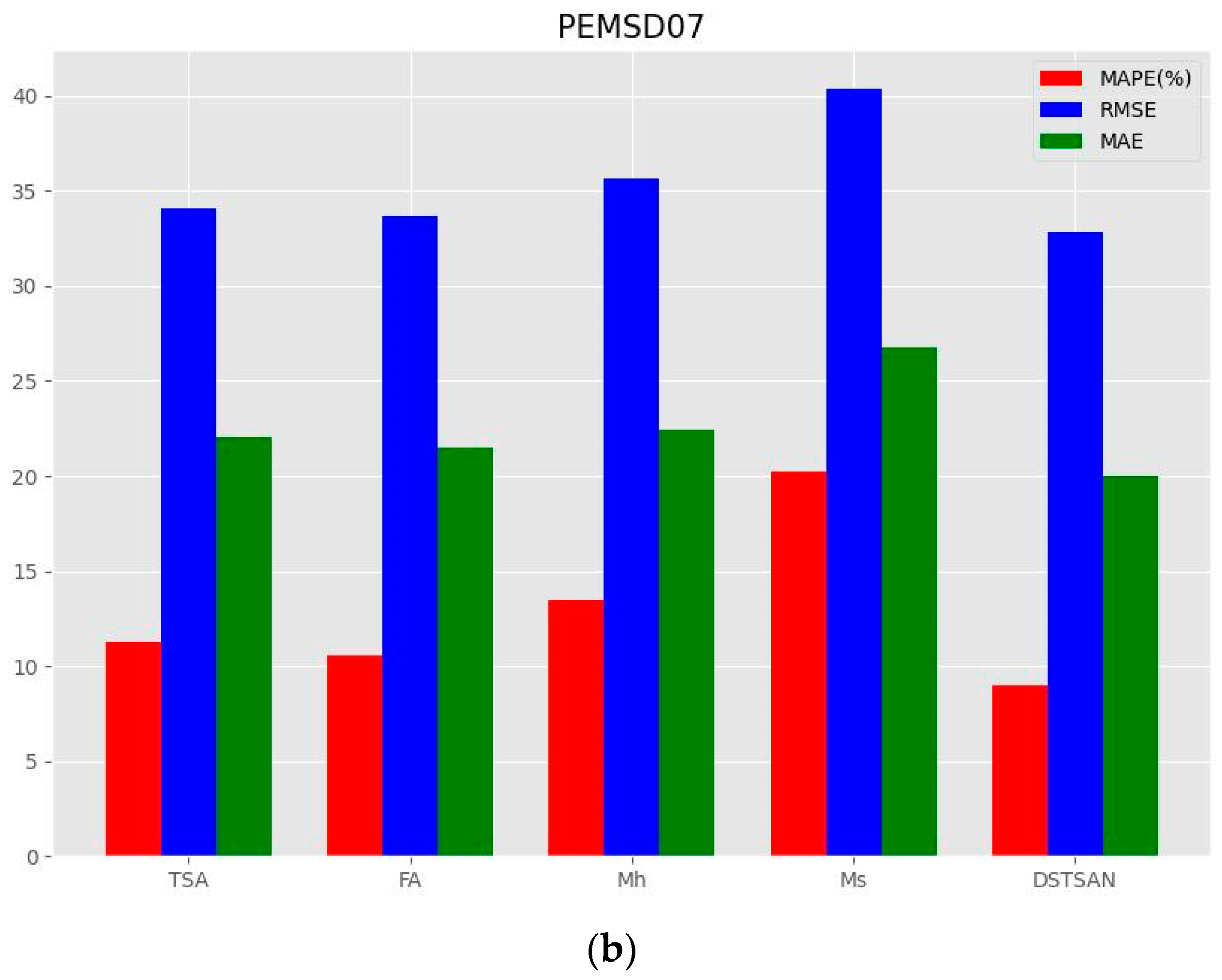
This experiment conducted comparative experiments between DSTSAN and its variants on the PEMS04 and PEMS07 datasets, as shown in Figure 7:

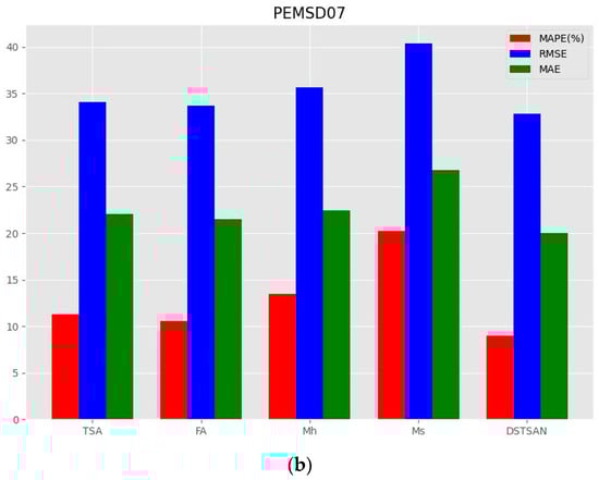
Figure 7.
Ablation studies. (a) Ablation study on PEMS04. (b) Ablation study on PEMS07.
- (1)
- The absence of any core module in the DSTSAN leads to a decrease in the model’s predictive performance, indicating that all core modules in the model capture key information to some extent;
- (2)
- The model exhibits the most significant decrease in predictive performance when only considering global spatial dependencies, indicating that local spatial dependencies have the greatest impact on the model’s predictive performance. Furthermore, this suggests that the traffic conditions at a road node are most influenced by the traffic conditions at its adjacent road nodes, aligning with the real-life observations;
- (3)
- In addition to local spatial correlations, global spatial correlations and dynamic temporal correlations are also crucial for influencing traffic flow.
5.6. Parameter Sensitivity Studies
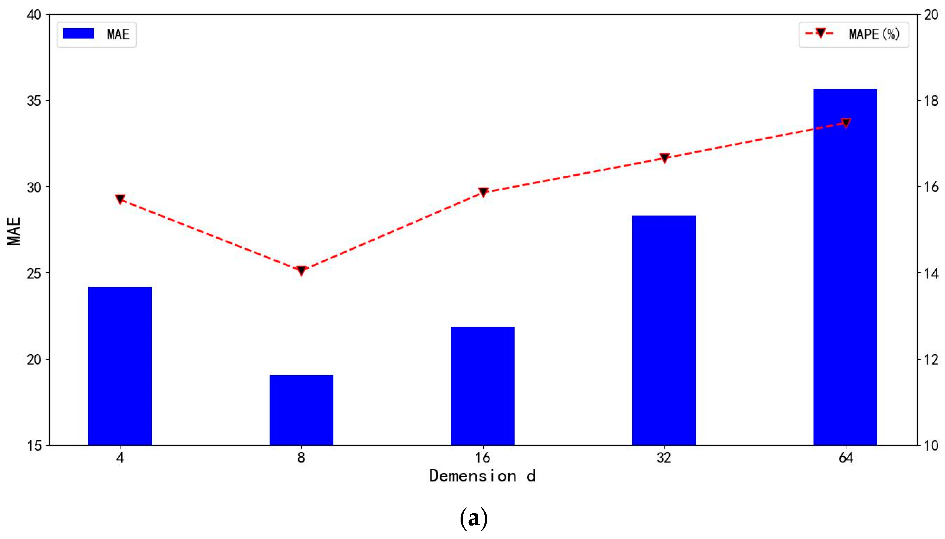
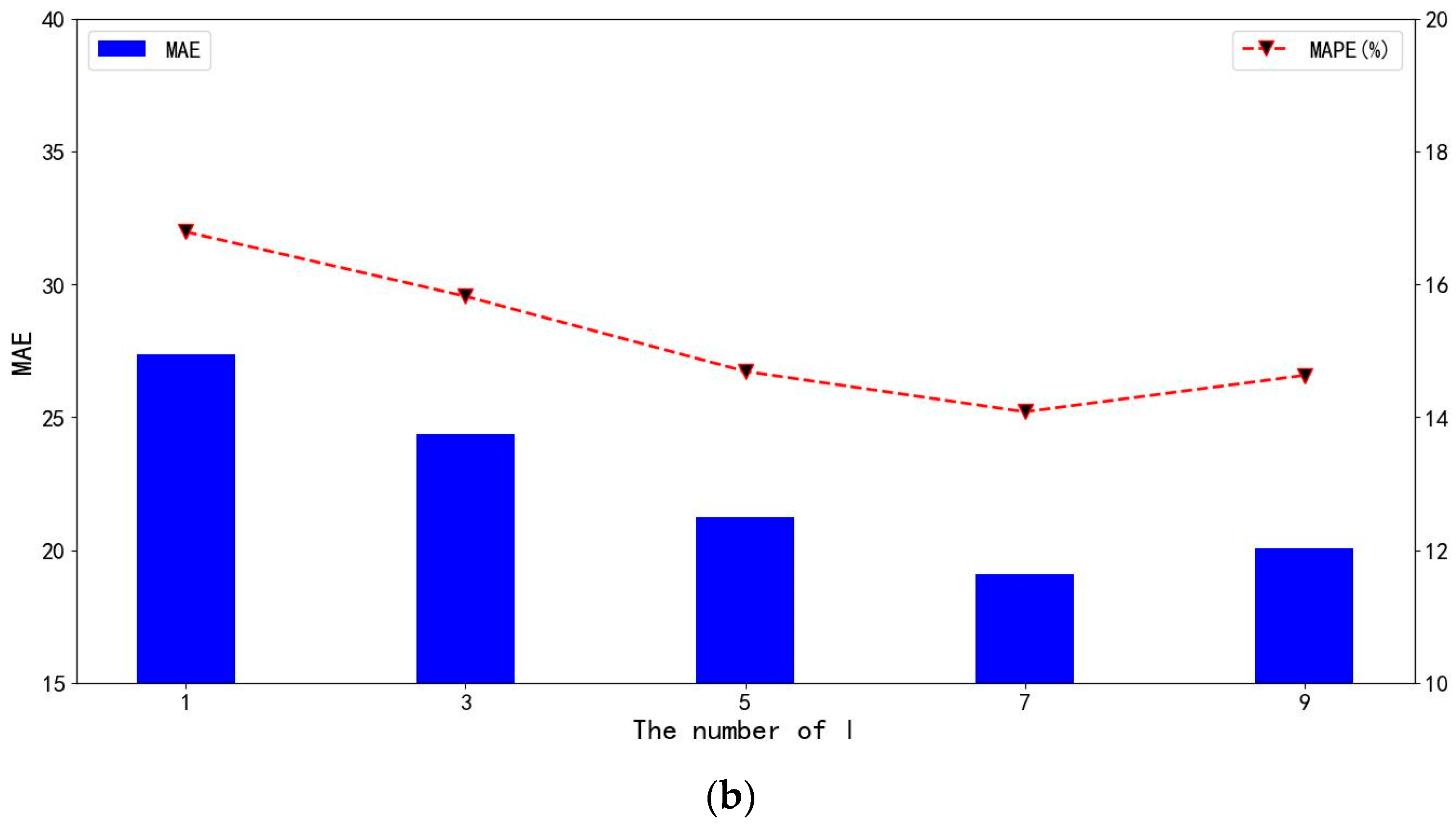
To investigate the impact of certain parameter settings in the model on traffic flow prediction results, parameter sensitivity tests were conducted on the data embedding dimension and the number of layers for spatiotemporal self-attention on the PEMS04 dataset. For the data embedding dimension , this research tested values of , and the results are shown in Figure 8a in terms of MAE and MAPE. For the number of layers for spatiotemporal self-attention , this method tested values of , and the results are shown in Figure 8b in terms of MAE and MAPE.


Figure 8.
The effects of the parameters. (a) The effects of the embedding dimension . (b) The effects of spatial–temporal self-attention layer .
Figure 8a demonstrates that the predictive performance of the model follows a trend of initially increasing and then decreasing as the embedding dimension increases, reaching its optimum at . This is because as the embedding dimension increases from small to large, the embedded information increases, enhancing the expressive power of the model and enabling it to capture more crucial information. However, as the embedding dimension continues to increase, the number of parameters also increases, which may lead to model overfitting and consequently result in a decline in performance. This indicates that in selecting the embedding dimension, it is necessary to balance the model’s expressive power and the risk of overfitting, thereby choosing an appropriate embedding dimension to achieve optimal predictive performance.
From Figure 8b, it can be observed that the predictive performance of the model exhibits an increasing and then decreasing trend as the number of self-attention layers increases. The model achieves its optimal predictive performance when the number of layers is , and subsequent increases in the number of layers lead to a decline in the model’s predictive capability. This is because in the initial stage, as the number of layers increases, the model captures an increasing amount of key information. However, when the number of layers exceeds a certain threshold, the model starts to overfit, leading to a decrease in the accuracy of the predictions.
In summary, the model DSTSAN is sensitive to the data embedding dimension and the number of self-attention layers .
6. Conclusions
This paper proposes a new Dynamic Spatial–Temporal Self-Attention Network model (DSTSAN) to solve the traffic flow prediction problem. Compared to current approaches that focus only on local dependencies in traffic flow data based on the topology of traffic networks, this approach, based on the spatial self-attention module, achieves effective modelling of local spatial correlations and global spatial correlations in traffic flow data through the introduction of spatial masking matrices and semantic masking matrices. As for some current approaches that focus only on spatial dependencies, this approach not only models the features such as daily periodicity and weekly periodicity that traffic flow exhibits in real life, but it also fuses the dynamic temporal dependencies in traffic flow data through the temporal self-attention module. The effectiveness of the proposed method is verified through comparison tests with 11 representative baseline methods on four real traffic flow datasets.
However, there are some limitations in this approach: (1) There are many conditions that affect the traffic flow conditions, such as weather, temporary activities, etc., for which the approach has not been able to model such features effectively. (2) The computational cost in this model is high due to the computation of multiple multi-head self-attention mechanisms, and the model is inefficiently executed when the amount of data is large. As a result, subsequent work will also focus on addressing the issues of improving model performance and execution efficiency, as well as multimodal feature fusion for traffic flow.
Author Contributions
Conceptualization, H.Z.; Methodology, H.Y.; Software, D.W. and H.Z.; Validation, D.W. and H.Z.; Formal Analysis, H.Y. and H.Z.; Writing, D.W.; Review and Editing, H.Y. and H.Z. All authors have read and agreed to the published version of the manuscript.
Funding
This research was partially supported by the project “Research on Key Common Technology of Digital Industry Innovation Platform”: 01108/110822150.
Data Availability Statement
All datasets in this paper are publicly available datasets.
Conflicts of Interest
The authors declare no conflicts of interest.
References
- Wootton, J.R.; Garcia-Ortiz, A.; Amin, S.M. Intelligent Transportation Systems: A Global Perspective. Math. Comput. Model. 1995, 22, 4–7. [Google Scholar] [CrossRef]
- Yu, B.; Yin, H.; Zhu, Z. Spatio-Temporal Graph Convolutional Networks: A Deep Learning Framework for Traffic Forecasting. In Proceedings of the 27th International Joint Conference on Artificial Intelligence (IJCAI), Stockholm, Sweden, 13–19 July 2018. [Google Scholar] [CrossRef]
- Wei, H.; Zheng, G.; Yao, H.; Li, Z.J. IntelliLight: A Reinforcement Learning Approach for Intelligent Traffic Light Control. In Proceedings of the 24th ACM SIGKDD International Conference on Knowledge Discovery & Data Mining, London, UK, 19–23 August 2018. [Google Scholar]
- Li, Y.; Yu, R.; Shahabi, C.; Liu, Y. Diffusion Convolutional Recurrent Neural Network: Data-Driven Traffic Forecasting. arXiv 2017, arXiv:1707.01926. [Google Scholar] [CrossRef]
- Huang, C.; Zhang, C.; Dai, P.; Bo, L. Cross-Interaction Hierarchical Attention Networks for Urban Anomaly Prediction. In Proceedings of the Twenty-Ninth International Conference on International Joint Conferences on Artificial Intelligence, Online, 7–15 January 2021. [Google Scholar]
- Tedjopurnomo, D.A.; Bao, Z.; Zheng, B.; Choudhury, F.M.; Qin, A.K. A Survey on Modern Deep Neural Network for Traffic Prediction: Trends, Methods, and Challenges. IEEE Trans. Knowl. Data Eng. 2020, 34, 1544–1561. [Google Scholar] [CrossRef]
- Wu, Y.; Tan, H. Short-term Traffic Flow Forecasting with Spatial-temporal Correlation in a Hybrid Deep Learning Framework. arXiv 2016, arXiv:1612.01022. [Google Scholar] [CrossRef]
- Medina-Salgado, B.; Sánchez-DelaCruz, E.; Pozos-Parra, P.; Sierra, J.E. Urban Traffic Flow Prediction Techniques: A Review. Sustain. Comput. Inform. Syst. 2022, 35, 100739. [Google Scholar] [CrossRef]
- He, S.; Shin, K.G. Towards Fine-grained Flow Forecasting: A Graph Attention Approach for Bike Sharing Systems. In Proceedings of the Web Conference 2020, Taipei, Taiwan, 20–24 April 2020. [Google Scholar]
- Rao, X.; Wang, H.; Zhang, L.; Li, J.; Shang, S.; Han, P. FOGS: First-Order Gradient Supervision with Learning-based Graph for Traffic Flow Forecasting. In Proceedings of the Thirty-First International Joint Conference on Artificial Intelligence (IJCAI-22), Vienna, Austria, 23–29 July 2022. [Google Scholar]
- Shao, Z.; Zhang, Z.; Wei, W.; Wang, F.; Xu, Y.; Cao, X.; Jensen, C.S. Decoupled Dynamic Spatial-Temporal Graph Neural Network for Traffic Forecasting. Proc. VLDB Endow. 2022, 15, 2733–2746. [Google Scholar] [CrossRef]
- Lee, H.; Park, C.; Jin, S.; Chu, H.; Choo, J.; Ko, S. An Empirical Experiment on Deep Learning Models for Predicting Traffic Data. In Proceedings of the 2021 IEEE 37th International Conference on Data Engineering (ICDE), Chania, Greece, 19–22 April 2021; pp. 1817–1822. [Google Scholar]
- Jiang, J.; Han, C.; Zhao, W.X.; Wang, J. PDFormer: Propagation Delay-aware Dynamic Long-range Transformer for Traffic Flow Prediction. In Proceedings of the AAAI Conference on Artificial Intelligence, Washington, DC, USA, 7–14 February 2023. [Google Scholar]
- Wu, J.; Fu, J.C.; Ji, H.; Liu, L. Graph Convolutional Dynamic Recurrent Network with Attention for Traffic Forecasting. Appl. Intell. 2023, 53, 22002–22016. [Google Scholar] [CrossRef]
- Navarro-Espinoza, A.; López-Bonilla, O.R.; García-Guerrero, E.E.; Tlelo-Cuautle, E.; López-Mancilla, D.; Hernández-Mejía, C.; Inzunza-González, E. Traffic Flow Prediction for Smart Traffic Lights Using Machine Learning Algorithms. Technologies 2022, 10, 5. [Google Scholar] [CrossRef]
- Singh, A.; Yadav, A.; Rana, A.K. K-means with Three Different Distance Metrics. Int. J. Comput. Appl. 2013, 67, 10. [Google Scholar] [CrossRef]
- Cascetta, E. Transportation Systems Engineering: Theory and Methods; Springer: Berlin/Heidelberg, Germany, 2001. [Google Scholar]
- Li, F.; Feng, J.; Yan, H.; Jin, G.; Jin, D.; Li, Y. Dynamic Graph Convolutional Recurrent Network for Traffic Prediction: Benchmark and Solution. ACM Trans. Knowl. Discov. Data 2021, 17, 1–21. [Google Scholar] [CrossRef]
- Kumar, S.V.; Vanajakshi, L.D. Short-term Traffic Flow Prediction Using Seasonal ARIMA Model with Limited Input Data. Eur. Transport Res. Rev. 2015, 7, 1–9. [Google Scholar] [CrossRef]
- Cho, K.; Merrienboer, B.V.; Bahdanau, D.; Bengio, Y. On the Properties of Neural Machine Translation: Encoder–Decoder Approaches. arXiv 2014, arXiv:1409.1259. [Google Scholar]
- Wu, C.-H.; Ho, J.-M.; Lee, D.T. Travel-time Prediction with Support Vector Regression. IEEE Trans. Intell. Transp. Syst. 2004, 5, 276–281. [Google Scholar] [CrossRef]
- Dong, X.; Lei, T.; Jin, S.; Hou, Z. Short-Term Traffic Flow Prediction Based on XGBoost. In Proceedings of the 2018 IEEE 7th Data Driven Control and Learning Systems Conference (DDCLS), Enshi, China, 25–27 May 2018; pp. 854–859. [Google Scholar]
- Bai, L.; Yao, L.; Kanhere, S.S.; Yang, Z.; Chu, J.; Wang, X. Passenger Demand Forecasting with Multi-Task Convolutional Recurrent Neural Networks. In Proceedings of the Pacific-Asia Conference on Knowledge Discovery and Data Mining, Macau, China, 14–17 April 2019. [Google Scholar]
- Bai, L.; Yao, L.; Li, C.; Wang, X.; Wang, C. Adaptive Graph Convolutional Recurrent Network for Traffic Forecasting. In Proceedings of the 34th Conference on Neural Information Processing Systems (NeurIPS 2020), Online, 6–12 December 2020; Curran Associates Inc.: Red Hook, NY, USA, 2020. Article 1494. pp. 17804–17815. [Google Scholar]
- Chen, Y.; Segovia, I.; Gel, Y.R. Z-GCNETs: Time Zigzags at Graph Convolutional Networks for Time Series Forecasting. In Proceedings of the International Conference on Machine Learning, Online, 18–24 July 2021; pp. 1684–1694. [Google Scholar]
- Hochreiter, S.; Schmidhuber, J. Long Short-Term Memory. Neural Comput. 1997, 9, 1735–1780. [Google Scholar] [CrossRef] [PubMed]
- Chung, J.; Gulcehre, C.; Cho, K.; Bengio, Y. Empirical Evaluation of Gated Recurrent Neural Networks on Sequence Modeling. In NIPS 2014 Workshop on Deep Learning; Elsevier: Amsterdam, The Netherlands, 2014. [Google Scholar]
- Guo, S.; Lin, Y.; Feng, N.; Song, C.; Wan, H. Attention Based Spatial-Temporal Graph Convolutional Networks for Traffic Flow Forecasting. Proc. AAAI Conf. Artif. Intell. 2019, 33, 922–929. [Google Scholar] [CrossRef]
- Zheng, C.; Fan, X.; Wang, C.; Qi, J. GMAN: A Graph Multi-Attention Network for Traffic Prediction. Proc. AAAI Conf. Artif. Intell. 2020, 34, 1234–1241. [Google Scholar] [CrossRef]
- Wu, Z.; Pan, S.; Long, G.; Jiang, J.; Chang, X.; Zhang, C. Connecting the Dots: Multivariate Time Series Forecasting with Graph Neural Networks. In Proceedings of the 26th ACM SIGKDD International Conference on Knowledge Discovery & Data Mining, Virtual Event, 23–27 August 2020. [Google Scholar]
- Zhang, Q.; Chang, J.; Meng, G.; Xiang, S.; Pan, C. Spatio-Temporal Graph Structure Learning for Traffic Forecasting. Proc. AAAI Conf. Artif. Intell. 2020, 34, 1177–1185. [Google Scholar] [CrossRef]
- Huang, R.; Huang, C.; Liu, Y.; Dai, G.; Kong, W. LSGCN: Long Short-Term Traffic Prediction with Graph Convolutional Networks. In Proceedings of the Twenty-Ninth International Joint Conference on Artificial Intelligence (IJCAI-20), Yokohama, Japan, 7–15 January 2021. [Google Scholar]
- Pinaya, W.H.L.; Vieira, S.; Garcia-dias, R.; Mechelli, A. Convolutional Neural Networks; Machine learning; Academic Press: Cambridge, MA, USA, 2020; pp. 173–191. [Google Scholar]
- Scarselli, F.; Gori, M.; Tsoi, A.C.; Hagenbuchner, M.; Monfardini, G. The Graph Neural Network Model. IEEE Trans. Neural Netw. 2009, 20, 61–80. [Google Scholar] [CrossRef] [PubMed]
- Zhou, J.; Cui, G.; Hu, S.; Zhang, Z.; Yang, C.; Liu, Z.; Wang, L.; Li, C.; Sun, M. Graph Neural Networks: A Review of Methods and Applications. AI Open 2020, 1, 57–81. [Google Scholar] [CrossRef]
- Wu, Z.; Pan, S.; Chen, F.; Long, G.; Zhang, C.; Yu, P.S. A Comprehensive Survey on Graph Neural Networks. IEEE Trans. Neural Netw. Learn. Syst. 2019, 32, 4–24. [Google Scholar] [CrossRef]
- Wu, Z.; Pan, S.; Long, G.; Jiang, J.; Zhang, C. Graph WaveNet for Deep Spatial-Temporal Graph Modeling. In Proceedings of the Twenty-Eighth International Joint Conference on Artificial Intelligence (IJCAI-19), Macao, China, 10–16 August 2019. [Google Scholar]
- Rahmani, S.; Baghbani, A.; Bouguila, N.; Patterson, Z. Graph Neural Networks for Intelligent Transportation Systems: A Survey. IEEE Trans. Intell. Transp. Syst. 2023, 24, 8846–8885. [Google Scholar] [CrossRef]
- Li, M.; Zhu, Z. Spatial-temporal Fusion Graph Neural Networks for Traffic Flow Forecasting. Proc. AAAI Conf. Artif. Intell. 2021, 35, 4189–4196. [Google Scholar] [CrossRef]
- Seo, Y.; Defferrard, M.; Vandergheynst, P.; Bresson, X. Structured Sequence Modeling with Graph Convolutional Recurrent Networks. In Neural Information Processing: Proceedings of the 25th International Conference, ICONIP 2018, Siem Reap, Cambodia, 13–16 December 2018; Proceedings, Part I; Springer International Publishing: Berlin/Heidelberg, Germany, 2018; pp. 362–373. [Google Scholar]
- Yan, S.; Xiong, Y.; Lin, D. Spatial Temporal Graph Convolutional Networks for Skeleton-Based Action Recognition. Proc. AAAI Conf. Artif. Intell. 2018, 32, 1. [Google Scholar] [CrossRef]
- Kipf, T.N.; Welling, M. Semi-Supervised Classification with Graph Convolutional Networks. arXiv 2016, arXiv:1609.02907. [Google Scholar] [CrossRef]
- Defferrard, M.; Bresson, X.; Vandergheynst, P. Convolutional Neural Networks on Graphs with Fast Localized Spectral Filtering. In Proceedings of the 30th Conference on Neural Information Processing Systems (NIPS 2016), Barcelona, Spain, 5–10 December 2016. [Google Scholar]
- Lan, S.; Ma, Y.; Huang, W.; Wang, W.; Yang, H.; Li, P. DSTAGNN: Dynamic Spatial-Temporal Aware Graph Neural Network for Traffic Flow Forecasting. In Proceedings of the 39th International Conference on Machine Learning, Baltimore, MD, USA, 17–23 July 2022. [Google Scholar]
- Liu, H.; Zhu, C.; Zhang, D.; Li, Q. Attention-based Spatial-Temporal Graph Convolutional Recurrent Networks for Traffic Forecasting. In Proceedings of the International Conference Advanced Data Mining and Applications, Shenyang, China, 21–23 August 2023. [Google Scholar]
- Bruna, J.; Zaremba, W.; Szlam, A.; LeCun, Y. Spectral Networks and Locally Connected Networks on Graphs. arXiv 2013, arXiv:1312.6203. [Google Scholar]
- Micheli, A. Neural Network for Graphs: A Contextual Constructive Approach. IEEE Trans. Neural Netw. 2009, 20, 498–511. [Google Scholar] [CrossRef] [PubMed]
- Jiang, W.; Luo, J. Graph Neural Network for Traffic Forecasting: A Survey. Expert Syst. Appl. 2022, 207, 117921. [Google Scholar] [CrossRef]
- Gilmer, J.; Schoenholz, S.S.; Riley, P.F.; Vinyals, O.; Dahl, G.E. Neural Message Passing for Quantum Chemistry. In Proceedings of the 34th International Conference on Machine Learning, Sydney, Australia, 6–11 August 2017. [Google Scholar]
- Hamilton, W.L.; Ying, Z.; Leskovec, J. Inductive Representation Learning on Large Graphs. In Proceedings of the Thirty-first Annual Conference on Neural Information Processing Systems (NIPS), Long Beach, CA, USA, 4–9 December 2017. [Google Scholar]
- Atwood, J.; Towsley, D.F. Diffusion-Convolutional Neural Networks. In Proceedings of the Annual Conference on Neural Information Processing Systems 2015, Montreal, QC, Canada, 7–12 December 2015. [Google Scholar]
- Velickovic, P.; Cucurull, G.; Casanova, A.; Romero, A.; Liò, P.; Bengio, Y. Graph Attention Networks. Stat 2017, 1050, 10–48550. [Google Scholar]
- Vaswani, A.; Shazeer, N.M.; Parmar, N.; Uszkoreit, J.; Jones, L.; Gomez, A.N.; Kaiser, L.; Polosukhin, I. Attention is All You Need. In Proceedings of the Thirty-first Annual Conference on Neural Information Processing Systems (NIPS), Long Beach, CA, USA, 4–9 December 2017. [Google Scholar]
- Zhou, H.; Zhang, S.; Peng, J.; Zhang, S.; Li, J.; Xiong, H.; Zhang, W. Informer: Beyond Efficient Transformer for Long Sequence Time-Series Forecasting. Proc. AAAI Conf. Artif. Intell. 2021, 35, 11106–11115. [Google Scholar] [CrossRef]
- Lai, G.; Chang, W.-C.; Yang, Y.; Liu, H. Modeling Long- and Short-Term Temporal Patterns with Deep Neural Networks. In Proceedings of the 41st International ACM SIGIR Conference on Research & Development in Information Retrieval, Ann Arbor, MI, USA, 8–12 July 2017. [Google Scholar]
- Zivot, E.; Wang, J. Vector Autoregressive Models for Multivariate Time Series. 2003. Available online: https://faculty.washington.edu/ezivot/econ584/notes/varModels.pdf (accessed on 21 April 2024).
- Williams, B.M.; Hoel, L.A. Modeling and Forecasting Vehicular Traffic Flow as a Seasonal ARIMA Process: Theoretical Basis and Empirical Results. J. Transp. Eng. 2003, 129, 664–672. [Google Scholar] [CrossRef]
- Huang, S.; Wang, D.; Wu, X.; Tang, A. DSANet: Dual Self-Attention Network for Multivariate Time Series Forecasting. In Proceedings of the 28th ACM International Conference on Information and Knowledge Management, Beijing China, 3–7 November 2019. [Google Scholar]
- Choi, J.; Choi, H.; Hwang, J.; Park, N. Graph Neural Controlled Differential Equations for Traffic Forecasting. Proc. AAAI Conf. Artif. Intell. 2022, 36, 6367–6374. [Google Scholar] [CrossRef]
- Fang, Z.; Long, Q.; Song, G.; Xie, K. Spatial-Temporal Graph ODE Networks for Traffic Flow Forecasting. In Proceedings of the 27th ACM SIGKDD Conference on Knowledge Discovery and Data Mining, Virtual Event, 14–18 August 2021. [Google Scholar]
- Jin, G.; Liu, L.; Li, F.; Huang, J. Spatio-Temporal Graph Neural Point Process for Traffic Congestion Event Prediction. Proc. AAAI Conf. Artif. Intell. 2023, 37, 14268–14276. [Google Scholar] [CrossRef]
- Berndt, D.J.; Clifford, J. Using Dynamic Time Warping to Find Patterns in Time Series. In Proceedings of the KDD Workshop, Seattle, WA, USA, 31 July–1 August 1994. [Google Scholar]
- Woo, S.; Park, J.; Lee, J.Y.; Kweon, I.S. CBAM: Convolutional Block Attention Module. In Proceedings of the 15th European Conference on Computer Vision, Munich, Germany, 8–14 September 2018; pp. 3–19. [Google Scholar]
- Keogh, E.J.; Pazzani, M.J. Derivative Dynamic Time Warping. In Proceedings of the 2001 SIAM International Conference on Data Mining, Chicago, IL, USA, 5–7 April 2001. [Google Scholar]
- Huber, P.J. Robust Estimation of a Location Parameter. Ann. Math. Stat. 1964, 35, 492–518. [Google Scholar] [CrossRef]
- Chen, C.; Petty, K.; Skabardonis, A.; Varaiya, P.; Jia, Z. Freeway performance measurement system: Mining loop detector data. Transp. Res. Rec. 2001, 1748, 96–102. [Google Scholar] [CrossRef]
- Sutskever, I.; Vinyals, O.; Le, Q.V. Sequence to Sequence Learning with Neural Networks. Adv. Neural Inf. Process. Syst. 2014, 27, 3104. Available online: https://proceedings.neurips.cc/paper_files/paper/2014/hash/a14ac55a4f27472c5d894ec1c3c743d2-Abstract.html (accessed on 21 May 2024).

Disclaimer/Publisher’s Note: The statements, opinions and data contained in all publications are solely those of the individual author(s) and contributor(s) and not of MDPI and/or the editor(s). MDPI and/or the editor(s) disclaim responsibility for any injury to people or property resulting from any ideas, methods, instructions or products referred to in the content. |
© 2024 by the authors. Licensee MDPI, Basel, Switzerland. This article is an open access article distributed under the terms and conditions of the Creative Commons Attribution (CC BY) license (https://creativecommons.org/licenses/by/4.0/).