Methodology to Improve an Extended-Range Electric Vehicle Module and Control Integration Based on Equivalent Consumption Minimization Strategy

Abstract

The continuous expansion of the vehicle fleet contributes to escalating emissions, with the transportation sector accounting for approximately 21% of CO₂ emissions, based on 2023 data. Focused on reducing emissions and reliance on fossil fuels, the study observes the shift from internal combustion vehicles to electric and hybrid models since 2017. Despite advancements, these vehicles still lack optimal efficiency and suffer from limited range, deterring potential buyers. This article aims to evaluate the range-extending technologies for electric vehicles, emphasizing efficiency, low pollution, and integration compatibility. An algorithm incorporating equations representing mechanical or electrical component curves is developed for Extended-Range Electric Vehicles, facilitating insight into potential range extender behavior. The core objectives of this study involve optimizing the entire powertrain system to ensure peak efficiency. Experimental tests demonstrate that integrating an auxiliary power unit enhances range, with an internal combustion engine generator configuration extending the travel distance by 35.35% at a constant speed. Moreover, with the use of an Equivalent Consumption Minimization Strategy control, the distance traveled increases up to 39.28% on standard driving cycles. The proposed methodology, validated through practical implementations, allows for comprehensive energy analyses, providing a precise understanding of vehicle platform performance with integrated range extenders.

1. Introduction

The growing global automotive fleet has led to an increase in carbon emissions released into the environment, with the transportation sector contributing approximately 21% of CO₂ emissions [1]. Addressing this issue requires the development of vehicles with new technologies and the advancement of clean energy for their use, moving away from the dependence on fossil fuels. Consequently, sales of internal combustion engine vehicles peaked in 2017 [2], and since then, sales of electric and hybrid vehicles have been growing annually. However, despite their lower environmental impact, they have not yet achieved widespread adoption, as the limited range of electric vehicles continues to detract from their appeal to potential buyers.

To overcome these challenges, significant research efforts have focused on improving vehicle drivetrains. In this regard, extending the range of electric vehicles has been a topic of debate, and the potential of auxiliary power units (APUs) as a viable solution to increase their range has been explored, using fuel cells [3,4], thermoelectric generators [5], and photovoltaic technologies [6], among others.

Table 1. Extended-range technologies.

Technology System	Power Provided	Additional Range	Efficiency	Emissions
Internal Combustion Engine	25 kW [7] 750 kW [8]	330 km [9] 60.36 km [7]	20–40% [10] 46% [8]	Low
Fuel cell	1.1 kW [11] 20 kW [12] 85–83 kW [13] 1200 W [14] 25 kW [15] 128 kW [16]	30 km [11] 500 km [12] 650 km [16] 665 km [17] 594 km [17] 1500 km [18]	98% [11] 70% [12] 63.6–72.4% [19] 43% [14] 55.21% [15]	No
Rotary engine	30 kW [20] 3.8 kW [21] 20 kW [22]	80 km [22] 321 km [23]	78% [21] 77% [22]	Low
Regenerative Braking System	14.8 kW [24] 6671.52 kJ [25]	up to 38% SOC increase [26]	79–94% [24] 30–60% [27] 19–40% [25]	No
Micro-Gas Turbine	25 kW [28] 22 kW [29] 63.3 kW [30]	370 km [31]	25% [28] 35% [31] 38% [30] 47.2% [32]	Low
Photovoltaic Cell	68.2–300 W [33]	19.6 km [33]	91.2% [33] 20.2–23% [33]	No
Wind Turbine	2.64 kW [34] 0.1–1.1 kW [35]	up to 10% [36] 7.27 km [34]	75% [34] 75–90% [35]	Low
Flywheel Energy Storage	0.67 kWh [37] 11 kW [38] 60–101 kW [39] 1–20 kW [40]	4.49% extra [37] 50% mileage over [39] 17% mileage over [41]	75.92% [37] 60% [39] 90–98% [38,42]	No
Thermoacoustic Engine	up to 14 kW [43] 25 kW [44]	5.5–7% [43] 80% fuel consumption savings [44]	33.8–38.7% [43] 34–40% [44] 18% [13]	Low
Regenerative Shock Absorber	4.302 W [45] 8.12 W [46] 8–40 W [39]	Can power an 8 W lidar for 323 days or a 2 W camera for 1292 days [39]	44.24% [45] 38.70–67.29% [46] 97.54% [47] 70–80% [39]	No
Pantograph	670 kW [48]	Unlimited as long as overhead lines exist [49]	>80% [49]	No

provides a summary and comparison of the various technologies used to extend the range of electric vehicles, many of which are employed in conjunction with others.

The complete scheme of an Extended-Range Electric Vehicle (EREV) is shown in Figure 1, it uses an ICE generator configuration, the components that complement the powertrain are highly efficient electric motors [50] and batteries, the gearbox being optional. The use of an internal combustion engine (ICE) has been widely explored by some research, as well as their efficiency, but never analyzed and improved by the Equivalent Consumption Minimization Strategy (ECMS) control integration.

In this context, the main objective of this research is to evaluate the use of an ICE generator unit that can serve as a range extender for electric vehicles, considering their efficiency, low pollution levels, and suitability for integration into electric vehicle platforms. With this implementation, the electric vehicle becomes an EREV, depending on the nomenclature used; this can also be a series hybrid vehicle, where the internal combustion engine is only used to charge the batteries, and the power that is delivered to the wheels comes from the electric motor. The research presents an algorithm that incorporates equations representing characteristic curves of mechanical or electrical components for Extended-Range Electric Vehicles, which can provide valuable insights into the behavior and energy analysis of potential range extenders.

The implementation of a gearbox in an electric vehicle aims primarily to develop low-cost utility vehicles. By combining a gearbox with a smaller electric motor, it is possible to match the necessary torque and speed ranges required for efficient operation in urban environments. This approach optimizes vehicle performance while minimizing production and operational costs. As an example, this work presents the study conducted on a small van designed for the government of Mexico City, intended for use as a taxi in this large metropolis. The incorporation of a gearbox not only enhances the efficiency of the electric motor but also contributes to the economic accessibility and feasibility of electric vehicles in urban public transportation applications.

Optimizing the entire propulsion system to ensure all components operate at maximum efficiency is also considered, which can be achieved by improving propulsion, such as adjusting the differential transmission ratio from 4.3 to 3.54, resulting in performance improvements [51]. Significant energy savings and performance optimizations are achieved by varying the final ratio of the differential within standardized driving cycles such as the New European Drive Cycle (NEDC), Worldwide Harmonized Light Vehicles Test Cycle (WLTC) class-2 and class-3. The results showed that a shorter final ratio enhances performance, despite requiring a larger torque from the prime mover. This improvement is due to the reduced final ratio shifting the electric motor’s speed range to higher angular velocities, resulting in more significant operational efficiency points. While smaller differential ratios are typically associated with high-powered or sports vehicles and higher ratios with low-power or all-wheel-drive vehicles, in the context of electric vehicles, a reduced final ratio leads to improved efficiency. This translates into extended energy autonomy and increased battery life in real driving scenarios.

The proposed methodology for the development of Extended-Range Electric Vehicles, along with the algorithm validated through practical implementations and testing, enables comprehensive energy analyses, providing a more precise understanding of the performance of vehicle platforms incorporating range extenders. The effective control strategy optimizing fuel consumption based on the battery state of charge further enhances APU utilization.

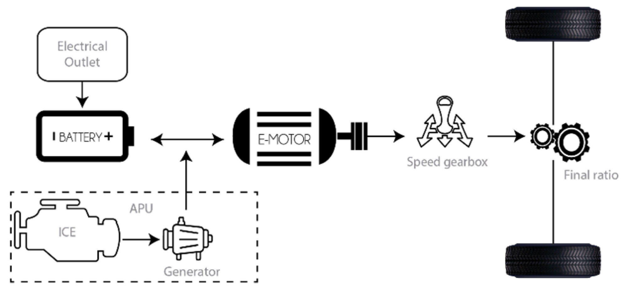
1.1. Energy of Extended-Range Electric Vehicles

Energy analysis is crucial for understanding the efficiency advantages of EREVs and for the proper design and evaluation of energy management strategies. In EREVs, the total power demand is met by batteries or other storage devices through electric pathways. There are two distinct energy flows: First, we have the state of charge (SOC) of the battery, which typically comes from the electrical grid and is used by the electric machine to propel the vehicle. The internal combustion engine (ICE) drives a generator that produces energy, which can be used to (i) charge the battery; (ii) maintain the SOC of the battery; or (iii) directly power the electric motor with the energy generated. In the last scenario, the energy demanded by the electric motor must be precisely matched and consistently supplied by the generator.

Figure 2 illustrates the three modes of operation: (a) discharge mode, where only the battery supplies power; (b) charge mode, where the generator recharges the battery; and (c) stable mode, where the generator powers the electric motor while the battery maintains its SOC.

1.2. Equivalent Consumption Minimization Strategy Application in EREVs

Regardless of the powertrain configuration, the core challenge in controlling Hybrid Electric Vehicles (HEVs) lies in the real-time management of power flows from energy converters to meet control objectives. A key feature of this challenge is that the control objectives are typically integral (e.g., fuel consumption or hydrogen consumption [52]) or semi-local in time, such as drivability, whereas the control actions occur at specific moments in time. Additionally, these control objectives are often bound by integral constraints, like maintaining the battery’s SOC within a designated range. Generally, the energy management problem in a hybrid vehicle can be formulated as an optimization problem over a finite time horizon [53]. The solution to this problem can be derived using optimal control theory methods, which aim to identify a control strategy that satisfies an optimality criterion, typically defined as an integral performance index over a specified time period [54].

1.3. Problem Formulation

The supervisory control problem is defined with the goal of minimizing the total fuel volume $V_f$ during a driving mission. In EREVs, the internal combustion engine is solely responsible for powering the generator/alternator. Therefore, the optimal energy management challenge in an EREV involves determining the control function $u\left(t\right)$ that reduces the fuel consumption $V_f$ over the duration of a driving cycle $t_f$. This is equivalent to minimizing the following integral performance index:

$$J={\int }_0^{t_f}{\dot{V}}_f(u\left(t\right),t)dt$$

(1)

Here, $\dot{V_f}$ represents the fuel consumption rate. The minimization of J is the core of the so-called equivalent consumption minimization strategy (ECMS), which can be formulated also in terms of a fuel equivalent mass flow rate [55]. The problem is constrained by factors such as the physical limits of the actuator, the available energy stored in the batteries, and the need to keep the battery SOC within specified boundaries [56]. These considerations turn the optimal energy management task into a constrained, finite-time optimal control problem, where the objective function is minimized while adhering to a combination of local and global constraints on the state and control variables as detailed below.

1.3.1. Global Constraints

The final SOC must achieve a specified target value: $x\left(t_f\right)=x_{target}$. In other words, it is necessary that

$$\Delta x=x\left(t_f\right)-x_{target}=0$$

(2)

In charge-sustaining mode, the net energy drawn from the battery should be zero over the course of a given driving mission, meaning that the SOC at the end of the driving cycle $x\left(t_f\right)$ should match the SOC at the start. In cases where battery depletion is desired, the target SOC value may be lower than the initial one. Equation (2) establishes the global state constraints for the control problem, primarily to ensure that different solutions can be compared fairly by having them start and end with the same battery energy level. In real-world vehicle applications, it is typically sufficient to maintain the SOC within a certain range, as a slight difference between the desired and actual SOC at the end of a cycle is acceptable and does not impact the vehicle’s functionality.

1.3.2. Local Constraints

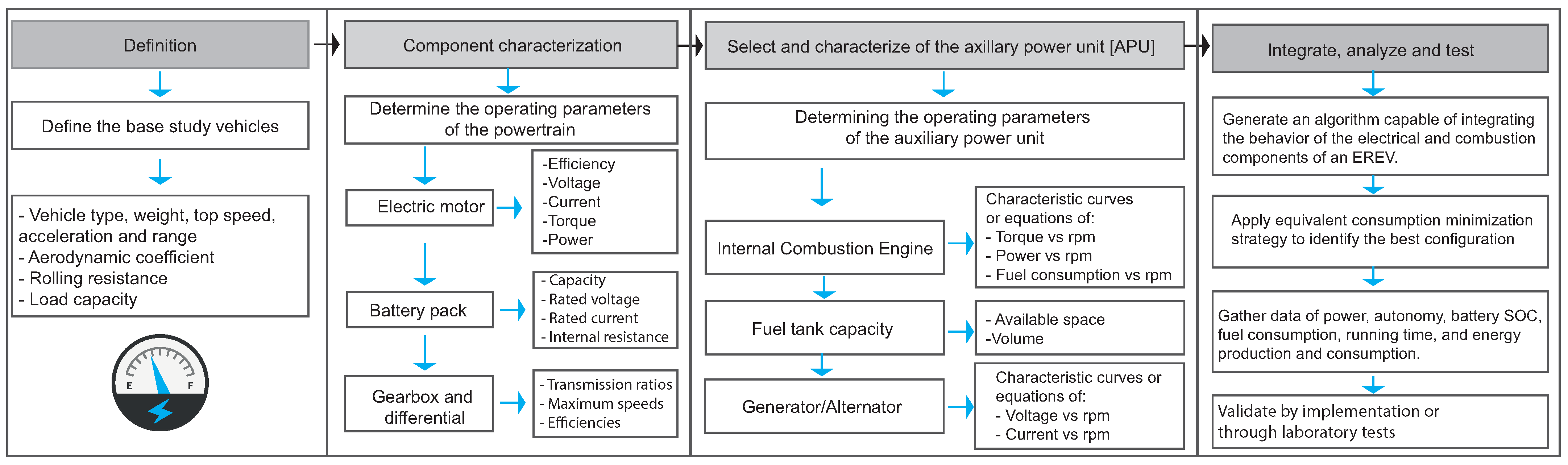
Local constraints are applied to both the state and control variables. The local (or instantaneous) constraints on the state refer to the requirement that the state of charge must stay within a specified maximum and minimum range to ensure high battery efficiency and prolong its cycle life. Meanwhile, the local constraints on the control variables are established to ensure that the system operates within its physical limits, such as the maximum and minimum torque and speed of the engine, motor, and generator, as well as the battery’s power output.

The local constraints are

$$\begin{array}{c}SO{C}_{minimum}\le SOC\left(t\right)\le SO{C}_{maximum}\end{array}$$

(3)

$$\begin{array}{c}{P}_{battery,minimum}\le P_{battery}\left(t\right)\le P_{battery,maximum}\end{array}$$

(4)

$$\begin{array}{c}{T}_{x,minimum}\le T_x\left(t\right)\le T_{x,maximum}\end{array}$$

(5)

$$\begin{array}{c}{\omega }_{x,minimum}\le {\omega }_x\left(t\right)\le {\omega }_{x,maximum}\end{array}$$

(6)

$$\begin{array}{c}{V}_{x,minimum}\le V_x\left(t\right)\le V_{x,maximum}\end{array}$$

(7)

where bounds ($minimum,maximum$) are set for the state of charge ($SOC$), battery power ($P_{battery}$), torque (T), angular speed ($\omega$) and equivalent volume of fuel (V). The subscript x denotes the device, engine, or generator.

2. Methodology

The limited range of electric vehicles, combined with the cost and weight of batteries, poses a challenge to their widespread adoption. Simply increasing the number of batteries without careful consideration may not significantly improve the vehicle’s range and can even be counterproductive. Therefore, we explore various methods to extend the range of electric vehicles by integrating real-time charging technologies in a series configuration. The electric motor, responsible for powering the wheels, operates at its maximum efficiency, while the range extender focuses solely on charging the batteries and operates at its highest efficiency regimes. Through this analysis, we identify the most effective approach for extending the range [57].

In the design of an electric vehicle, determining the appropriate battery size and selecting the electric motor (and possibly a transmission system) are critical factors. The electric motor delivers the power needed to drive the vehicle, while the battery size is chosen based on the desired range. Initially, we investigate the integration of a gearbox and differential to optimize the electric motor’s efficiency range, recognizing that the powertrain of conventional ICE vehicles was not originally designed to work with electric motors [51].

Hybrid vehicles (HVs) provide more design flexibility than conventional or fully electric vehicles, enabling the propulsion system and architecture to be customized according to the vehicle’s intended use. For series hybrids or Extended-Range Electric Vehicles (EREVs), the key challenge is to determine the optimal power source, whether from the internal combustion engine or the energy storage system to power the electric motor. The goal is to maximize fuel efficiency and minimize emissions.

The auxiliary power unit (APU) is optimized for maximum energy efficiency, employing strategies to minimize fuel consumption and reduce emissions from the combustion engine driving the generator. The energy generated for battery charging is thoroughly analyzed using simulations in MATLAB-Simulink R2024a, and the obtained data are validated for accuracy. Furthermore, we propose a model to size a powertrain for Extended-Range Electric Vehicles, harnessing the high efficiency of the electric motor for wheel propulsion and the APU capabilities to charge batteries, thereby increasing the vehicle’s autonomy with minimal fuel consumption and emissions. These steps successfully fulfill the objectives of this research; see Figure 3.

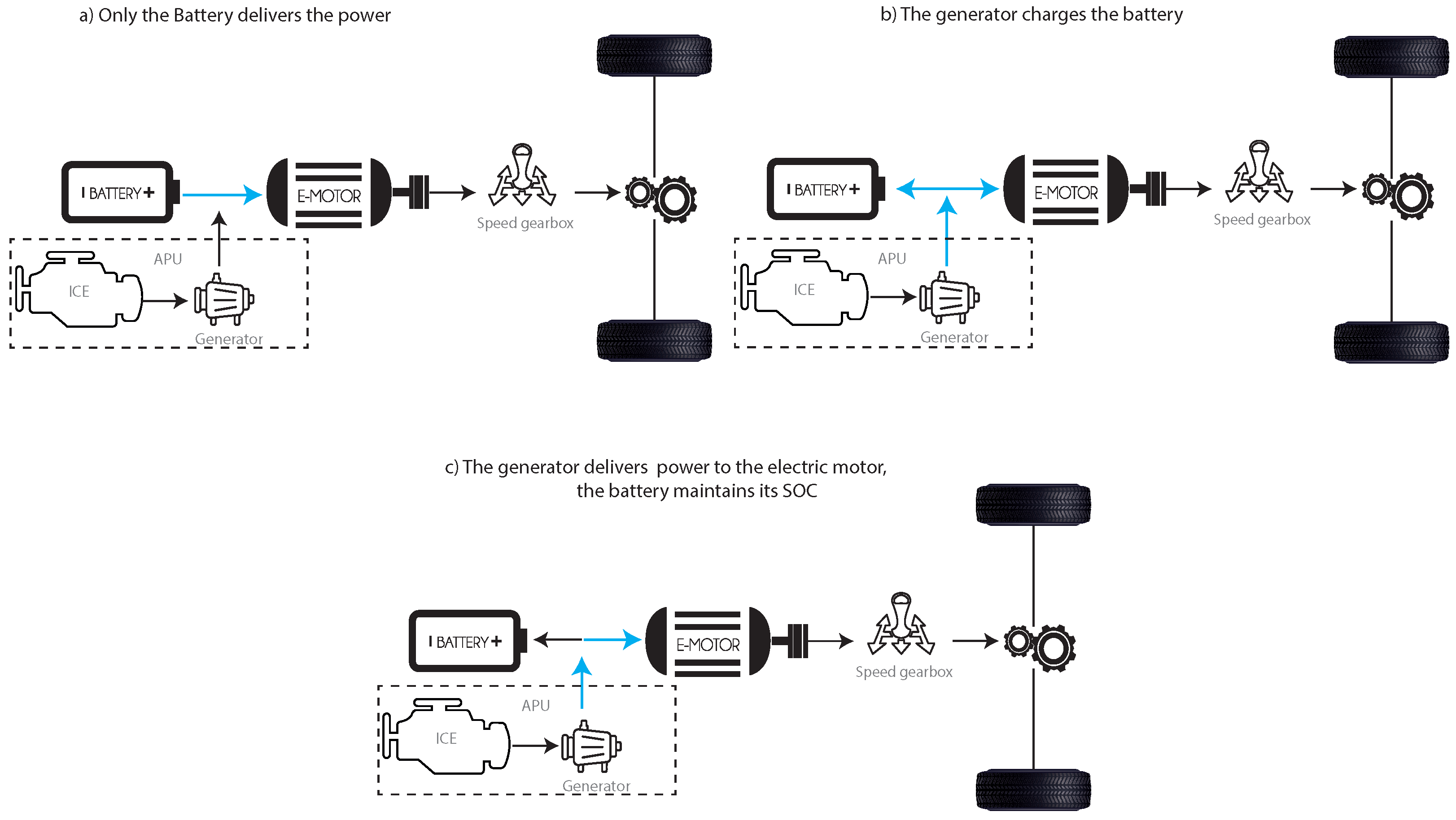
2.1. Algorithm Usage Scenarios

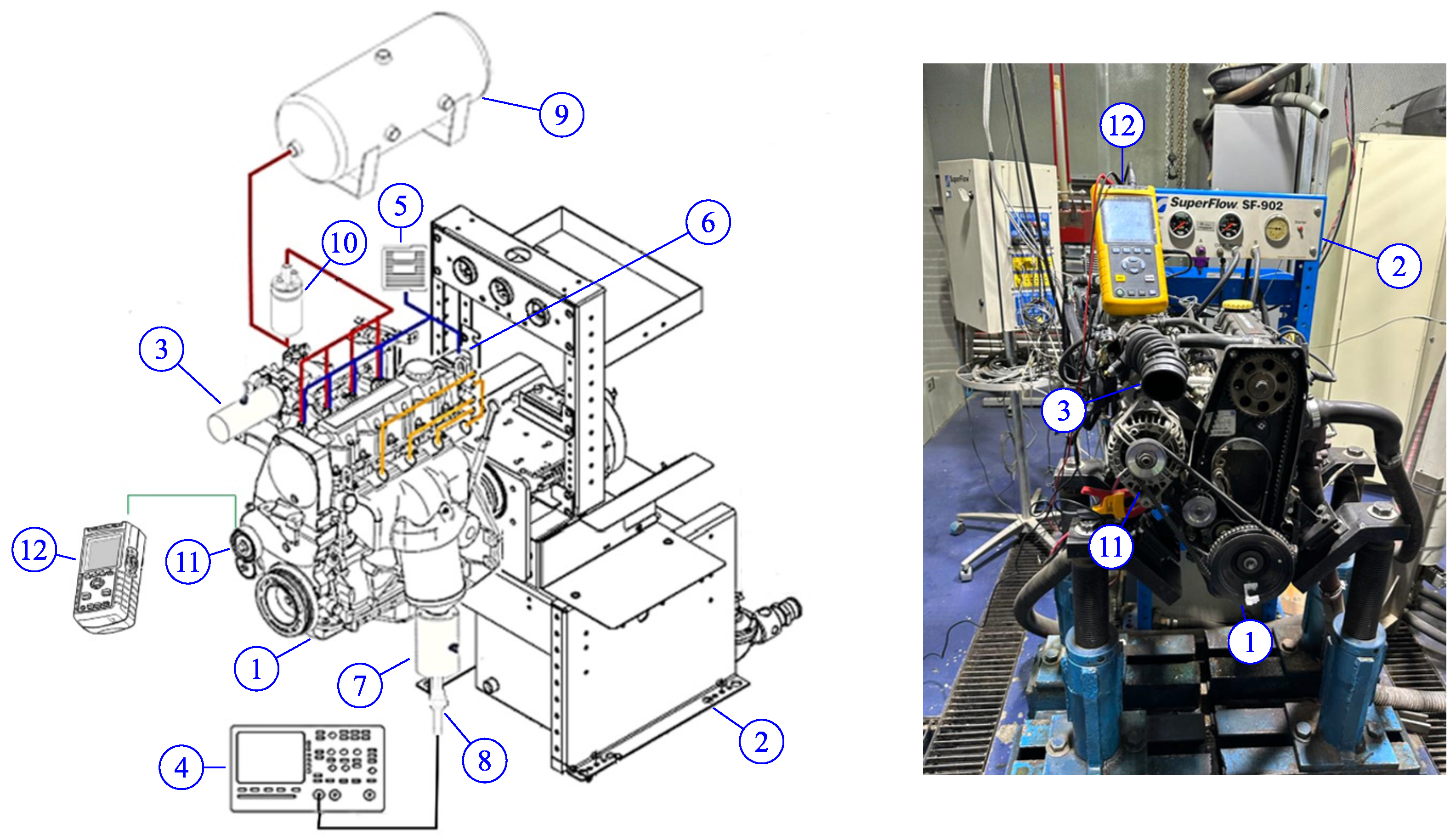
When simulating the range of an Extended-Range Electric Vehicle, there are several variables that can influence its performance. In the following concept map, different scenarios are analyzed, where the real part is considered at the moment of performing cycles in real conditions, or in some cases, predefined cycles to analyze specific consumption, depending on the variables that are taken into account. It is necessary to consider an acceptable range of these variables because although tests are performed in defined routes, many times, these vary even if they are controlled, for example, traffic, road environment [58], weather conditions [59], ambient temperature, the use of auxiliary systems, driving modes [60]. These scenarios can vary and have to be considered when performing these tests, unlike if they are performed at the laboratory level where the tests are more controlled but certain variables are neglected or certain assumptions are made. Figure 4 is a conceptual map showing all possible scenarios and their actual variations.

2.2. Test Setup

The testing protocol was conducted using the chassis and engine dynamometer platforms at the Automotive Mechatronics Research Center (CIMA) at Tecnológico de Monterrey. In this setup, a driving cycle speed profile is artificially simulated on the vehicle. Simultaneously, key data are collected from the vehicle to assess its range, energy consumption, acceleration, speed, and power (both mechanical and electrical), among other important metrics.

2.3. Physical Implementation

After integrating the mathematical models, various simulations were conducted by adjusting the angular speed of the APU (ICE generator) to create an efficiency map. Additionally, the implementation of ECMS control was used to enhance energy generation. The powertrain optimization was carried out in a practical manner.

2.4. Data Acquisition

In this study, data collection was conducted using the DEWESOFT SIRIUS XHS data acquisition system. This equipment allows for the real-time measurement of current and voltage during various driving cycles. The chassis dynamometer, AUTODYN 30, was employed to measure power and torque. The SIRIUS XHS system offers high-speed data acquisition (up to 15 MS/s), with interfaces such as USB 3.0, GLAN, and CAN, providing flexible connectivity.

The AUTODYN 30 dynamometer features a peak power capacity of 2500 HP, a maximum speed of 225 mph, and the capability to measure energy consumption during standardized driving cycles. It is also used to evaluate power and torque at the wheels of the electric vehicle and the energy consumed at constant speeds.

For internal combustion engine (ICE) and generator characterization, the SUPERFLOW SF902 engine dynamometer was utilized as shown in Figure 5. This equipment measures torque, power, and fuel consumption across different loads, with features including a maximum absorber speed of 10,000 rpm and a torque range of 0–1000 lb-ft. Additionally, a Fluke 43b power quality analyzer was used to measure and store current and voltage data for the generator and alternator, with maximum operating voltages of 5000 V and currents of up to 500 kA.

This comprehensive setup enabled detailed characterization of the electric vehicle, ICE, and generator, ensuring the accurate measurement of mechanical and electrical parameters essential for performance analysis.

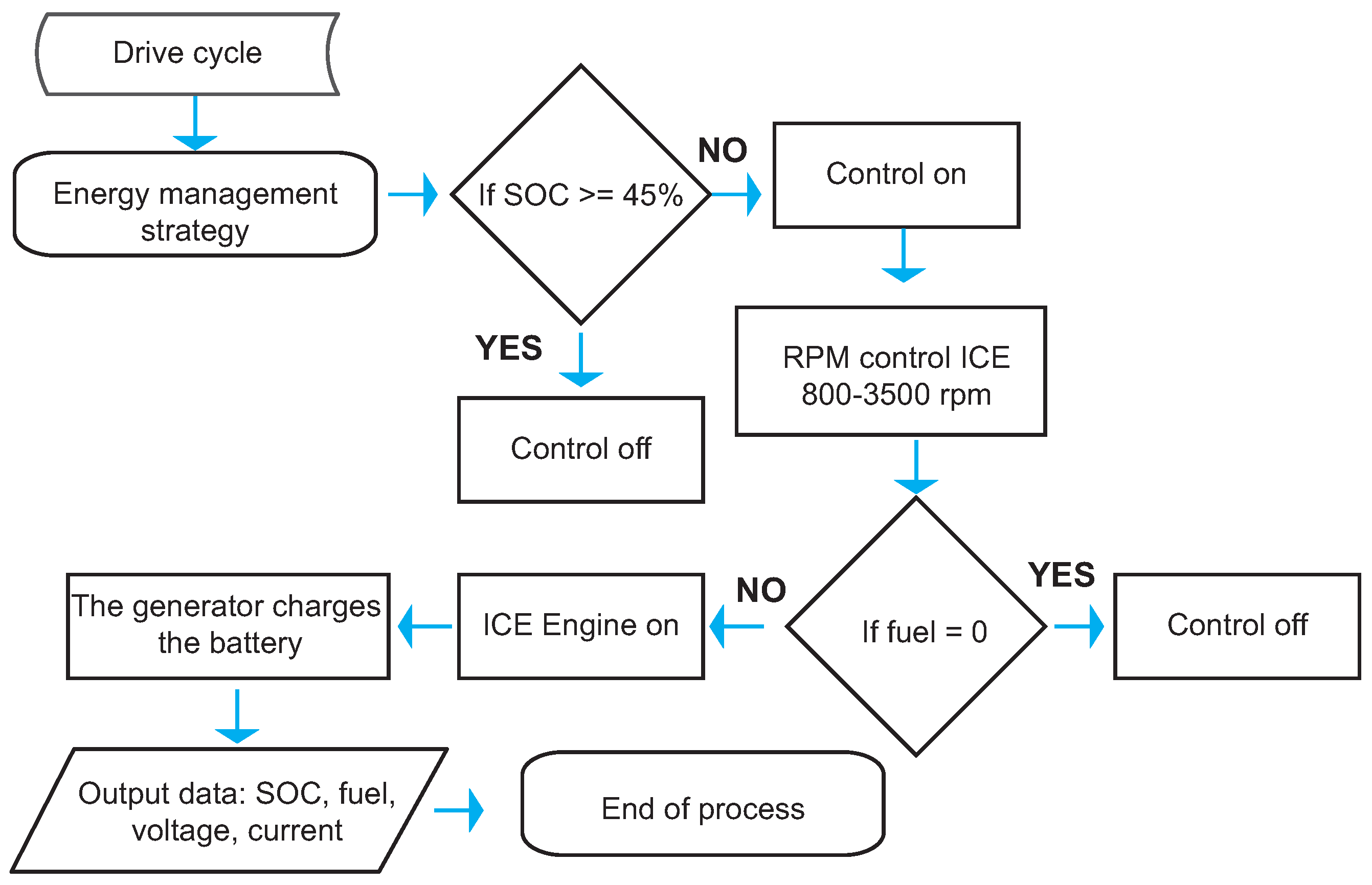
2.5. ECMS-Based Supervisory Control

The Equivalent Consumption Minimization Strategy (ECMS) is a heuristic approach used to tackle the optimal control problem, making it an effective solution for managing energy in HEVs [61]. ECMS simplifies the global minimization problem by solving it at each moment based on the current energy flow within the powertrain.

The ECMS operates on the principle that, in charge-sustaining Extended-Range Electric Vehicles or series hybrid vehicles, the difference between the initial and final state of charge of the battery is minimal and negligible relative to the total energy consumed. This implies that the electrical energy storage system functions merely as an energy buffer; ultimately, all energy originates from fuel, and the battery acts as an auxiliary, reversible fuel tank. Any electrical energy used during the battery discharge must later be replenished either by engine fuel or regenerative braking.

At any given operating point, two scenarios are possible. If the battery power is positive (discharge case) at the current moment, this indicates that the battery will need to be recharged later, leading to additional fuel consumption. The amount of fuel required to restore the battery to its desired energy level depends on (1) the engine’s operating condition at the time of recharging and (2) the amount of energy that can be recovered through regenerative braking. Both factors, in turn, depend on the vehicle’s load and the driving cycle.

By converse, if the battery power is negative (charge case), the stored electrical energy will reduce the engine load necessary to meet the vehicle’s road load, resulting in immediate fuel savings. However, substituting electrical energy for fuel energy also depends on the load imposed by the driving cycle.

The ECMS approach is based on the principle that a cost is assigned to electrical energy, making the stored electrical energy equivalent to consuming (or saving) a certain amount of fuel. Although this cost is not directly known since it depends on future vehicle behavior—it has been shown that it can be broadly related to driving conditions. When implementing ECMS, the use of stored electrical energy is accounted for in terms of chemical fuel usage (g/s), allowing for the definition of an equivalent fuel consumption that considers the cost of electricity [62,63]. The key concept of ECMS is that, in sustain mode, equivalent fuel consumption can be linked to the use of electrical energy.

2.6. Control Integration

For using the ECMS, it is important to highlight that the revolutions at which the internal combustion engine rotates directly influence the energy produced and fuel consumption. Therefore, the objective is mainly to reduce fuel consumption and generate the greatest amount of energy, which in this case would become the equivalent energy that can be obtained with adequate control of the engine and the generator or alternator. To meet this objective, and under the previous simulations, it is possible to observe that the revolutions at which the greatest amount of energy is obtained with the least consumption are between 1000 and 3500 rpm. For this, the state of charge will be stabilized in a percentage initially established by the controller, and depending on the driving cycle, the control will vary the revolutions of the engine and the generator/alternator depending on the SOC. To summarize, the SOC will feed the control, and the control will send the motor the revolutions at which it must work depending on the consumption and discharge of the batteries. To stabilize the SOC and control the engine with the necessary revolutions at which the generator/alternator will deliver the greatest energy depending on the requirement of the driving cycle, a PID control will be used; in this case, I specify only the proportional (P) and it will contain a saturation between 1000 and 3500 rpm. To verify the thesis that adequate control can improve consumption and generate more energy, the strategy mentioned above is applied, and simulations are carried out in the NEDC management cycle, WLTC-2 and WLTC-3. The results are shown below in the next section, and they are compared to the largest generation of energy without control and the application of the strategy. The flowchart with which the control works is fed directly with the SOC of the battery and tries to keep the defined SOC as stable as possible by varying the engine revolutions, and this generated energy feeds the batteries; the amount of fuel is sensed second by second, and when it is finished, the engine stops running and the APU shuts down. See Figure 6.

3. Experimental Test Vehicle

The experimental platform for this work is an electric vehicle (Van type) assembled in Mexico, available at the Research Center for Automotive Mechatronics (CIMA). This electric vehicle, named GMTA-E1, is currently used as a taxi in Mexico City. Utilizing an electric configuration for public transportation vehicles helps reduce emissions compared to those produced by internal combustion vehicles. Additionally, a city vehicle maintains high efficiency at low rpm, making it ideal for urban operations.

The electric vehicle operates when the driver presses the accelerator pedal, which triggers a torque setpoint request for the induction machine’s power stage. This stage consists of a three-phase voltage inverter that requires a constant voltage and variable current from the battery management system (BMS). From an energy perspective, the electric motor converts electrical energy into mechanical energy. This rotational energy is then transferred through the gearbox to the differential, eventually reaching the rear wheels and resulting in the vehicle’s longitudinal motion. The auxiliary power unit (APU) extends the vehicle’s range by charging the batteries when activated. The developed control functions regulate the speed at which the internal combustion engine (ICE) operates.

In the test conducted on a chassis dynamometer, it is observed that the torque curve of the electric motor peaks around 846.8 rpm with approximately 512.865 Nm. From this point, the torque gradually decreases as the rpm increases, reaching approximately 31.995 Nm at 4000 rpm. The power curve shows a constant increase, reaching a maximum of 23 hp around 2000 rpm. Subsequently, the power experiences a slight decline and remains stable at around 10.3 hp at 3078.1 rpm, ending with a power of approximately 3.8 hp at 4000 rpm as seen in Figure 7.

The powertrain for the experimental test vehicle was chosen with the goal of creating an affordable utility transport vehicle, which required the use of a small motor. The powertrain features a central induction electric motor with a nominal output of 15 hp. This motor is a three-phase, four-pole unit that is mechanically connected to a five-speed gearbox. The gearbox is then connected to a differential on the rear axle, which transfers power to the wheels. The electric motor operates within a voltage range of 96 to 220 V and is powered by a 32 kW battery pack with a nominal voltage of 105 V, ensuring it stays within the motor’s operating range and provides the necessary energy for efficient performance. The complete vehicle specifications are summarized in

Table 2. Vehicle features.

Description	Symbol	Unit	Value
Powertrain configuration	−	−	Central electric motor with
			five-speed transmission and
			final drive ratio
Vehicle mass	m	$\mathrm{kg}$	1370
Battery pack capacity	−	$\mathrm{kWh}$	32 (Li-ion cells)
Nominal voltage	$E_0$	$\mathrm{V}$	105
Maximum capacity	Q	$\mathrm{Ah}$	304
Initial state-of-charge	−	%	100
Internal resistance	$\mathsf{\Omega }$	$\mathrm{Ohms}$	0.07
Nominal current discharge	i	$\mathrm{A}$	160
Exponential voltage	$\alpha$	$\mathrm{V}$	106
Exponential capacity	$\beta$	$\mathrm{Ah}$	260
Frontal area	A	${\mathrm{m}}^2$	2.15
Drag coefficient	$C_d$	−	0.436
Rolling resistance coefficient	${\mu }_{rr}$	−	$0.015$
Gearbox efficiency	${\eta }_g$	−	0.95
First shift ratio	${ϵ}_{g,1}$	−	3.636
Second shift ratio	${ϵ}_{g,2}$	−	1.9641
Third shift ratio	${ϵ}_{g,3}$	−	1.428
Fourth shift ratio	${ϵ}_{g,4}$	−	1
Fifth shift ratio	${ϵ}_{g,5}$	−	0.801
Final ratio efficiency	${\eta }_d$	−	0.95
Final ratio	${ϵ}_d$	−	4.3
Maximum torque	−	$\mathrm{Nm}$	691.51
Maximum power	−	$\mathrm{kW}$	25.92
Maximum speed	−	$\mathrm{km}/\mathrm{h}$	117

. These parameters were determined through dedicated characterization experiments using CIMA’s laboratory equipment, including a chassis dynamometer.

The experimental section of the vehicle is divided into two primary parts. The first part involves testing and characterizing the vehicle to develop an accurate mathematical model and validate its precision. The second part focuses on characterizing the auxiliary power unit (APU), which in this case is an internal combustion engine. With both the vehicle and APU characterized and the mathematical model validated, the integration of the APU into the vehicle will be simulated. This simulation will enable the assessment of improvements in the vehicle’s range and the application of control strategies designed to optimize efficiency, extend range, and reduce fuel consumption of the internal combustion engine. This procedure follows the previously outlined methodology.

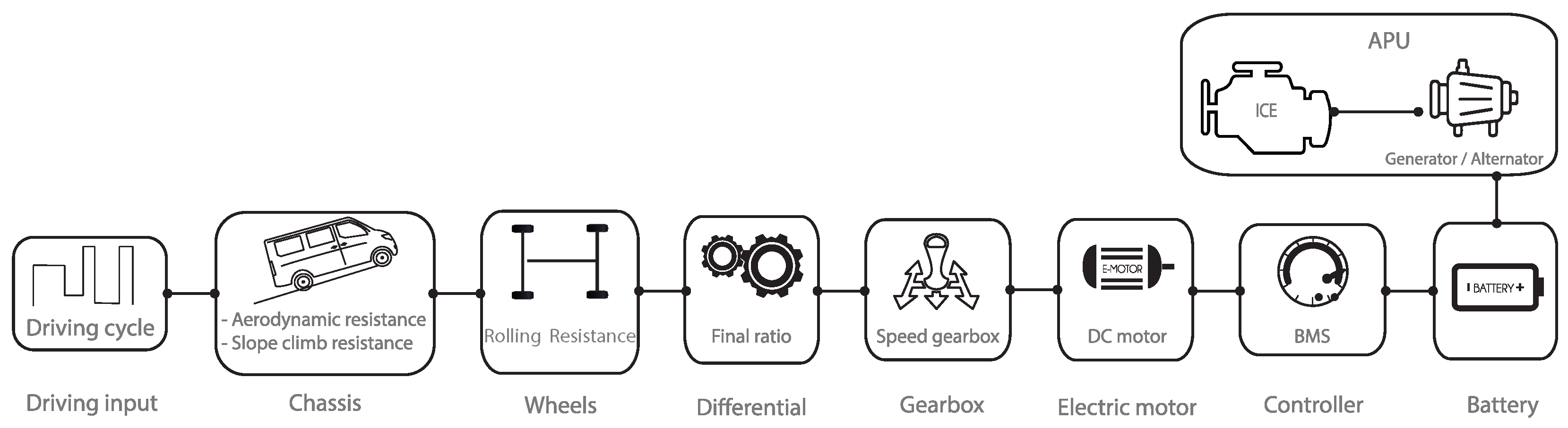
3.1. Electric Vehicle Model Development: Vehicle Dynamics

The longitudinal dynamics of the vehicle focus solely on the control actions related to throttle and braking, while the vertical, lateral, and roll dynamics are not considered. The force propelling the vehicle forward must counteract several resistances, including rolling resistance, aerodynamic drag, gravitational force when driving on an incline, and inertial forces during changes in vehicle speed.

In the context of longitudinal dynamics, these forces are crucial, as they dictate the energy required to maintain or alter the vehicle’s speed. Rolling resistance is primarily due to the friction between the tires and the road surface, and it increases with vehicle weight and tire deformation. Aerodynamic drag, which grows with the square of the vehicle’s speed, resists forward motion and is influenced by the vehicle’s shape, frontal area, and drag coefficient. When the vehicle encounters a slope, the component of its weight along the incline either aids or opposes motion, depending on whether the vehicle is moving uphill or downhill. Lastly, inertial forces come into play during acceleration or deceleration, requiring additional power to change the vehicle’s speed.

This scenario is illustrated in the free-body diagram in Figure 8. where each of these forces is represented. Below, we detail each contributing factor and describe the tests conducted to identify the relevant parameters affecting the vehicle’s longitudinal dynamics.

3.1.1. Rolling Resistance Force

Rolling resistance force arises from the friction between the vehicle’s tires and the road surface. This force can be quantified using the following equation:

$$F_{rr}={\mu }_{rr}mg$$

(8)

where ${\mu }_{rr}$ represents the rolling resistance coefficient, m is the vehicle’s mass, and $g=9.81\mathrm{m}/{\mathrm{s}}^2$ is the acceleration due to gravity. The rolling resistance coefficient ${\mu }_{rr}$ is a dimensionless value that characterizes the tire–road interaction and depends on several factors, including tire composition, tread design, inflation pressure, and the roughness of the road surface. A higher ${\mu }_{rr}$ indicates greater resistance, which results in more energy required to overcome this force, thus reducing the vehicle’s efficiency.

To accurately determine ${\mu }_{rr}$ for the vehicle in question, we adhered to the guidelines set by the International Organization for Standardization (ISO) for the experimental calculation of rolling resistance [64].

3.1.2. Aerodynamic Drag

Aerodynamic drag is a critical force that opposes a vehicle’s motion as it moves through the air. This force becomes increasingly significant at higher speeds, as it grows with the square of the vehicle’s velocity. Reducing aerodynamic drag is essential for improving fuel efficiency and extending the range of both conventional and electric vehicles.

The aerodynamic drag force can be calculated using the following equation:

$$F_{ad}={\displaystyle \frac{1}{2}}\rho A{C}_d{v}^2$$

(9)

Being that $\rho =1.225\mathrm{kg}/{\mathrm{m}}^3$ is the density of the air, $C_d$ is the aerodynamic drag coefficient, A is the frontal area of the vehicle, and v is the vehicle’s longitudinal speed. The aerodynamic drag coefficient $C_d$ is a dimensionless value that represents the effectiveness of the vehicle’s shape in reducing air resistance. A lower $C_d$ indicates a more aerodynamically efficient design, resulting in less drag and improved vehicle performance. The frontal area A is the projected area of the vehicle’s front-facing surface, which directly influences the magnitude of the drag force.

In this analysis, the aerodynamic drag coefficient $C_d$ was determined using computational fluid dynamics (CFD) simulations, which provide detailed insights into how air flows around the vehicle’s body. These simulations are crucial for optimizing the vehicle’s shape to minimize drag. The frontal area A was measured based on the vehicle’s dimensions, allowing for an accurate calculation of the drag force.

3.1.3. Hill Climbing Force

The hill climbing force refers to the force required to propel a vehicle uphill on a sloped road. This force is particularly important in scenarios where the vehicle must overcome gravity to maintain its motion on an incline. The hill climbing force can be calculated using the following equation:

$$F_{hc}=mgsin\psi$$

(10)

where m is the vehicle’s mass, g is the acceleration due to gravity, and $\psi$ is the angle of the road slope.

3.1.4. Net Force

To determine the vehicle’s acceleration, Newton’s second law can be applied by first calculating the net thrust of the car as a function of its speed. It is important to recognize that the vehicle’s translational motion is inherently linked to the rotational movement of components connected to the wheels, such as the engine and the driveline. As a result, any change in the vehicle’s translational speed will be accompanied by a corresponding change in the rotational speed of these components.

To account for this coupling, a mass factor, denoted as ${\gamma }_m$, is introduced into the equation for vehicle acceleration a [65]. This factor incorporates the effect of the inertia of the rotating parts on the vehicle’s acceleration characteristics. The resulting equation for the net force $F_{net}$ is expressed as

$$F_{net}={\gamma }_{m}ma$$

(11)

Here, ${\gamma }_m$ can be calculated based on the moments of inertia of the rotating components, including the wheels, gearbox gears, and differential. This factor is crucial because it adjusts the effective mass of the vehicle to account for the additional inertia due to these rotating parts, which can significantly influence the acceleration performance.

For passenger cars, the mass factor ${\gamma }_m$ can be estimated using the following equation:

$${\gamma }_m=1.04+0.0025{\left({ϵ}_g{ϵ}_d\right)}^2$$

(12)

In this equation, the first term on the right-hand side represents the contribution of the wheels’ rotating inertia, while the second term accounts for the inertia of components rotating at the engine’s equivalent speed, factoring in the overall gear reduction. Here, ${ϵ}_g$ represents the gearbox ratio, and ${ϵ}_d$ denotes the differential or final drive ratio.

Understanding and accurately calculating the mass factor is essential for predicting vehicle performance, particularly during acceleration. The influence of rotating components’ inertia can impact the responsiveness of the vehicle, especially in scenarios requiring rapid acceleration. This consideration is vital in the design and tuning of vehicles, where the balance between the power delivery and efficient acceleration is critical for achieving optimal performance and driving experience.

3.1.5. Tractive Force

The tractive force is the total force required to propel the vehicle forward and is calculated by summing the contributions of various forces acting on the vehicle. These forces include the net force ($F_{net}$), the hill climbing force ($F_{hc}$), the aerodynamic drag force ($F_{ad}$), and the rolling resistance force ($F_{rr}$). The equation for tractive force is expressed as

$$F_t=F_{net}+F_{hc}+F_{ad}+F_{rr}$$

(13)

This combined force represents the total effort needed to overcome all forms of resistance and inertia that oppose the vehicle’s motion.

Once the tractive force is determined, it can be converted into the power required to maintain the vehicle’s speed. The power needed at the wheels, also known as the mechanical power, is given by

$$P_m=F_{t}v$$

(14)

where v is the vehicle’s speed.

Understanding the tractive force and the corresponding power requirement is critical for vehicle design and performance evaluation. The tractive force must be sufficient not only to overcome resistive forces but also to provide the necessary acceleration and maintain the desired speed, especially under varying road conditions such as inclines or during high-speed driving.

3.1.6. Gradability

Gradability refers to the steepest incline a vehicle can successfully climb at a constant speed. When a vehicle ascends a slope at a steady pace, the tractive effort must counteract multiple forces, including grade resistance, rolling resistance, and aerodynamic drag. For relatively small slope angles $\psi$, it is often assumed that $tan\psi \approx sin\psi$. By applying this approximation and solving for $\psi$ in the hill climbing force Equation (10), the maximum gradability is

$${\psi }_{max}=arcsin\left({\displaystyle \frac{P_m{\eta }_t}{mgv}}-{\displaystyle \frac{\rho A{C}_d{v}^2}{2mg}}-{\mu }_{rr}-{\displaystyle \frac{{\gamma }_{m}a}{g}}\right)$$

(15)

In this equation, ${\psi }_{max}$ represents the maximum slope angle that the vehicle can ascend. The term $P_m$ is the power produced by the engine or motor, and ${\eta }_t$ is the efficiency of the drivetrain, which includes losses due to friction and other mechanical inefficiencies.

Gradability is a critical performance metric, especially for vehicles that operate in hilly or mountainous regions. A vehicle’s ability to climb steep grades without losing speed is not only a measure of engine power but also a reflection of the overall efficiency of the powertrain and the vehicle’s design.

3.2. Battery Model

The battery in the system, a lithium-ion (Li-ion) cell pack, is modeled by its state of charge (SOC), which represents the amount of energy stored in the battery. The SOC is a dimensionless quantity, where $SOC=1$ indicates a fully charged battery and $SOC=0$ signifies a completely depleted battery. During a driving cycle, the energy flowing into the battery (charging, $f_c$) and out of the battery (discharging, $f_{dc}$) is calculated at each time step using the following equations:

$$\begin{array}{cc}\hfill f_{dc}& =E_0-K{\displaystyle \frac{Q}{Q-it}}{i}^{*}-K{\displaystyle \frac{Q}{Q-it}}it+\alpha {\mathrm{e}}^{-\beta it}\hfill \end{array}$$

(16)

$$\begin{array}{cc}\hfill f_c& =E_0-K{\displaystyle \frac{Q}{it+0.1Q}}{i}^{*}-K{\displaystyle \frac{Q}{Q-it}}it+\alpha {\mathrm{e}}^{-\beta it}\hfill \end{array}$$

(17)

In these equations, t represents time, $E_0$ is the nominal voltage of the battery, and K is the polarization constant, which accounts for voltage drops due to internal resistance and other factors. The term i is the instantaneous current drawn from or supplied to the battery, whereas $i^{*}$ is the current filtered through a low-pass filter with a time constant $\tau =10\mathrm{s}$. Q is the maximum capacity of the battery, and $\alpha ,\beta$ are voltage and capacity exponents, respectively.

3.3. Auxiliary Power Unit Characterization

The auxiliary power unit (APU) comprises an internal combustion engine (ICE) paired with a generator. This system extends the range of the electric vehicle by supplying extra energy to either recharge the battery or maintain the state of charge (SOC) while the vehicle is in use.

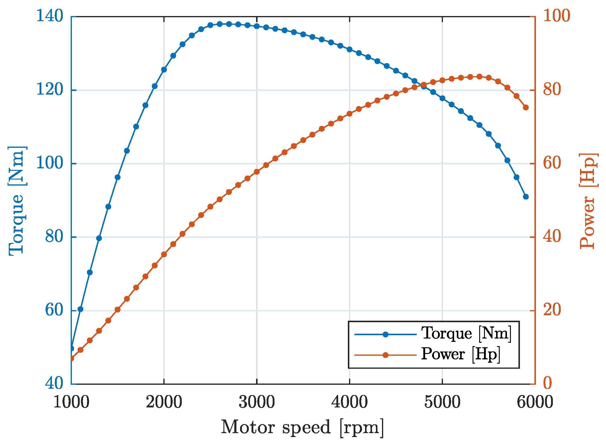
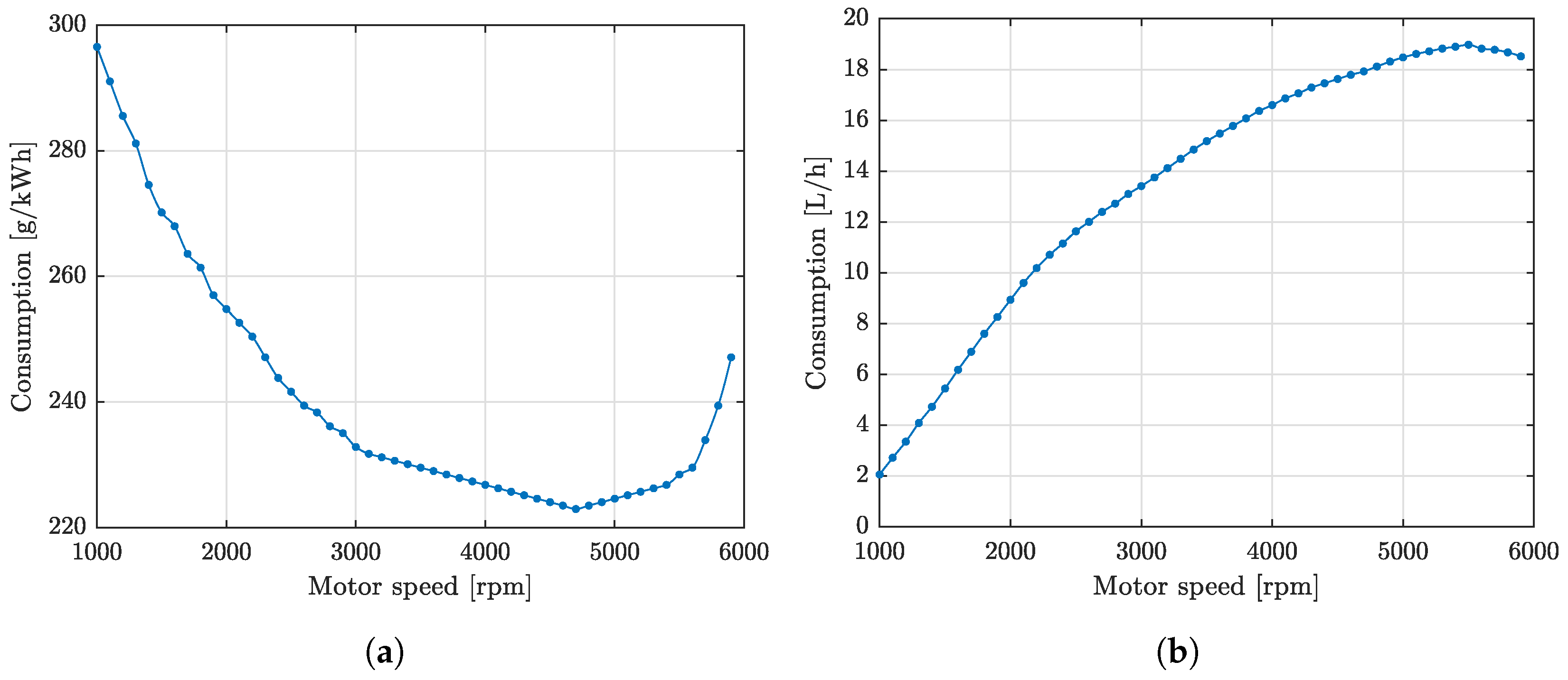
3.3.1. Internal Combustion Engine Characterization

The engine model includes torque, power, and fuel consumption. The engine map documents specific engine characteristics as a function of the operating point. This representation may include discrete values at individual points. In Figure 9, the torque and power characteristics curves of the Z16SE engine for a range extender in a series Hybrid Electric Vehicle are depicted. Additionally, Figure 10a illustrates the specific fuel consumption in relation to the speed of the Z16SE engine. These data are intended for use in extending the range in the EREV model. The expressed value is linked to the energy function per a certain amount of grams, which, in turn, is influenced by the motor’s rotational speed (angular speed).

Fuel consumption varies depending on the revolutions; consumption is often higher when driving at low revolutions, whereas at high revolutions, the consumption tends to be lower, between 2500 and 3500 rpm. Of course, this significantly depends on the engine being analyzed.

The static map approach assumes that the engine operates as an ideal actuator, responding instantly to input commands. To determine the theoretical maximum fuel consumption, the following expression is utilized:

$$Q_{fuel,max}={\displaystyle \frac{N{q}_{esp}}{\rho }}$$

(18)

where $Q_{fuel}$ is the maximum fuel consumption of the engine operation at maximum output, N is the engine power, $q_{esp}$ is the specific fuel consumption for N, and $\rho$ is the fuel density. For gasoline, the density is 743 kg/m³ [66].

Figure 10b shows the theoretical maximum fuel consumption of the Z16SE at different speed engines. These values were calculated with expression (12), and all the data used were referred from Figure 10a.

In the model developed in MATLAB-Simulink, the function used to represent the fuel consumption is given by

$$Q_{fuel}=-8·{10}^{-7}{\omega }^2+9.2·{10}^{-3}\omega -6.4431$$

(19)

where the angular speed $\omega$ is expressed in rpm.

3.3.2. Generator Characterization

The wires through which the current and voltage circulate were located, and the engine speed was varied. As a result, the characteristic curves of both voltage and current versus revolutions were obtained. The generator model is an AC generator, and the voltage curve is shown in Figure 11a; the current and voltage multimeter are automatically set to measure AC voltage. Commercially, the generator has an identification code PM0102500.

A logarithmic trendline was used to describe the generator voltage according to the data obtained with an accuracy of 98.3%:

$$e_g=297.19{log}_{10}\left(\omega \right)-2333.9$$

(20)

Similarly, the generator current was measured (see Figure 11b) and approximated through the following function:

$$i_g=-1·{10}^{-6}{\omega }^2+0.0178\omega -44.419$$

(21)

In this case, due to the data discrepancy between 4500 and 6000 rpm, the best trendline with a high degree of accuracy was a second-degree polynomial with an accuracy of 93.5%. Equations (20) and (21) will be used whenever the AC generator is employed in the system.

3.4. Internal Combustion Engine and Generator Sizing

When sizing an internal combustion engine and a generator, the key consideration is the amount of additional energy required to enhance autonomy. Firstly, the generator must be sized to produce this extra energy, taking into account the resistance it will impose on the internal combustion engine. This step ensures that the generator can meet the energy demand and properly interact with the engine. The second crucial aspect to consider is the load imposed by the generator on the ICE. This load directly impacts the engine’s performance. Therefore, it is important to size the internal engine in a way that it can overcome this load efficiently, taking into account the variation in revolutions and the attached extra load. It is also essential to maintain low fuel consumption during operation.

3.5. Mechanical Load

The mechanical load that the generator produces on the ICE is engine load and stress. The mechanical load of the generator is transferred to the internal combustion engine through the coupling. This can increase the stress and load on the engine, which affects its performance and service life. A generator with a heavy mechanical load may require an engine with adequate power rating and endurance to withstand that load without overheating or excessive fatigue. See Figure 12.

When starting to charge the batteries, the revolutions tend to decrease due to the mechanical load produced by the generator on the internal combustion engine. If we add the efficiency of the pulley plus the percentage of the revolution variation, we will have around 20%. This percentage will be used in the revolutions at the time of the analysis, and to compensate for this variation, instead of using the engine from 1000 rpm, the analysis will start from 1200 rpm.

3.6. Model Development Using MATLAB-Simulink

Figure 13 shows the diagram of the Extended-Range Electric Vehicle and how all the power and energy are calculated, starting from the driving cycle, which defines the speed profile the vehicle has to develop. The resistive forces generated by the chassis and tires are calculated, as well as the calculation of the power that is multiplied by the differential and the gearbox. At this point, the electric motor transforms the mechanical power into electric power, and this power is what is required from the batteries; as mentioned, this configuration is in series. The batteries are the only ones that provide the power needed to move the car, and the auxiliary power unit (APU) helps to charge the battery or to delay its discharge as will be seen in the following experiments. The diagram depicts all the internal components that the EREV has and represents how the power is fed and processed electrically and mechanically.

4. Model Validation and Results

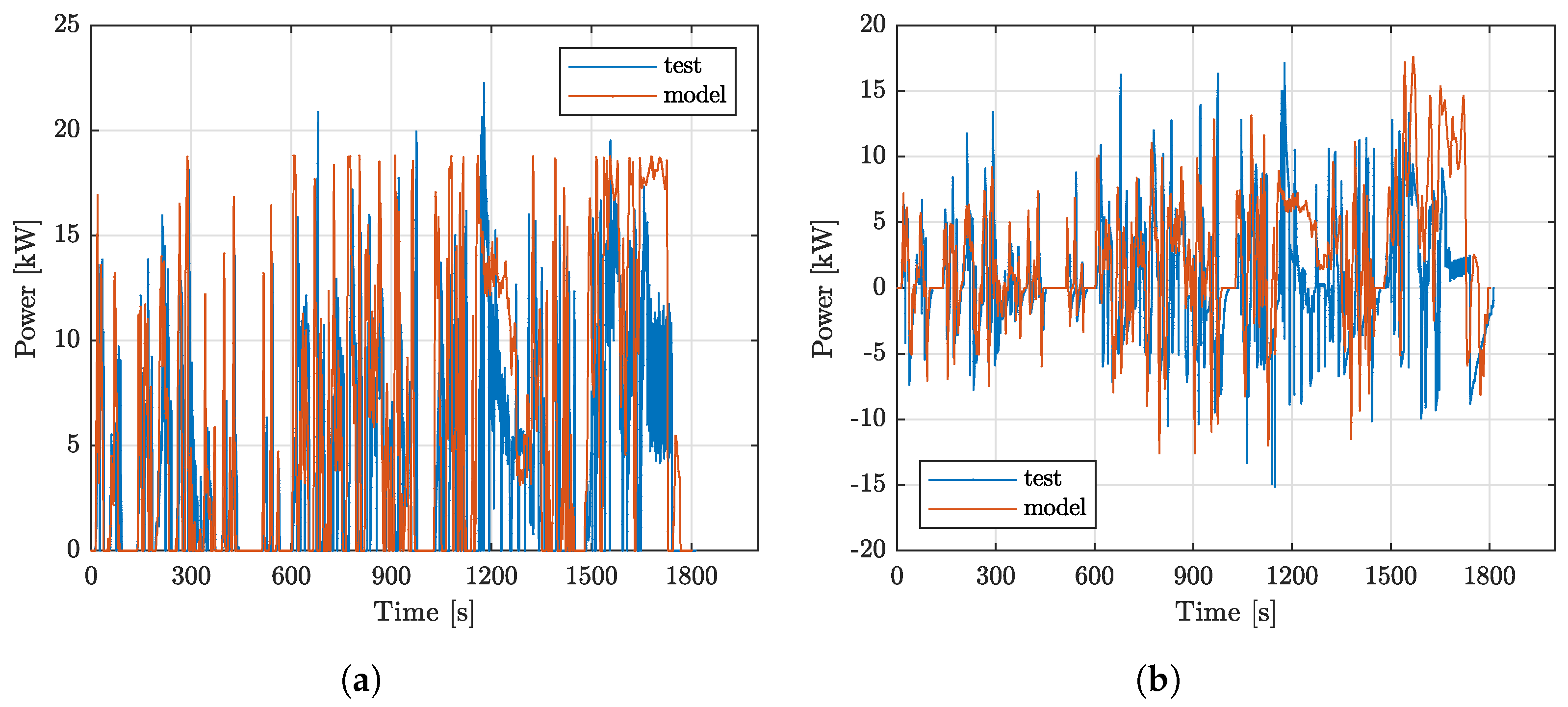
4.1. Model Validation

The model is validated with the independent calculation of all resistances that oppose the movement of the vehicle, resulting in the tractive force required to move the vehicle. These calculations are performed depending on the driving cycle analyzed and the characteristics that the vehicle will have both externally (body) and internally (powertrain).

To complete the validation, we compare the mechanical and electrical power obtained both with the simulation and with the development of the driving cycle on the chassis dynamometer. Figure 14a shows the electrical power of the model that is calculated second by second until the whole cycle is completed. There are small variations caused by different factors such as human error when performing the test, calibration error of the data acquisition tools, and environmental and surrounding factors. It should be emphasized that the model developed represents a highly efficient driver capable of performing the analyzed cycle perfectly.

Figure 14b shows the mechanical power obtained both in the model and the test in the chassis dynamometer. As mentioned, there are several factors that alter the similarity to 100% of both curves, but a similar trend is observed when the speed increases or decreases in the cycle.

4.2. Auxiliary Power Unit Integration

For using the ECMS, it is important to highlight that the revolutions at which the internal combustion engine rotates directly influence the energy produced and fuel consumption. Therefore, the objective is mainly to reduce fuel consumption and generate the greatest amount of energy, which in this case would become the equivalent energy that can be obtained with adequate control of the engine and the generator.

To meet this objective, and under the previous simulations, it is possible to observe that the revolutions in which the greatest amount of energy was obtained with the least consumption are between 1000 and 3500 rpm. For this, the state of charge is stabilized in a percentage initially established by the controller, and depending on the driving cycle, the control varies the revolutions of the engine and the generator depending on the SOC. To summarize, the SOC feeds the control, and the control sends the motor the revolutions at which it must work depending on the consumption and discharge of the batteries. A PID control is used to stabilize the SOC and control the engine with the necessary revolutions at which the generator will deliver the greatest energy depending on the requirement of the driving cycle; in this case, only the proportional (P) contains a saturation between 1000 and 3500 rpm.

Figure 15a shows the SOC and fuel consumption. In this specific case, the ICE generator operates at a constant 2300 rpm, and the fuel consumption line decreases linearly. Meanwhile, Figure 15b shows the trend that, in this case, fuel consumption is not linear, and the discharge trend is further controlled, unlike when it operates at a constant angular speed. In both cases, the driving cycle was analyzed. For WLTC-2, when the vehicle only developed one cycle, the APU is activated when the SOC reaches 45%. This analysis will also be carried out for the NEDC and WLTC-3 driving cycle, but it will be analyzed from when the SOC is at 100% and until the battery is completely discharged and reaches 0%.

4.3. Extra Weight Influence Due to the Integration of the APU in the EREV

When incorporating additional technology to extend the range of electric vehicles, such as an auxiliary power unit, the vehicle’s weight also increases. In this particular case, we consider the weight of the engine, which ranges from 90 kg to 160 kg. Additionally, the weight of a fully loaded fuel tank is 40 kg, resulting in an additional weight of 200 kg. Consequently, the total weight of the vehicle is 1570 kg, inclusive of the auxiliary power unit responsible for battery charging and completing the configuration of a series hybrid vehicle. Figure 16 shows the SOC comparison while running a WLTC-2 cycle, before and after adding the APU on the vehicle. It is seen that the increase in weight guarantees a faster depletion of the SOC.

When the auxiliary power unit is off (APU off mode), the vehicle will behave as a pure electric vehicle, where the battery will be discharged from 100% to 0%. Figure 17 shows the SOC behavior when running multiple cycles (NEDC, WLTC-2, WLTC-3, FTP75 and JC08), until a full battery depletion is reached. Different cycles guarantee diverse depletion rates, with the old standard NEDC, and the newer WLTC-2 and WLTC-3 being the cycles with the fastest depletion rate.

Table 3. Data collected, electric pure vehicle, NEDC, WLTC-2 and WLTC-3.

Driving Cycle	Energy [kWh]	Time [s]	Travel Dist. [km]
NEDC	39.70	34,065	315.57
WLTC-2	40.01	36,835	382.98
WLTC-3	33.99	21,341	306.78
FTP75	48.61	49,932	472.71
JC08	50.56	57,672	391.39

confirms these results, where the ratio between energy and depletion time is key. To the end of this study, the three aforementioned cycles with the fastest depletion rate were selected for experimental validation.

Nonetheless, the obtained results highlight a substantial difference in terms of depletion rate between the NEDC and the WLTC-3. The latter represents a more stressing duty cycle for the automobile and its subsystems, being the current standard for modern vehicle testing.

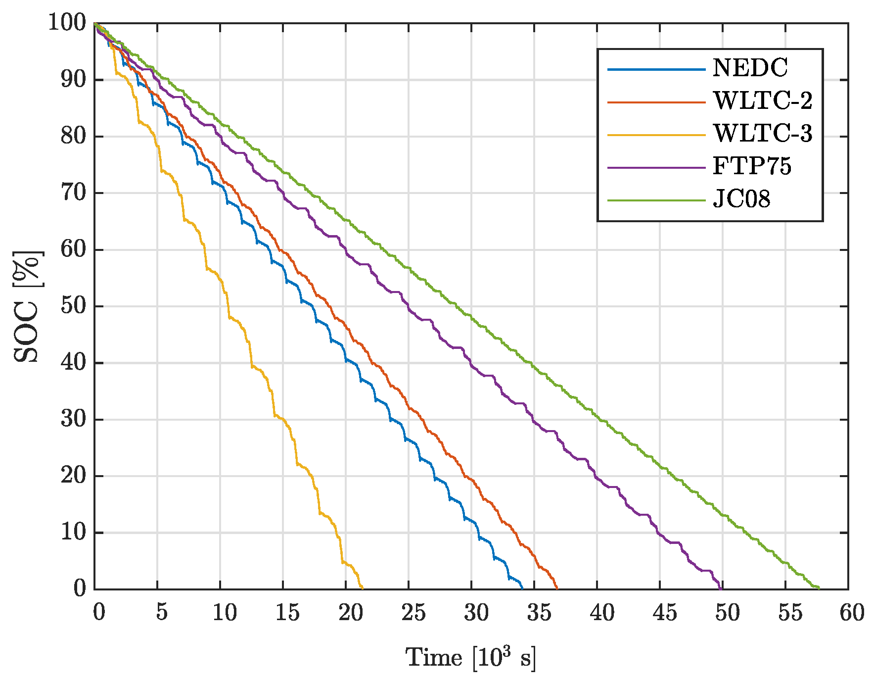
4.4. Analysis of SOC Behavior under Different APU Speeds

Figure 18 displays the state of charge (SOC) behavior of a battery over time during a cyclic New European Driving Cycle (NEDC) test. It shows how different speeds of an auxiliary power unit (APU) affect SOC depletion. In the following, the key points of this test set are outlined.

APU Activation: The APU is programmed to turn on when the SOC drops to a certain level (around 45%). This is indicated by a notable change in the slope of the SOC curve.

APU Deactivation: The APU continues to operate until the fuel is depleted as indicated by the points where the curves return to a steeper decline, marked as “APU Turn off”.

Different APU Speeds: The graph includes curves for various APU speeds (1200 rpm to 2300 rpm). Higher APU speeds generally result in a slower SOC decline when the APU is active, indicating more efficient charging or slower discharge due to better support from the APU.

SOC Depletion: The test continues until the battery reaches 0% SOC, showing the time taken to deplete the battery under different APU operation conditions. The overall pattern demonstrates how the intervention of the APU at different speeds impacts the battery’s discharge rate, offering insights into the efficiency and effectiveness of different APU settings in extending the vehicle’s range.

In the following section, the same analysis will be conducted for the WLTC-2 and WLTC-3 driving cycles. The focus will primarily be on the performance at 2300 rpm, where there is the highest energy generation. Additionally, the analysis will compare this fixed rpm approach with an active control strategy that automatically adjusts the rpm based on energy demand, forming the basis of the Equivalent Consumption Minimization Strategy. This comparison aims to evaluate the efficiency and effectiveness of these strategies in optimizing energy usage and battery longevity. A more detailed discussion is provided in the Section 5.

4.5. NEDC Analysis

Based on the generator characterization, the current and voltage recovered are low. Due to the generator’s low capacity, the energy produced is able to maintain the SOC between 40% and 45%. The generator is not able to charge the batteries, but with the delay, it extends the battery SOC until the fuel is totally consumed, and then the EREV becomes a pure electric vehicle again.

In this specific case, it is compared at the highest revolution at which the generator rotates, which is 2300 rpm, and compared to when the control is used; it can be seen in Figure 19.

To have a better perspective, the difference in the distance traveled is only 0.13% when comparing the maximum energy recovery capacity at 2300 rpm with the configuration where control is activated as shown in

Table 4. Comparison energy consumed, time and distance traveled and improvement, at APU off, constant speed and EMCS applied, and NEDC cycle.

Condition	Energy Cons. [kWh]	Travel Time [h]	Travel Dist. [km]	Improvement [%]
APU off	39.70	9.46	315.57	-
APU on/2300	48.19	12.73	424.49	34.52
APU on w/control	49.40	12.74	425.06	34.70

.

With the APU generator configuration, it is observed that when the vehicle operates solely as an electric vehicle and follows the NEDC driving cycle, it can travel 315.57 km. However, when the auxiliary power unit (APU) is activated in different modes, the percentage increase in distance traveled ranges from 2.76% to 34.51%. Furthermore, if the control strategy is activated, an increase of up to 34.69% is achieved.

4.6. WLTC-2 Analysis

When the vehicle develops the WLTC-2 vehicle speed profile according to the results shown in Figure 20, the blue and red lines represent the state of charge. When the SOC reaches 45%, the APU turns on and maintains the charge until it turns off; if we compare it between those ones, the blue line represents the battery SOC, and when the ICE generator turns at 2300 rpm, it tends to reach zero sooner. The same is true for fuel consumption; fuel tends to run out much sooner when the control strategy is not used.

Something important to comment on is that when the control strategy is used, the battery’s SOC is not stabilized at 45%; this is because the energy and revolutions at which the best efficiency is generated are not enough to stabilize the SOC. There is a 10% error, where the SOC is stabilized at around 40%.

The data from

Table 5. Comparison of energy consumed, time, and distance traveled and improvement at APU off, constant speed and EMCS applied, WLTC-2 cycle.

Condition	Energy Cons. [kWh]	Travel Time [h]	Travel Dist. [km]	Improvement [%]
APU off	40.01	10.23	382.98	-
APU on/2300	48.65	13.84	518.39	35.36
APU on w/control	50.34	14.25	533.42	39.28

indicate that, without the APU, the vehicle travels 382.98 km, consuming 40.01 kWh over 10.23 h. When the APU is activated at 2300 rpm, the distance traveled increases significantly to 518.39 km, representing an improvement of 35.36%, with energy consumption rising to 48.65 kWh and travel time extending to 13.84 h. With the APU control strategy activated, the distance further increases to 533.42 km, a 39.28% improvement over the baseline. This setup consumes 50.34 kWh over 14.25 h. The additional distance covered when using the APU at 2300 rpm compared to the baseline is 135.41 km, and the implementation of control adds another 15.03 km.

4.7. WLTC-3 Cycle Analysis

In the WLTC-3 cycle, it is where the most energy is demanded from the batteries at the moment of analysis when the ICE rotates at 2300 rpm; it can be seen in Figure 21 that a total of 28,548 s can be traveled according to the blue line that denotes the state of charge of the battery at these revolutions. At the same time, the red line that describes the SOC of the battery when using the control strategy can travel a total of 26,460 s, less than when used at constant revolutions. That is because the operating range for the control to work is between 1000 and 3500 rpm, but when the revolutions exceed these, the control is practically unable to find the most optimal range. That is why it can also not stabilize the SOC at 45%. In the same way, the behavior of fuel consumption with the control strategy is seen; it tends to be consumed and reaches zero earlier than when used at 2300 rpm. In the beginning, the consumption is delayed, but it tends to drop since the revolutions seek to stabilize the battery’s SOC but cannot due to the low power coming out of the generator.

Analyzing the distance that can be traveled according to the data obtained, when the control strategy is used, approximately 30 km less is traveled. Specifically, the distance when the vehicle is running purely electric is 306.78 km. However, when using the APU, the vehicle can extend its range significantly, offering up to a 33.74% increase in the total distance traveled, reaching 410.30 km as is shown in

Table 6. Comparison of energy consumed, time, and distance traveled and improvement at APU off, constant speed and EMCS applied, WLTC-3 cycle.

Condition	Energy Cons. [kWh]	Travel Time [h]	Travel Dist. [km]	Improvement [%]
APU off	37.60	5.93	306.78	-
APU on/2300	45.18	7.92	410.30	33.74
APU on w/control	44.22	7.35	380.21	23.94

. This increase is attributed to the ability of the APU to delay the depletion of the battery’s charge. Additionally, the use of the control strategy in this cycle allows the vehicle to cover 380.21 km, which is almost 10% less than the distance achieved when the engine runs at a constant 2300 rpm. This reduction occurs because the mechanical load and energy production vary with the control strategy, leading to more fuel consumption compared to maintaining a constant speed. Hence, while the control strategy provides benefits in fuel efficiency, it results in a slight decrease in the overall distance traveled compared to a fixed rpm setting.

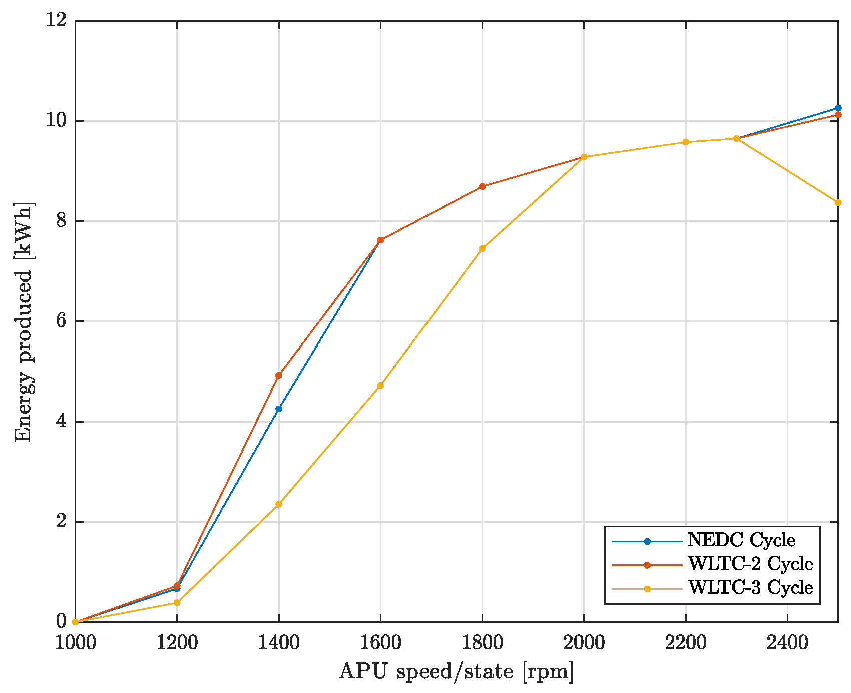
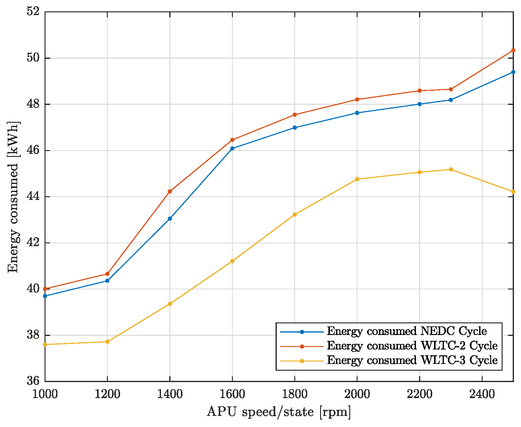
4.8. Equivalent Energy Produced ICE Generator

The analysis of energy output from the APU (ICE generator), powered by a 36 L gasoline tank, reveals notable differences across various driving cycles and rpm. The NEDC cycle shows a gradual increase in energy output from 0.67 kWh at 1200 rpm to a peak of 9.65 kWh at 2300 rpm without the control strategy. With the control strategy activated, the energy output further improves to 10.26 kWh, marking a 6.32% increase. This indicates that the control strategy can effectively optimize energy production, enhancing efficiency in less demanding cycles.

In the WLTC-2 cycle, a similar trend is observed. The energy output begins at 0.73 kWh at 1200 rpm and reaches a maximum of 9.65 kWh at 2300 rpm without control. The control strategy increases this output to 10.26 kWh, showing consistent improvement similar to the NEDC cycle. This consistent enhancement suggests that the control strategy is particularly beneficial in cycles with moderate energy demands.

However, in the WLTC-3 cycle, the control strategy’s effectiveness diminishes. Starting with an output of 0.39 kWh at 1200 rpm, the energy production increases but only reaches 8.37 kWh under the control strategy, compared to 9.65 kWh without it, resulting in a 13.26% deficit. This shortfall highlights the control strategy’s limitation in handling higher energy demands, likely due to increased mechanical load and fuel consumption variability.

Figure 22 illustrates the relationship between rpm and energy production, showing a clear increase in power generation as the rpm rises.

Table 7. Equivalent energy produced in NEDC, and WLTC-2 and WLTC-3 cycles by the 36 L tank, when the APU is off, the APU is on at a different constant speed, and the APU is on with the control active.

Speed or State [rpm]	Eq. Energy NEDC [kWh]	Eq. Energy WLTC-2 [kWh]	Eq. Energy WLTC-3 [kWh]
APU off	0	0	0
1200	0.67	0.73	0.39
1400	4.26	4.93	2.35
1600	7.62	7.62	4.73
1800	8.69	8.69	7.45
2000	9.28	9.28	9.28
2200	9.58	9.58	9.58
2300	9.65	9.65	9.65
APU on w/control	10.26	10.26	8.37

highlights the control strategy’s role in optimizing energy output, though its benefits are cycle dependent. The findings suggest that while control strategies can enhance efficiency, they must be finely tuned to the specific demands of each driving cycle to maximize effectiveness.

5. Discussion

One notable observation is the varying impact of the use of the ECMS strategy on different driving cycles and variable APU speeds, while considering the distance traveled (see Figure 23), and controlling the energy consumption (see Figure 24). This suggests that multiple factors, including the specific requirements of each driving cycle and the operational characteristics of the engine, influence the effectiveness of the control in optimizing vehicle performance. Moreover, the non-linear relationship between rpm, energy consumption, and distance traveled highlights the importance of implementing adaptive control strategies that can dynamically adjust engine operation to meet changing demands while minimizing energy wastage. Additionally, the significant improvements in both the energy efficiency and distance traveled achieved with the control engaged underscore the potential benefits of integrating advanced control systems into vehicle designs.

The data from the energy consumption

Table 8. Energy consumed comparison between the NEDC, WLTC-2 and WLTC-3 cycle, when the APU is off, the APU is on at a constant speed, and the APU is on with the control active.

Speed or State [rpm]	Energy Cons. NEDC [kWh]	Energy Cons. WLTC-2 [kWh]	Energy Cons. WLTC-3 [kWh]
APU off	39.7	40.01	37.6
1200	40.36	40.66	37.72
1400	43.05	44.23	39.36
1600	46.09	46.46	41.21
1800	46.99	47.55	43.23
2000	47.63	48.21	44.76
2200	48.01	48.59	45.06
2300	48.19	48.65	45.18
APU on w/control	49.4	50.34	44.22

, when compared to the distance traveled data provided by

Table 9. Distance traveled comparison between the NEDC, WLTC-2 and WLTC-3 cycle, when the APU is off, the APU is on at a constant speed and the APU is on with the control active.

Speed or State [rpm]	Travel Dist. NEDC [km]	Travel Dist. WLTC-2 [km]	Travel Dist. WLTC-3 [km]
APU off	315.57	382.98	306.78
1200	324.29	395.52	307.78
1400	360.1	463.95	332.27
1600	402.19	488.76	358.03
1800	413.63	504.01	384.84
2000	420.28	513.94	406.07
2200	424.21	518.12	409.93
2300	424.49	518.39	410.3
APU on w/control	425.06	533.42	380.21

, reveals key insights into the efficiency and performance of the vehicle across different driving cycles and APU states.

When the APU is off, the energy consumption for the NEDC, WLTC-2, and WLTC-3 cycles are 39.7 kWh, 40.01 kWh, and 37.6 kWh, respectively. Correspondingly, the distances traveled are 315.57 km, 382.98 km, and 306.78 km. With the APU activated at 2300 rpm, the energy consumption increases to 48.19 kWh (NEDC), 48.65 kWh (WLTC-2), and 45.18 kWh (WLTC-3). These energy increases correlate with significant increases in distance traveled to 424.49 km, 518.39 km, and 410.3 km, respectively.

The control strategy, while generally increasing energy consumption slightly, offers mixed results. For the NEDC and WLTC-2 cycles, energy consumption rises to 49.4 kWh and 50.34 kWh, with distances of 425.06 km and 533.42 km, respectively. This indicates an improvement in the distance despite higher energy usage, showing a more efficient utilization of energy. However, for the WLTC-3 cycle, the energy consumption under control is slightly lower at 44.22 kWh, but the distance traveled decreases to 380.21 km, compared to 410.3 km at a constant 2300 rpm without control.

This relationship highlights that while the control strategy can optimize energy efficiency and extend range in certain scenarios (as seen in NEDC and WLTC-2 cycles), it may not always provide benefits in more demanding conditions, such as the WLTC-3 cycle. The energy consumed versus distance traveled data demonstrates that the efficiency gains from the APU and control strategy depend heavily on the specific driving cycle and its demands. This is primarily due to the low power output of the APU, which limits its ability to meet the higher energy demands of certain cycles, particularly under more strenuous conditions like those presented in the WLTC-3 cycle.

The main contribution of this research lies in developing an algorithm and its associated methodology. This algorithm can provide a comprehensive energy analysis of an Extended-Range Electric Vehicle (EREV) and its behavior regarding the maximum distance it can travel. It delivers valuable information such as operating times, electrical power and energy generated and consumed, battery state of charge, and currents and voltages produced. Furthermore, this analysis is achieved without solely relying on equations, values, or efficiencies that represent the EREV under examination. The developed algorithm also allows the analysis of the powertrain behavior and how small changes in the vehicle’s overall structure can generate improvements and enhance efficiencies. And under that advantage of having the algorithm, a better differential transmission ratio was proposed that improves and increases the efficiency regarding energy consumption when the vehicle circulates under standardized driving cycles that are used worldwide. The algorithm can carry out different simulations, and depending on the inputs, comparisons can be made. The objectives can be fuel savings, emission reduction, and increasing the maximum distances that the vehicle can travel under standardized driving cycles. Analyzing the integration of a range extender module gives us a general and specific perspective of how a reasonable control, in this case, the ECMS, can increase the efficiency of using an APU that can operate at a constant speed. Of course, both criteria are valid depending on the objectives sought and remembering them, which can be to charge the batteries, maintain the state of charge or delay the discharge, depending on the power produced and delivered by the APU.

6. Conclusions

The APU configuration utilizing an ICE generator configuration, with a maximum power output of 3.2 kW, offers an improvement in additional distance ranging from 33.74% to 39% compared to pure electric operation. In both cases, power electronics play a crucial role in limiting current and voltage to avoid overloading the batteries. Consequently, if a higher-power generator is employed, the proportionality between the power output and improved distance remains consistent. It is important to note that these analyses are conducted using standardized cycles that allow for easy comparison with currently available vehicles, such as the Chevrolet Volt, which can achieve up to 675 km of autonomy with a full battery charge and fuel tank. The power capacity of the auxiliary power unit directly affects the maximum distance achievable with a full battery charge and full fuel tank, considering the internal configuration of the vehicle (battery type and capacity, engine type and characteristics, gearbox type and characteristics, vehicle type, and weight). This determines the applicability and benefits of integrating a range extender. The control strategy, guided by the PID control principle, aimed at stabilizing the state of charge (SOC) at a certain value, proves beneficial only when the power delivered by the APU configuration exceeds the energy consumption of the drive cycle. It is particularly effective when the batteries can be charged and not solely maintained at a specific state of charge. If the energy produced by the APU is less than the energy consumed by the drive cycle, the battery’s state of charge continuously depletes, resulting in minimal or no improvement, especially when using a high-power APU. When employing the ICE generator configuration, the energy generated and consumed throughout the standardized drive cycles demonstrates an improvement between 2.51% and 3.47%. As indicated by the results, in cases where the control strategy does not lead to improvement, it is optimal to operate the internal combustion engine (ICE) at a constant speed. This approach allows for the highest energy generation, considering the demand restrictions imposed by the specific composition of the drive cycle.

The adoption of tests in the old NEDC and the newer WLTC-2 and -3 cycles also highlight the demanding dynamic contributions induced by the latter in comparison to the other two. In this regard, the variability of the WLTC-3 profile may lead to a significant impact of parametric and dynamic uncertainties in the longitudinal model used to replicate the vehicle loads in a chassis dynamometer. Hence, further developments of this work will aim at validating the proposed strategy through road testing on a real vehicle.

References

1. Davis, S.C.; Boundy, R.G. Transportation Energy Data Book; US Department of Energy: Washington, DC, USA, 2022.
2. International Energy Agengy. Global EV Outlook 2023; Technical Report Geo; International Energy Agency: Paris, France, 2023. [Google Scholar]
3. Jin, Z.; Li, D.; Hao, D.; Zhang, Z.; Guo, L.; Wu, X.; Yuan, Y. Increasing the energy efficiency of an electric vehicle powered by hydrogen fuel cells. Int. J. Hydrogen Energy 2024, 49, 15326–15341. [Google Scholar] [CrossRef]
4. Zhang, Z.; Hao, D.; Wu, X.; Yuan, Y. PEM fuel cell as an auxiliary power unit for range-extended hybrid electric vehicles. Energy Convers. Manag. 2021, 256, 114765. [Google Scholar] [CrossRef]
5. Chen, J.; Wang, R.; Ding, R.; Luo, D. Matching design and numerical optimization of automotive thermoelectric generator system applied to range-extended electric vehicle. Appl. Energy 2024, 370, 123637. [Google Scholar] [CrossRef]
6. Jin, Z.; Li, D.; Hao, D.; Zhang, Z.; Wu, X.; Yuan, Y. A portable, auxiliary photovoltaic power system for electric vehicles based on a foldable scissors mechanism. Energy Built Environ. 2024, 5, 81–96. [Google Scholar] [CrossRef]
7. Zhang, Y.; Gao, B.; Jiang, J.; Liu, C.; Zhao, D.; Zhou, Q.; Chen, Z.; Lei, Z. Cooperative power management for range extended electric vehicle based on internet of vehicles. Energy 2023, 273, 127238. [Google Scholar] [CrossRef]
8. Boretti, A. High-efficiency internal combustion engine for hybrid hydrogen-electric locomotives. Int. J. Hydrogen Energy 2023, 48, 1596–1601. [Google Scholar] [CrossRef]
9. BMW i3. Available online: https://en.wikipedia.org/wiki/BMW_i3 (accessed on 1 August 2024).
10. Leach, F.; Kalghatgi, G.; Stone, R.; Miles, P. The scope for improving the efficiency and environmental impact of internal combustion engines. Transp. Eng. 2020, 1, 100005. [Google Scholar] [CrossRef]
11. Fan, L.; Tu, Z.; Chan, S.H. Prototype design of an extended range electric sightseeing bus with an air-cooled proton exchange membrane fuel cell stack based on a voltage control logic of hydrogen purging. J. Power Sources 2022, 537, 231541. [Google Scholar] [CrossRef]
12. Ouyang, T.; Zhao, Z.; Wang, Z.; Zhang, M.; Liu, B. A high-efficiency scheme for waste heat harvesting of solid oxide fuel cell integrated homogeneous charge compression ignition engine. Energy 2021, 229, 120720. [Google Scholar] [CrossRef]
13. Hahn, S.; Braun, J.; Kemmer, H.; Reuss, H.C. Optimization of the efficiency and degradation rate of an automotive fuel cell system. Int. J. Hydrogen Energy 2021, 46, 29459–29477. [Google Scholar] [CrossRef]
14. Zhou, Y.; Li, H.; Ravey, A.; Péra, M.C. An integrated predictive energy management for light-duty range-extended plug-in fuel cell electric vehicle. J. Power Sources 2020, 451, 227780. [Google Scholar] [CrossRef]
15. Hoeflinger, J.; Hofmann, P. Air mass flow and pressure optimisation of a PEM fuel cell range extender system. Int. J. Hydrogen Energy 2020, 45, 29246–29258. [Google Scholar] [CrossRef]
16. Toyota. Second Generation Toyota Mirai. Still Zero Emissions. Available online: https://www.toyota-europe.com/world-of-toyota/articles-news-events/2019/new-mirai-concept (accessed on 1 August 2024).
17. Hyundai NEXO de pila de Combustible | Hyundai | Hyundai Motor España. Available online: https://www.hyundai.com/es/modelos/nexo.html (accessed on 1 August 2024).
18. Nikola Two. Available online: https://nikolamotor.com/two (accessed on 1 August 2024).
19. Taner, T. The novel and innovative design with using H 2 fuel of PEM fuel cell: Efficiency of thermodynamic analyze. Fuel 2021, 302, 121109. [Google Scholar] [CrossRef]
20. Shen, X.; Costall, A.; Turner, M.; Islam, R.; Ribnishki, A.; Turner, J.; Vorraro, G.; Bailey, N.; Addy, S. Large-Eddy simulation of a Wankel rotary engine for range extender applications. In Powertrain Systems for Net-Zero Transport; Institution of Mechanical Engineers: Bath, UK, 2024; pp. 173–194. [Google Scholar] [CrossRef]
21. Ji, C.; Wang, H.; Shi, C.; Wang, S.; Yang, J. Multi-objective optimization of operating parameters for a gasoline Wankel rotary engine by hydrogen enrichment. Energy Convers. Manag. 2021, 229, 113732. [Google Scholar] [CrossRef]
22. Sadiq, G.A.; Al-Dadah, R.; Mahmoud, S. Development of rotary Wankel devices for hybrid automotive applications. Energy Convers. Manag. 2019, 202, 112159. [Google Scholar] [CrossRef]
23. Mazda 2 RE Range-Extender: Return of the Rotary—News—Car and Driver. Available online: https://www.caranddriver.com/news/a15366035/mazda-2-re-range-extender-return-of-the-rotary/ (accessed on 1 August 2024).
24. Zhao, J.; Ma, Y.; Zhang, Z.; Wang, S.; Wang, S. Optimization and matching for range-extenders of electric vehicles with artificial neural network and genetic algorithm. Energy Convers. Manag. 2019, 184, 709–725. [Google Scholar] [CrossRef]
25. Li, W.; Xu, H.; Liu, X.; Wang, Y.; Zhu, Y.; Lin, X.; Zhang, Y. Energy recovery control strategy for electric vehicles based on fuzzy neural network. Ain Shams Eng. J. 2024, 15, 102430. [Google Scholar] [CrossRef]
26. Dong, P.; Li, J.; Yao, K.; Li, S.; Wang, S.; Xu, X.; Guo, W. Downshifting strategy of plug-in hybrid vehicle during braking process for greater regenerative energy. Control Eng. Pract. 2024, 152, 106049. [Google Scholar] [CrossRef]
27. Wu, D.; Feng, L. On-Off Control of Range Extender in Extended-Range Electric Vehicle using Bird Swarm Intelligence. Electronics 2019, 8, 1223. [Google Scholar] [CrossRef]
28. Shah, R.M.R.A.; McGordon, A.; Rahman, M.M.; Amor-Segan, M.; Jennings, P. Characterisation of micro turbine generator as a range extender using an automotive drive cycle for series hybrid electric vehicle application. Appl. Therm. Eng. 2021, 184, 116302. [Google Scholar] [CrossRef]
29. Kim, H.; Nutakor, C.; Singh, S.; Jaatinen-Värri, A.; Nerg, J.; Pyrhönen, J.; Sopanen, J. Design process and simulations for the rotor system of a high-efficiency 22 kW micro-gas-turbine range extender for electric vehicles. Mech. Mach. Theory 2023, 183, 105230. [Google Scholar] [CrossRef]
30. Ezzat, M.F.; Dincer, I. Development and exergetic assessment of a new hybrid vehicle incorporating gas turbine as powering option. Energy 2019, 170, 112–119. [Google Scholar] [CrossRef]
31. Ji, F.; Zhang, X.; Du, F.; Ding, S.; Zhao, Y.; Xu, Z.; Wang, Y.; Zhou, Y. Experimental and numerical investigation on micro gas turbine as a range extender for electric vehicle. Appl. Therm. Eng. 2020, 173, 115236. [Google Scholar] [CrossRef]
32. Barakat, A.A.; Diab, J.H.; Badawi, N.S.; Bou Nader, W.S.; Mansour, C.J. Combined cycle gas turbine system optimization for extended range electric vehicles. Energy Convers. Manag. 2020, 226, 113538. [Google Scholar] [CrossRef]
33. Fathabadi, H. Utilizing solar and wind energy in plug-in hybrid electric vehicles. Energy Convers. Manag. 2018, 156, 317–328. [Google Scholar] [CrossRef]
34. Fathabadi, H. Recovering waste vibration energy of an automobile using shock absorbers included magnet moving-coil mechanism and adding to overall efficiency using wind turbine. Energy 2019, 189, 116274. [Google Scholar] [CrossRef]
35. Goushcha, O.; Felicissimo, R.; Danesh-Yazdi, A.H.; Andreopoulos, Y. Exploring harnessing wind power in moving reference frames with application to vehicles. Adv. Mech. Eng. 2019, 11, 168781401986568. [Google Scholar] [CrossRef]
36. Industrial Corporation Minuto de Dios Javier Roldán. Meet Eolo, A Wind-Powered EV From Colombia; Industrial Corporation Minuto de Dios Javier Roldán: Antioquia, Colombia, 2021. [Google Scholar]
37. Sun, B.; Li, B.; Xing, J.; Yu, X.; Xie, M.; Hu, Z. Analysis of the influence of electric flywheel and electromechanical flywheel on electric vehicle economy. Energy 2024, 295, 131069. [Google Scholar] [CrossRef]
38. Barelli, L.; Bidini, G.; Bonucci, F.; Castellini, L.; Fratini, A.; Gallorini, F.; Zuccari, A. Flywheel hybridization to improve battery life in energy storage systems coupled to RES plants. Energy 2019, 173, 937–950. [Google Scholar] [CrossRef]
39. Li, J.; Zhao, J. Energy recovery for hybrid hydraulic excavators: Flywheel-based solutions. Autom. Constr. 2021, 125, 103648. [Google Scholar] [CrossRef]
40. Erdemir, D.; Dincer, I. Assessment of Renewable Energy-Driven and Flywheel Integrated Fast-Charging Station for Electric Buses: A Case Study. J. Energy Storage 2020, 30, 101576. [Google Scholar] [CrossRef]
41. Wang, W.; Li, Y.; Shi, M.; Song, Y. Optimization and control of battery-flywheel compound energy storage system during an electric vehicle braking. Energy 2021, 226, 120404. [Google Scholar] [CrossRef]
42. Fan, T.; Liang, W.; Guo, W.; Feng, T.; Li, W. Life cycle assessment of electric vehicles’ lithium-ion batteries reused for energy storage. J. Energy Storage 2023, 71, 108126. [Google Scholar] [CrossRef]
43. Bou Nader, W.; Chamoun, J.; Dumand, C. Thermoacoustic engine as waste heat recovery system on extended range hybrid electric vehicles. Energy Convers. Manag. 2020, 215, 112912. [Google Scholar] [CrossRef]
44. Nader, W.B.; Chamoun, J.; Dumand, C. Optimization of the thermodynamic configurations of a thermoacoustic engine auxiliary power unit for range extended hybrid electric vehicles. Energy 2020, 195, 116952. [Google Scholar] [CrossRef]
45. Zhang, Z.; Zhang, X.; Chen, W.; Rasim, Y.; Salman, W.; Pan, H.; Yuan, Y.; Wang, C. A high-efficiency energy regenerative shock absorber using supercapacitors for renewable energy applications in range extended electric vehicle. Appl. Energy 2016, 178, 177–188. [Google Scholar] [CrossRef]
46. Kiddee, K.; Sukcharoensup, T. Efficiency Analysis of Suspension Energy Harvesting besed on Supercapacitor for Electric Vehicles. In Proceedings of the 2020 8th International Electrical Engineering Congress (iEECON), Chiang Mai, Thailand, 4–6 March 2020; pp. 1–4. [Google Scholar] [CrossRef]
47. Swamy, V.M.M.; Vidyasagar, S. High-efficiency regenerative shock absorbers considering twin ball screws transmission for increasing the vehicles’ driving range using a hybrid approach. Proc. Inst. Mech. Eng. Part I J. Syst. Control Eng. 2024, 238, 141–157. [Google Scholar] [CrossRef]
48. Siemens. Facts about Climate-Friendly Road Freight Transportation, Operational Range; Siemens: Munich, Germany, 2021; pp. 1–4. [Google Scholar]
49. Qiu, K.; Ribberink, H.; Entchev, E. Economic feasibility of electrified highways for heavy-duty electric trucks. Appl. Energy 2022, 326, 119935. [Google Scholar] [CrossRef]
50. Puma-Benavides, D.S.; Mixquititla-Casbis, L.; Llanes-Cedeño, E.A.; Jima-Matailo, J.C. Impact of Temperature Variations on Torque Capacity in Shrink-Fit Junctions of Water-Jacketed Permanent Magnet Synchronous Motors (PMSMs). World Electr. Veh. J. 2024, 15, 282. [Google Scholar] [CrossRef]
51. Puma-Benavides, D.S.; Izquierdo-Reyes, J.; Galluzzi, R.; Calderon-Najera, J.d.D. Influence of the final ratio on the consumption of an electric vehicle under conditions of standardized driving cycles. Appl. Sci. 2021, 11, 1474. [Google Scholar] [CrossRef]
52. Almousa, M.T.; Rezk, H.; Alahmer, A. Optimized Equivalent Consumption Minimization Strategy-based Artificial Hummingbird Algorithm for Electric Vehicles. Front. Energy Res. 2024, 12, 1344341. [Google Scholar] [CrossRef]
53. Du, A.; Chen, Y.; Zhang, D.; Han, Y. Multi-Objective Energy Management Strategy Based on PSO Optimization for Power-Split Hybrid Electric Vehicles. Energies 2021, 14, 2438. [Google Scholar] [CrossRef]
54. Yao, D.; Lu, X.; Chao, X.; Zhang, Y.; Shen, J.; Zeng, F.; Zhang, Z.; Wu, F. Adaptive Equivalent Fuel Consumption Minimization Based Energy Management Strategy for Extended-Range Electric Vehicle. Sustainability 2023, 15, 4607. [Google Scholar] [CrossRef]
55. Onori, S.; Serrao, L.; Rizzoni, G. Hybrid Electric Vehicles: Energy Management Strategies; Springer: London, UK, 2016; Volume 13. [Google Scholar]
56. Lei, Z.; Qin, D.; Hou, L.; Peng, J.; Liu, Y.; Chen, Z. An adaptive equivalent consumption minimization strategy for plug-in hybrid electric vehicles based on traffic information. Energy 2020, 190, 116409. [Google Scholar] [CrossRef]
57. Puma-Benavides, D.S.; Izquierdo-reyes, J.; Calderon-najera, J.D.D.; Ramirez-mendoza, R.A. A Systematic Review of Technologies, Control Methods, and Optimization for Extended-Range Electric Vehicles. Appl. Sci. 2021, 11, 7095. [Google Scholar] [CrossRef]
58. Zhang, J.; Wang, Z.; Liu, P.; Zhang, Z.; Li, X.; Qu, C. Driving cycles construction for electric vehicles considering road environment: A case study in Beijing. Appl. Energy 2019, 253, 113514. [Google Scholar] [CrossRef]
59. Yang, H.; Wu, J.; Chen, F.; Guo, Z.; Xue, X.; Chen, Y.; Xu, G. Life cycle climate performance evaluation of electric vehicle thermal management system under Chinese climate and driving condition. Appl. Therm. Eng. 2023, 228, 120460. [Google Scholar] [CrossRef]
60. Wu, A.; Zhang, Z.; Shi, X.; Liu, C. Modeling the role of interfacial adhesion in the rolling resistance of a hyperelastic wheel. Tribol. Int. 2023, 185, 108494. [Google Scholar] [CrossRef]
61. Chen, Z.; Liu, Y.; Ye, M.; Zhang, Y.; Li, G. A survey on key techniques and development perspectives of equivalent consumption minimisation strategy for hybrid electric vehicles. Renew. Sustain. Energy Rev. 2021, 151, 111607. [Google Scholar] [CrossRef]
62. Anselma, P.G.; Biswas, A.; Belingardi, G.; Emadi, A. Rapid assessment of the fuel economy capability of parallel and series-parallel hybrid electric vehicles. Appl. Energy 2020, 275, 115319. [Google Scholar] [CrossRef]
63. Zhuotong, L.; Yi, Z.; Yun, J.; Fang, F. Rule-Based Dual Planning Strategy of Hybrid Battery Energy Storage System. IFAC-PapersOnLine 2022, 55, 495–500. [Google Scholar] [CrossRef]
64. ISO 28580; Passenger Car, Truck and Bus Tyre Rolling Resistance Measurement Method—Single Point Test and Correlation of Measurement Results. International Organization for Standardization: Geneva, Switzerland, 2018.
65. Puma-Benavides, D.S.; Cevallos-Carvajal, A.S.; Masaquiza-Yanzapanta, A.G.; Quinga-Morales, M.I.; Moreno-Pallares, R.R.; Usca-Gomez, H.G.; Murillo, F.A. Comparative Analysis of Energy Consumption between Electric Vehicles and Combustion Engine Vehicles in High-Altitude Urban Traffic. World Electr. Veh. J. 2024, 15, 355. [Google Scholar] [CrossRef]
66. Cabir, B.; Yakin, A. Evaluation of gasoline-phthalocyanines fuel blends in terms of engine performance and emissions in gasoline engines. J. Energy Inst. 2024, 112, 101483. [Google Scholar] [CrossRef]
Figure 1. Analyzed configuration of an Extended-Range Electric Vehicle.
Wevj 15 00439 g001
Figure 2. Energy flow modes. (a) Discharge mode: only the battery delivers the power. (b) Charge mode: the generator charges the battery. (c) Stable mode: the generator delivers the power to the electric motor, and the battery maintains the SOC.
Wevj 15 00439 g002
Figure 3. Improved compact ICE–Extended-Range EV–powertrain module methodology.
Wevj 15 00439 g003
Figure 4. Algorithm usage scenarios.
Wevj 15 00439 g004
Figure 5. Experimental setup scheme (left) and picture (right). (1) Engine Z16SE, (2) engine dynamometer SUPERFLOW SF902, (3) air intake, (4) gas analyzer, (5) ECU, (6) ignition coil, (7) exhaust, (8) gas analysis probe, (9) fuel tank, (10) fuel pump, (11) generator/alternator, (12) Fluke 43b power analyzer. Yellow line: ignition current. Red line: fuel supply and measurement. Blue line: control. Green line: alternator current measurement.
Wevj 15 00439 g005
Figure 6. Process diagram of the operation of the control strategy.
Wevj 15 00439 g006
Figure 7. Power and torque measured on the dynamometer chassis.
Wevj 15 00439 g007
Figure 8. Longitudinal model of the vehicle. Reprinted from [51].
Wevj 15 00439 g008
Figure 9. Characteristic curves torque and power engine Z16SE.
Wevj 15 00439 g009
Figure 10. Specific fuel and theoretical maximum fuel consumption curves Z16E Engine. (a) Specific fuel consumption; (b) theoretical maximum fuel consumption.
Wevj 15 00439 g010
Figure 11. Generator characteristic curves. (a) Generator characteristic curve of voltage; (b) generator characteristic curve of current.
Wevj 15 00439 g011
Figure 12. Mechanical load and rpm variation on stable mode and charge mode.
Wevj 15 00439 g012
Figure 13. Extended-Range Electric Vehicle diagram. Adapted from [51].
Wevj 15 00439 g013
Figure 14. Power characteristics of the generator. (a) Electric power model and test in WLTC-3 cycle; (b) mechanical power WLTC-3 cycle.
Wevj 15 00439 g014
Figure 15. Battery SOC and fuel consumption for ICE@2300 rpm and with control. (a) SOC and fuel consumption ICE@2300 rpm per cycle; (b) SOC and fuel consumption with control per cycle.
Wevj 15 00439 g015
Figure 16. Comparison of the SOC between EV mode, blue line, versus EREV mode (APU included), the orange line.
Wevj 15 00439 g016
Figure 17. SOC behavior NEDC, WLTC-2 and WLTC-3, discharge mode, APU off, electric pure vehicle.
Wevj 15 00439 g017
Figure 18. SOC behavior at different ICE speeds NEDC.
Wevj 15 00439 g018
Figure 19. Comparison of SOC and fuel consumption, at a constant speed and EMCS applied, and NEDC cycle.
Wevj 15 00439 g019
Figure 20. Comparison of SOC and fuel consumption at a constant speed and EMCS applied, WLTC-2 cycle.
Wevj 15 00439 g020
Figure 21. Comparison of SOC and fuel consumption, at a constant speed and EMCS applied, WLTC-3 cycle.
Wevj 15 00439 g021
Figure 22. Equivalent energy produced by the 36 L tank on the WLTC-3, WLTC-2 and NEDC cycles; comparison of the energy produced by the APU (ICE generator).
Wevj 15 00439 g022
Figure 23. Distance traveled on NEDC, WLTC-2, and WLTC-3.
Wevj 15 00439 g023
Figure 24. Energy produced and consumed on NEDC, WLTC-2, and WLTC-3.
Wevj 15 00439 g024