Abstract
This analysis compares the energy efficiency and operational costs of combustion vehicles (Hyundai Accent 1.6 L and Chevrolet Sail 1.5 L) with the Nissan Leaf, an electric vehicle, under current fuel and electricity pricing in Ecuador. Combustion vehicles, converting gasoline into mechanical energy, demonstrate substantial energy losses, leading to higher operational costs, especially with recent gasoline price hikes to USD 2.722 per gallon. In stark contrast, the Nissan Leaf exhibits significantly greater energy efficiency, consuming only 15–20 kWh per 100 km, which translates to lower running costs (USD 11.20 to fully charge a 40 kWh battery). Despite the clear economic and environmental benefits of electric vehicles, their adoption in Ecuador is hampered by geographical challenges such as diverse terrain that can affect vehicle range and battery longevity. Moreover, the limited and uneven distribution of EV charging stations, mostly concentrated in urban areas, poses significant barriers. For broader implementation, a strategic expansion of the EV infrastructure and careful consideration of the national energy grid’s capacity to support increased electric vehicle uptake are essential. Addressing these challenges is crucial for realizing the full potential of electric vehicles in enhancing Ecuador’s sustainability and energy independence.
1. Introduction
The evolution of the automotive industry has led to significant advancements in vehicular technologies aimed at enhancing energy efficiency and reducing environmental impact. Increasing vehicle efficiency and lowering emissions are pivotal in combating climate change and urban air pollution, challenges that are particularly pressing in densely populated and high-altitude areas. The transportation sector is a major contributor to global greenhouse gas emissions, primarily due to the extensive use of fossil fuels in traditional internal combustion engine vehicles [1].
In response to these environmental challenges, there has been a shift towards developing and deploying more efficient vehicle technologies, including hybrid, electric, and alternative fuel vehicles [2]. These technologies not only promise reduced greenhouse gas emissions but also offer improvements in energy consumption per distance traveled [3]. Electric vehicles (EVs), for instance, utilize energy more efficiently than conventional gasoline vehicles, converting over 60% of the electrical energy from the grid to power at the wheels, compared to about 20% for gasoline vehicles [4].
Furthermore, the implementation of variable driving conditions, such as those involving variable slopes, imposes additional demands on vehicle performance and efficiency [5,6]. High-altitude regions, such as Riobamba, pose unique challenges due to thinner air and potential reductions in engine combustion efficiency and battery performance. These conditions necessitate a deeper investigation into how different vehicle types perform under such environmental stresses.
This study initially focused on the fuel consumption of gasoline vehicles navigating through high-altitude, variable-slope conditions in Riobamba, where the changing engine loads significantly impact fuel consumption and emissions [7]. Recognizing the critical need for sustainable transportation solutions, this research aims to examine the viability and performance of electric vehicles under identical route conditions, providing a direct comparison of energy efficiency and environmental impacts between gasoline-powered and electric vehicles [8].
Ecuador’s commitment to renewable energy sources significantly enhances the feasibility and environmental benefits of electric vehicle (EV) adoption. With 92% of its electricity generated from hydroelectric sources, complemented by investments in wind, solar, and other non-conventional renewables [9]. EVs in Ecuador would primarily be powered by clean energy, drastically reducing the carbon footprint compared to traditional vehicles. These data underscore Ecuador’s heavy dependence on hydroelectric power, with limited diversification into other renewable energy sources. Ongoing projects like the Villonaco II and III wind farms and the El Aromo solar plant, alongside government policies fostering private investment and energy efficiency, underscore a robust framework for sustainable transportation [10]. The deployment of EVs, supported by renewable energy, aligns with national efforts to mitigate climate change, promote economic growth through job creation, and reduce dependency on fossil fuels, particularly in sensitive areas like the Galápagos.
Ecuador’s COMEX Resolution 016-2019 establishes a policy to promote the use of electric vehicles by exempting them from tariffs and taxes [11]. This resolution eliminates import duties and taxes on electric vehicles and their sales, making electric vehicles more affordable for consumers. The goal is to reduce the financial barriers associated with purchasing electric vehicles, thereby encouraging more people to opt for environmentally friendly transportation options.
By removing these financial obstacles, the resolution fosters the adoption and use of electric vehicles in Ecuador. It supports the government’s broader environmental and energy efficiency goals by facilitating a shift towards cleaner transportation. The increased affordability of electric vehicles is expected to drive higher sales, contributing to reduced greenhouse gas emissions and reliance on fossil fuels.
1.1. Objectives
The primary aim of this research is to thoroughly evaluate and compare the energy efficiency of gasoline and electric vehicles under identical driving conditions, focusing on a specific driving cycle. This involves several detailed objectives aligned with a singular scope to ensure a focused and comprehensive analysis:
- Evaluate the Fuel Consumption of Gasoline Vehicles: Conduct an in-depth analysis of fuel consumption for the gasoline vehicles previously studied, focusing on the specific driving cycle used. This includes examining how the vehicles’ performance is influenced by variable slopes and high-altitude conditions, which are characteristic of the route in the original study.
- Simulate Energy Consumption for an Electric Vehicle: Develop a simulation of an electric vehicle following the same driving cycle used by the gasoline vehicles. The simulation will aim to replicate the vehicle dynamics and environmental conditions to accurately compare its performance against that of the gasoline vehicles.
- Compare Energy Efficiency: Compare the energy consumption data from the gasoline vehicles with the simulated data from the electric vehicle. This comparison will focus on the energy efficiency of each vehicle type per 100 km traveled under the same driving conditions. It will include metrics such as energy or fuel consumed, distance covered, and the influence of route topography and vehicle dynamics.
1.2. Significance
The comparative analysis between gasoline and electric vehicles under specified conditions will provide valuable insights into the potential of electric vehicles to replace traditional gasoline vehicles in specific geographic and traffic scenarios.
At high altitudes, both combustion engines and electric vehicles face unique challenges that significantly impact their performance and efficiency.
On the ICE vehicles, the reduced oxygen levels at high altitudes affect the combustion process in internal combustion engines, leading to incomplete combustion and higher fuel consumption. This results in decreased engine efficiency, with studies showing that fuel economy can decrease by up to 20% in high-altitude conditions compared to sea level. The primary factors influencing these changes are the lower atmospheric pressure and reduced oxygen concentration, which cause variations in emissions such as increased carbon dioxide (CO2), carbon monoxide (CO), and nitrogen oxides (NOx) at higher altitudes [12].
Electric vehicles (EVs), on the other hand, are less affected by changes in air density but still face significant challenges in high-altitude environments. The increased load from climbing slopes typical of mountainous terrain results in higher energy consumption. Although regenerative braking can help recover some energy during descents, it does not fully offset the increased consumption from ascending inclines. Consequently, the overall energy consumption of EVs is higher in hilly or mountainous regions compared to flat, low-altitude areas [13].
Analyzing the impact of high altitude on both combustion engines and electric vehicles is crucial for developing tailored strategies to manage fuel and energy efficiency under these conditions. Understanding the specific challenges each type of vehicle faces allows for a better optimization of performance and more accurate planning for fuel and energy requirements in high-altitude regions. This comparative analysis is essential for improving the reliability and efficiency of transportation in diverse environmental conditions, ensuring that both types of vehicles can operate effectively in various terrains.
This study will contribute to the broader understanding of transportations’ environmental impacts, informing policy decisions and public transport strategies in regions similar to Riobamba. Moreover, the findings could support initiatives aimed at promoting electric vehicles as a viable alternative in high-altitude cities, aligning with global trends towards sustainable mobility solutions.
2. Methodology
The methodology described in Figure 1 is divided into four main phases: definition; test route; vehicle model development; and comparison, analysis, and results. In the definition phase, the base study vehicles are defined, the route is described, and the tools and scope of the study are determined. The test route phase includes on-board diagnostics and fuel consumption tests for data collection. In the vehicle model development phase, conceptual analysis is carried out, dynamic equations are established, and simulation tools are used. Finally, in the comparison, analysis, and results phase, energy efficiency is calculated, efficiencies are compared, and the conclusions and results obtained are discussed. The methodology used is intended to show the impact of combustion vehicles on fuel consumption and the feasibility of using electric vehicles in the same routes and the respective comparative.
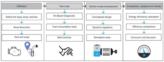
Figure 1.
Methodology used to compare the energy efficiency between electric vehicle simulated and combustion vehicles tested.
2.1. Vehicle Selection
For the experimental research, three types of vehicles will be used, two gasoline-powered and one electric-powered vehicle, whose technical characteristics are detailed in Table 1. Combustion vehicles were selected, according to the statistics of the Mobility Plan of the Riobamba Canton. As the most used by the inhabitants of the province and for the selection of the electric vehicle, it was considered that it has similar characteristics to the internal combustion vehicles selected. The Nissan Leaf is chosen as the representative EV model due to its popularity and extensive data availability. It is one of the most widely used electric vehicles globally, making it a relevant and practical choice for comparative studies. Its performance characteristics, such as battery capacity, energy efficiency, and regenerative braking capabilities, are well documented, providing a reliable basis for simulation and analysis.

Table 1.
Principal characteristics of the vehicles.
2.2. Route Description
The province of Chimborazo, where Riobamba is located, has a population of approximately 264,048 people as of 2024. Riobamba, the capital city, is a significant regional center with around 150,000 inhabitants. The city is notable for its historical significance and its role as a transport hub in the central Andes.
The route is located between Riobamba and Guano cantons (see Figure 2). The route has been selected due to the large vehicular influx that exists in these cantons that will help us to determine the fuel consumption in real traffic conditions in the Chimborazo province [14,15]. This route will cover 21.8 km (21,800 m) that will be divided into one 7 km (7000 m) suburban route and a 14.8 km (14,800 m) urban route. There is an altitude variation from 2715 to 2876 m above sea level (Figure 3).

Figure 2.
Chimborazo province peripheral route.
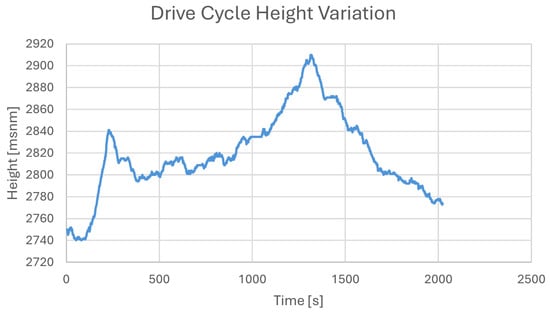
Figure 3.
Height variation drive cycle analyzed; Chimborazo–Ecuador route.
Figure 4 shows the driving cycle of the route; it presents a time series of vehicle speeds over approximately 2500 s. Here are some key observations:
- Variability: The speed is highly variable, reflecting typical real-world driving conditions where speeds fluctuate due to traffic, road conditions, or driver behavior. The speed oscillates frequently between as low as approximately 0 m/s and as high as approximately 25 m/s.
- High-Speed Phases: There are several distinct phases where the speed peaks notably. For example, around 300–400 s, 800–900 s, and 1800–1900 s, the speed reaches near the maximum. These could represent highway driving or overtaking scenarios.
- Low-Speed or Idle Phases: There are periods where the speed drops to near 0 m/s, such as around 1200 s and 2200 s. These could indicate stopping conditions, perhaps at traffic signals or due to congestion.

Figure 4.
Speed variation drive cycle analyzed; Chimborazo–Ecuador route.
Figure 4.
Speed variation drive cycle analyzed; Chimborazo–Ecuador route.

2.3. Data Collection
Two methods of collecting information, OBD II System and External Fuel Tank, are used to ensure the accuracy and reliability of the fuel consumption data.
2.3.1. The External Fuel Tank (Canister)
The External Fuel Tank method involved using a Liqui Moly brand pressurized canister with a 5L capacity to measure fuel consumption directly and precisely. This setup required securely installing the canister in the vehicle, ensuring it supplied fuel to the engine, and pressurizing it to 80 PSI for consistent fuel flow. Initial and final fuel volumes were recorded to determine the exact amount of fuel consumed during the test. This method was applied to both the Hyundai Accent 1.6L and Chevrolet Sail 1.5L vehicles.
The external fuel tank is securely installed in the vehicle, ensuring that it is properly connected to the fuel supply system. This setup involves integrating the canister in a way that it directly supplies fuel to the engine, bypassing the vehicle’s internal fuel tank. The canister is pressurized to a specific level, up to 80 PSI, as per the manufacturer’s specifications. This pressurization ensures a consistent and controlled fuel flow to the engine, mimicking normal operating conditions [16].
2.3.2. Onboard Diagnosis System OBDII
The ELM327 device allows for the acquisition of multiple information with considerable precision, thus allowing for the determination of fuel consumption in addition to different variables that objectively describe a driving pattern based on the engine control unit (ECU), in which variables (speed, time, engine, revolutions, etc.) can be obtained from the different sensors that are incorporated into the vehicles from the diagnostic port onboard (OBD) [17,18]. The system is in charge of fully monitoring and controlling the engine. The precision of the data that are obtained from the fuel consumption using the interface of the OBD port will be validated with the external tank. Figure 5 shows the sequence of the data gathering, starting from the engine connected at the OBD port to obtain fuel consumption data.

Figure 5.
On-board diagnostic function chart.
2.4. Fuel Description
The fuels used in the tests were Extra and Ecopaís, both of which have 85% octane. Extra is a regular gasoline widely available and used in public transport due to its affordable cost. It is composed of pure gasoline without additional additives, making it an economical but less efficient option in terms of energy performance and emissions. Ecopaís, on the other hand, is gasoline that contains 5% ethanol, a biofuel derived from renewable sources [19,20]. This additive improves engine combustion, resulting in better fuel performance and lower pollutant emissions. Additionally, Ecopaís is part of a government initiative to reduce dependence on fossil fuels and decrease the environmental impact of transportation.
2.5. Fuel Vehicle Test
Before the tests, the vehicles were subjected to a mechanical and electronic review of their condition. A preventive maintenance was carried out to guarantee the perfect condition of the systems.
The next points describe the protocol used before the tests. The control of the initial parameters are the same in all tests:
- Verify the environmental conditions;
- Check that the tire pressure is at the manufacturer’s recommended level;
- Install and secure the equipment for the measurement of fuel consumption and revolution control;
- Start the vehicle and warm up the engine until it reaches the normal operating temperature that corresponds to 95 °C;
- Check that the vehicle accessories are deactivated;
- Verify the correct operation equipment;
- Start in the selected route;
- Record the obtained data;
- Repeat the process for each test with normal driving.
2.6. Experimental Design
For the tests, two methods are used to obtain fuel consumption data: the OBD II System (ELM327) and the External Fuel Tank (Canister). Four tests were conducted for each vehicle using both Extra and Ecopaís fuels. A total of 4 tests of each type of fuel was carried out to determine significant differences between the experimental groups. For this study, the dependent variables’ behavior is presented when using the two types of fuel in the two test vehicles with different cylinder capacities: instantaneous consumption (km/L) and long performance consumption (L/100 km). For the statistical study of the results, the nomenclature presented in Table 2 is taken.
Table 2.
Experimental factors and levels, nomenclature, and array.
2.7. Electric Vehicle Simulation
This section outlines the mathematical models employed to depict vehicle dynamics and battery performance. The simulation depends on the characteristics of the 40 kW Nissan Leaf vehicle [21].
2.8. Vehicle Dynamics
The vehicle’s longitudinal dynamics consider only throttle and brake control actions, while vertical, lateral, and roll dynamics are disregarded. The forward motion of the car must counteract the following forces:
- Rolling resistance;
- Aerodynamic drag;
- The effect of vehicle weight on inclined roads;
- Inertial forces during changes in velocity.
This scenario is illustrated in the free-body diagram shown in Figure 6.
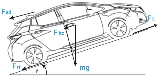
Figure 6.
The forces exerted on the electric vehicle while ascending a slope.
2.8.1. Rolling Resistance Force
This force arises from the friction between the vehicle’s tires and the road surface. It can be described as
where is the rolling resistance coefficient using a value of 0.014984 to represent it, m denotes the vehicle’s mass, and is the acceleration due to gravity.
2.8.2. Aerodynamic Drag
This force results from the resistance encountered by the vehicle’s body as it moves through the air. It is expressed as
where represents the air density in Riobamba due to the city’s altitude, is the aerodynamic drag coefficient, A denotes the vehicle’s frontal area, and v is its longitudinal speed. In this case, was determined using computational fluid dynamics (CFD) simulations and has a value of 0.28, whereas A was measured based on the vehicle’s dimensions, resulting in a value of 2.27 m2.
2.8.3. Hill Climbing Force
This term represents the force required to propel the vehicle uphill on an inclined road:
where represents the angle of the road incline.
Figure 7 displays variations in the slope on route used on this research, over approximately 2000 s. These data are significant because it represents the impact of terrain on driving, which is crucial for understanding how an electric vehicle like the Nissan Leaf performs under varied geographical conditions.
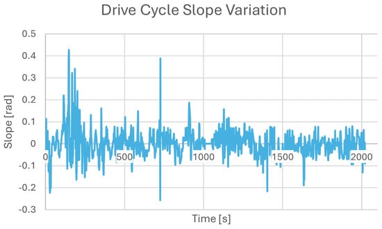
Figure 7.
Slope variation drive cycle analyzed; Chimborazo–Ecuador route.
The slope reveals a range of slope values from about −0.3 to 0.5 radians, where positive values indicate uphill and negative values indicate downhill scenarios. Notably, there is a significant spike to nearly 0.5 radians around the 200 s mark, suggesting a steep uphill drive that tests the vehicle’s performance on sudden inclines. Additionally, the slope values fluctuate throughout, with periods of rolling terrain where the vehicle experiences alternating ascents and descents, as well as stable phases of slight positive or negative slopes, simulating more gentle and consistent terrain changes.
2.8.4. Net Force
The vehicle’s acceleration can be calculated using Newton’s second law by first determining the net thrust as a function of speed. It is important to note that the vehicle’s translational motion is linked to the rotational motion of the components connected to the wheels, such as the engine and driveline. Consequently, any change in translational speed will correspond to a change in the rotational speed of these components. To account for this, the mass factor is introduced in the following equation to determine the vehicle’s acceleration a [22]. This factor considers the impact of the inertia of the rotating parts on the vehicle’s acceleration characteristics. The resulting equation is
The mass factor is determined by the moments of inertia of the rotating components, such as the wheels, gearbox gears, and differential. For instance, in passenger cars, the mass factor can be calculated using the following formula:
The first term on the right-hand side of Equation (5) accounts for the contribution of the rotational inertia of the wheels. In contrast, the second term represents the contribution of the inertia from the components rotating at the equivalent engine speed, factoring in the overall gear reduction. Here, refers to the gearbox ratio, while represents the differential or final drive ratio.
2.8.5. Tractive Force
The tractive force is determined by summing up the contributions of the previously mentioned forces:
As a result, the tractive force is converted into power using the following method.
2.8.6. Gradability
Gradability is typically defined as the steepest incline a vehicle can ascend at a constant speed. On a slope, the tractive effort must counteract grade resistance, rolling resistance, and aerodynamic drag. For a relatively small incline angle, , . Therefore, by solving for from Equation (3), we obtain
where represents the maximum incline the vehicle can handle, denotes the engine power, and indicates the efficiency of the drivetrain.
2.9. Battery Model
The battery, a lithium-ion cell pack, is characterized by its state of charge , which measures its energy level. indicates a fully charged battery, while an , signifies a fully depleted battery. The energy flowing into the battery (charge, ) or out of the battery (discharge, ) is calculated at each time step during driving, as follows:
In these equations, t represents time, is the nominal voltage, K is the polarization constant, i is the battery current, is the current filtered with a low-pass filter (), Q denotes the maximum battery capacity, is the exponential voltage, and is the exponential capacity.
For the battery simulation, Table 3 shows the characteristics of a Nissan leaf battery of 40 kWh.
Table 3.
Nissan Leaf 40 kWh battery characteristics.
2.10. Simulations
A numerical model can be used to calculate the power needed for traction as the vehicle moves along the road. This traction power is directly related to the force generated by the electric motor. The following assumptions are made for the vehicle model calculations:
- The vehicle moves exclusively in the longitudinal direction.
- The system is assumed to be ideally rigid, with no consideration of vibration or damping effects.
- The tire radius is considered constant.
A backward vehicle model was developed and tested using MATLAB/Simulink® R2022b. Figure 8 illustrates the general block diagram of the model, beginning with the speed profile provided by the driving cycle, which leads to the block where the required mechanical power is calculated. The model is further enhanced by computing the major opposing forces to the vehicle’s movement and converting these values through the gearbox ratios and the differential. The next step involves converting electrical energy to mechanical energy in the electric motor, with the motor’s efficiency taken into account. The induction machine then requires varying current profiles based on the traction demand in the electrical domain. Energy consumption is determined by solving all the equations with respect to time, which corresponds to the duration needed to complete the driving cycle.
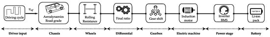
Figure 8.
Block diagram illustrating the operation of the backward dynamic model for an electric vehicle in MATLAB/Simulink®. Reprinted from Ref. [21].
In this context, employing a backward model operates under the assumption that the vehicle can accurately replicate all the speed points from the input profile. This assumption is particularly valid when simulating standardized driving cycles, as was performed in this case. One advantage of this approach is that it requires significantly fewer resources compared to forward models [23].
The simulations assume the vehicle weight includes a person onboard weighing approximately 80 kg, with an ambient temperature set at 22 °C. The electric motor’s efficiency is modeled to range between 86% and 94%, varying with operating speed, and the battery starts at a full charge (100% SOC) at the beginning of the simulations. Factors affecting accuracy include simplifications in models, which assume ideal conditions such as constant tire radius, no vibrations, and perfect efficiency in components. Environmental variability, such as road surface irregularities and driver behavior, introduces variability that simulations struggle to fully capture. Additionally, discrepancies arise from differences in the precision of tools used for data acquisition in real measurements compared to theoretical calculations in simulations.
The model was validated by the Automotive Mechatronics Research Center (CIMA) using an electric vehicle through standardized driving cycles of the New European Driving Cycle (NEDC), Worldwide Harmonized Light Vehicles Test Cycle (WLTC-2), and WLTC-3. These results indicate that the simulation model is relatively accurate, with discrepancies ranging from −2.39% to +11.77% compared to real measurements [21].
2.11. Driving Cycles
Driving cycles consist of a series of variable longitudinal velocity set points over time. In the context of electric vehicles, these cycles are crucial for determining energy consumption and, consequently, vehicle range [24]. In this study, a predefined driving cycle representing a typical traffic route in Riobamba was used, as previously described.
The driving cycle serves as the primary input for the model discussed. Additionally, it specifies the vehicle’s acceleration, speed, slope changes, and the distance traveled [25].
3. Results
3.1. Fuel Consumption
3.1.1. Instantaneous Fuel Consumption Performance
Instantaneous fuel consumption refers to the real-time measurement of the amount of fuel a vehicle uses at any given moment during operation. This metric is typically expressed in terms of distance per unit of fuel. Table 4 shows the real-time fuel efficiency of two vehicles (HA 1.6 L and CS 1.5 L) using two different types of fuel (Extra and Ecopaís). The fuel consumption is measured in kilometers per liter (km/L) and is recorded using two methods: OBD II and an external fuel tank (Taq). The Ecopaís fuel consistently shows higher fuel efficiency compared to Extra fuel for both vehicles. The difference between the OBD II and Taq measurements is minimal, indicating that both methods are reliable for measuring instantaneous fuel consumption.
Table 4.
Instantaneous fuel consumption performance results.
Figure 9 displays a 3D response surface graph which details the relationship between the Ecopaís and Extra fuels and with the respective way to measure them considering the canister or the OBD II sytem, CS 1.5L and HA 1.6 L vehicles, and their resultant instantaneous performances measured in kilometers per liter (km/L).
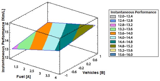
Figure 9.
Surface Response instantaneous performance analysis.
The axes represent different variables with the Fuel [A] axis ranging from 1 to 4 as we described in Table 2, and the Vehicles [B] axis ranging from −1 to 1, correlating with vehicle models such as the Hyundai Accent and Chevrolet Sail. The vertical axis quantifies the performance of these combinations in km/L, showcasing how fuel efficiency varies with changes in fuel type and vehicle model.
The analysis of instantaneous fuel performance for both the HA 1.6 L and CS 1.5 L vehicles reveals small differences between the OBD II and external tank measurement methods. For the HA 1.6 L vehicle using extra fuel, the OBD II method shows a performance of 13.242 km/L, while the external tank method records 13.077 km/L, resulting in a slight difference of 1.24%. Similarly, the CS 1.5 L vehicle shows a performance of 13.915 km/L with the OBD II method and 14.023 km/L with the external tank method, indicating a 0.77% difference. When using Ecopaís fuel, the HA 1.6 L vehicle achieves 14.376 km/L with the OBD II method and 14.491 km/L with the external tank method, demonstrating a minor difference of 0.79%. In contrast, the CS 1.5 L vehicle with the OBD II method records 15.195 km/L and with the external tank method, 15.077 km/L, showing a negligible difference of 0.78%. These results suggest that both measurement methods provide consistent instantaneous fuel performance readings with minimal variation.
The surface plot suggests that the optimal performance, indicated by the yellow color, is achieved with specific combinations of fuel and vehicle types. The CS 1.5 L vehicle generally exhibits better fuel efficiency than the HA 1.6 L vehicle with both types of fuel and measurement methods.
This helps to visualize how different combinations of vehicles and fuel types can impact fuel efficiency, with clear indications that certain conditions maximize performance. This is aligned with the document’s explanation that the Chevrolet Sail with Ecopaís fuel measured by an external tank shows the best performance in terms of fuel economy (lower fuel consumption per kilometer).
3.1.2. Long-Term Fuel Efficiency
Long-term fuel efficiency represents the average fuel consumption of a vehicle over an extended period or distance, typically measured in liters per 100 km (L/100 km). This metric provides a comprehensive view of a vehicle’s fuel efficiency. It reflects the total fuel consumed over a long journey or multiple trips, divided by the total distance traveled. Table 5 shows the results of the long-term fuel performance of the vehicles analyzed by using the Ecopaís and Extra fuels and with the way to measure them.
Table 5.
Long-term fuel performance.
In the assessment of long-term fuel performance, more pronounced differences are observed between the OBD II and external tank measurement methods. For the HA 1.6 L vehicle using extra fuel, the OBD II method shows a consumption of 7.5 L/100 km, whereas the external tank method indicates 7.7 L/100 km, resulting in a 2.59% difference. The CS 1.5 L vehicle exhibits a greater disparity, with the OBD II method recording 6.5 L/100 km and the external tank method showing 7.1 L/100 km, reflecting an 8.45% difference. When using Ecopaís fuel, the HA 1.6 L vehicle consumes 7 L/100 km with the OBD II method and 6.9 L/100 km with the external tank method, indicating a 1.43% difference. Similarly, the CS 1.5 L vehicle shows a consumption of 6.3 L/100 km with the OBD II method and 6.5 L/100 km with the external tank method, resulting in a 3.17% difference. These findings suggest that the long-term fuel performance measurements can be more sensitive to the chosen method, especially for certain vehicle and fuel combinations.
Figure 10 demonstrates that the best long-term fuel efficiency (lowest L/100 km) is achieved with specific combinations of vehicle and fuel types, shown in dark blue. This optimal combination likely involves the Chevrolet Sail using a higher quality or specific type of fuel, consistent with the findings from the instantaneous performance graph. Both vehicles show better long-term fuel efficiency with Ecopaís compared to Extra. There are slight differences between the OBD II and tank measurements, with the tank method generally showing marginally higher consumption. The CS 1.5 L vehicle shows significantly better long-term fuel efficiency, ranging from approximately 4.74% to 14%, depending on the fuel type and measurement method used.
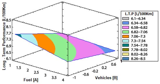
Figure 10.
Surface response long-term fuel performance analysis.
3.1.3. Conversion of Fuel Consumption to Energy Consumption
To convert the fuel consumption of a vehicle (in liters per 100 km) to energy consumption (in kWh per 100 km), we use the energy value per liter of gasoline. The process and the equations involved are described in the next steps:
- Calorific Value of the Fuel: The lower calorific value (LCV) of gasoline is the amount of energy released when one liter of gasoline is burned. This value ranges from 31.5 to 33.7 MJ/L [26,27].For our calculations, we use the average value:
- Conversion from [MJ] to [kWh]: To convert megajoules [MJ] to kilowatt-hours [kWh], the following relationship is used:
- Conversion of Fuel Consumption to Energy Consumption: To convert fuel consumption in liters per 100 km to energy consumption in kWh per 100 km, we use the following equation:
3.2. Energy Consumption of Nissan Leaf
The simulation of energy consumption for a Nissan Leaf, performed using MATLAB Simulink, appears to be a detailed analysis designed to understand how different driving conditions, specifically variations in terrain slopes, affect the vehicle’s battery life and overall performance.
Driving on these varied slopes has a profound impact on vehicle dynamics, primarily affecting energy consumption and regenerative braking. Uphill drives significantly increase power demand, thereby accelerating the depletion of the battery’s state of charge [28]. Conversely, downhill sections offer opportunities for regenerative braking, which can help recuperate some energy back to the battery, although its effectiveness diminishes on steeper slopes. These dynamics are critical for understanding how electric vehicles perform under different road conditions and are essential for optimizing energy management and vehicle stability in response to terrain changes.
The SOC for the Nissan Leaf electric vehicle simulation showed on Figure 11, reveals the battery’s charge depletion over time under two distinct conditions: driving with and without slope variations. In both scenarios, the SOC declines steadily from a full charge, but the decline is notably quicker when encountering slope variations, as evidenced by the steeper slope of the blue line in the graph. This quicker depletion is attributed to increased energy demands, especially when navigating uphill gradients that require more power to overcome gravitational forces.
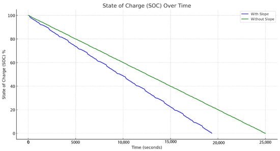
Figure 11.
State of charge battery Nissan Leaf 40 kW.
In the analyzed scenarios, both with and without slope variations, the energy consumption was remarkably similar—approximately 41 kWh—despite notable differences in the conditions. In the scenario with slope, the vehicle or system used slightly less energy (40.957 kWh) and covered a shorter distance of 207.77 km in about 5 h and 24 min, indicating higher energy demand due to the additional resistance from slopes. Conversely, the scenario without slope saw a slightly higher energy consumption (41.186 kWh) but achieved greater distance efficiency, covering 268.80 km in roughly 6 h and 56 min, demonstrating that flatter terrain allows for more efficient travel over longer distances due to reduced energy expenditure on overcoming gravitational forces (Table 6).
Table 6.
Nissan Leaf simulation results.
3.3. Comparative Analysis
The comparative analysis between combustion vehicles and electric vehicles like the Nissan Leaf is conducted by examining their energy consumption in terms of kWh per 100 km. This metric effectively measures the amount of energy each vehicle type uses to travel a specific distance, highlighting the efficiency of energy conversion from fuel or electricity to mechanical motion.
3.3.1. Combustion Vehicles Analyzed
The research provides long-term energy efficiency in liters per 100 km for the HA 1.6 L and CS 1.5 L vehicles using different types of fuel. However, to provide specific values in kWh per 100 km, it is necessary to convert the L/100 km values to kWh/100 km using an appropriate conversion factor.
Below in Table 7, the energy efficiency is expressed in L/100 km. To convert from L/100 km to kWh/100 km, a common conversion factor for gasoline (Equation (14)) will be used, and the resultant energy efficiency per vehicle and fuel consumed is shown in the column energy efficiency. These values indicate how much energy in kilowatt-hours the vehicles would consume per 100 km traveled, depending on the type of fuel used.
Table 7.
Energy efficiency of combustion vehicles.
3.3.2. Nissan Leaf Simulation
The energy efficiency in kWh per 100 km can be calculated using the total energy consumed and the final distance traveled. The formula we will use is
From the provided data:
- Energy consumed = 40.95 kWh;
- Distance traveled = 207,773.74 m.
First, the distance will be converted from meters to kilometers. Then, the formula will be applied to calculate the energy efficiency in kWh per 100 km. These calculations will now be performed, resulting in an energy efficiency of approximately 19.71 kWh per 100 km.
3.4. Performance
The comparative analysis highlights that combustion vehicles like the HA 1.6 L (Hyundai Accent) and CS 1.5 L (Chevrolet Sail) are less efficient in energy consumption, displaying higher kWh usage per 100 km. This inefficiency is primarily due to the nature of combustion engines, which have significant energy losses in the process of converting fuel energy into mechanical energy. These vehicles embody the traditional challenges associated with internal combustion engines, including lower conversion efficiency and higher operational costs due to fuel consumption.
On the other hand, the Nissan Leaf, an electric vehicle, demonstrates significantly better energy efficiency, consuming approximately 15 to 20 kWh per 100 km. This stark contrast in energy consumption underscores the advantages of electric vehicles, which are able to convert electrical energy directly into mechanical energy with much higher efficiency. Electric vehicles like the Nissan Leaf avoid the thermal losses common in combustion processes, showcasing why EVs are increasingly seen as more sustainable and cost-effective alternatives to traditional fuel-based vehicles.
4. Discussion
4.1. Energy Efficiency
The discussion on energy efficiency between the analyzed combustion vehicles (Hyundai Accent 1.6 L and Chevrolet Sail 1.5 L) and a simulated Nissan Leaf centers on their respective abilities to convert their energy sources into vehicle motion efficiently. This comparison is pivotal in illustrating the intrinsic advantages of electric vehicles (EVs) over traditional combustion engine vehicles.
Combustion vehicles such as the Hyundai Accent and Chevrolet Sail typically exhibit energy consumption rates around 56.96 to 61.86 kWh per 100 km when converted from their fuel consumption in liters. These values are considerably higher compared to electric vehicles. This disparity stems from the fundamental inefficiencies inherent in combustion engines where a significant portion of the energy from fuel is lost as heat instead of being converted into mechanical energy. Additionally, the mechanical complexities of transmissions and drivetrains in combustion vehicles further reduce their energy efficiency.
In stark contrast, the Nissan Leaf, representative of modern electric vehicles, generally consumes between 15 and 20 kWh per 100 km, showcasing a much more efficient use of energy. The efficiency of electric vehicles comes from their direct conversion of electricity into motion with minimal energy loss, bypassing the inefficiencies of combustion processes and complex drivetrains. EVs benefit from simpler mechanisms that allow for a more straightforward energy path from the battery to the wheels.
4.2. Environmental Impact
Electric vehicles (EVs), like the Nissan Leaf, provide substantial environmental benefits compared to traditional internal combustion engine (ICE) vehicles. This is primarily due to their higher energy efficiency and zero tailpipe emissions. EVs are able to convert over 60% of the electrical energy from the grid into power at the wheels, significantly reducing waste and increasing the overall efficiency of energy usage [29]. When powered by renewable energy sources, EVs can achieve near-zero lifecycle emissions, sharply decreasing their environmental impact. The production of EV batteries does introduce environmental challenges, including the extraction of raw materials like lithium and cobalt. However, ongoing advancements in battery technology and recycling processes are continually reducing these impacts.
In contrast, combustion engine vehicles are less efficient, converting only about 20–30% of the energy stored in gasoline into power at the wheels, with the rest being lost as heat [30]. This inefficiency necessitates higher fuel consumption and leads to greater emissions of CO2, NOx, and other pollutants, contributing to climate change and air quality issues. Additionally, the entire lifecycle of ICE vehicles, from oil extraction to fuel consumption, imposes significant environmental burdens, including oil spills, land degradation, and water contamination. Although ICE vehicles can be recycled, their operational emissions and the continual need for fossil fuels weigh heavily on their environmental footprint, making EVs like the Nissan Leaf a more sustainable choice in the drive toward reducing automotive emissions and advancing global sustainability goals.
For internal combustion engine (ICE) vehicles, the total greenhouse gas (GHG) emissions over a typical gasoline-powered car’s lifetime, including manufacturing, fuel production, and operation, can amount to approximately 24 tons of CO2 equivalent (CO2e). These emissions arise from the various stages of the vehicle’s lifecycle, with a significant portion attributed to fuel combustion during operation, which consistently generates CO2 and other pollutants. Manufacturing and fuel production also contribute notably to the overall emissions, highlighting the comprehensive environmental impact of traditional gasoline vehicles [31].
In contrast, electric vehicles (EVs) present a different emissions profile. On average, a mid-sized EV like the Nissan Leaf results in around 12 tons of CO2e over its lifetime when considering a typical electricity mix. This reduction is primarily due to the higher efficiency of electric motors and the potential for lower emissions during electricity production compared to gasoline combustion. If the electricity used for charging is sourced entirely from renewable energy, the total lifetime emissions for the same EV can be reduced further to approximately 6 tons of CO2e. This significant decrease emphasizes the environmental benefits of using renewable energy sources for EV charging and showcases the potential for substantial reductions in GHG emissions through the adoption of electric vehicles and clean energy [32,33,34].
4.3. Operational Cost
To analyze and compare the cost of fueling the analyzed combustion vehicles (Hyundai Accent 1.6 L and Chevrolet Sail 1.5 L) with Extra and Ecopaís gasoline and charging a simulated Nissan Leaf electric vehicle under the new pricing regime, let us calculate the cost of filling their tanks and battery.
Combustion Vehicles: The Hyundai Accent 1.6 L has a fuel tank capacity of approximately 45 L (11.9 gallons) [35], making it well suited for both city and highway driving. On the other hand, the Chevrolet Sail 1.5 L features a slightly smaller fuel tank with a capacity of around 43 L [36]. These capacities are standard for these models and provide a good balance between driving range and vehicle size, ensuring efficient fuel use for both daily commutes and longer journeys. The price for Extra and Ecopaís gasoline has increased to USD 2.722 per gallon [37]; with these data, the operating cost to travel 100 km is shown in Table 8, where the vehicle with the highest cost to fill the fuel tank is the Hyundai Accent, regardless of whether it uses Extra or Ecopaís fuel, with a total cost of USD 32.36 for a full tank.
Table 8.
Cost to fill the fuel tank of combustion vehicles.
Electric Vehicle (Nissan Leaf): Assume the Nissan Leaf has a battery capacity of 40 kWh, typical for recent models. The price for electricity is stated as 28 cents per kWh [38,39]. The cost to fully charge the battery of a Nissan Leaf, which has a capacity of 40 kWh, is USD 11.20 (Table 9).
Table 9.
Cost to charge the battery of the Nissan Leaf.
Charging the Nissan Leaf is significantly more cost-effective compared to filling the fuel tank of combustion vehicles. This lower cost of electricity for EVs highlights one of the primary economic advantages of electric vehicles over traditional combustion engine vehicles, making them a more attractive option for cost-conscious consumers.
4.3.1. Fuel Cost Calculations
The vehicle with the highest operating cost per 100 km is the Hyundai Accent using Extra fuel, with a cost of USD 5.47 per 100 km. This cost is slightly higher than that of the Nissan Leaf when considering the upper end of its electricity consumption range (USD 5.60 per 100 km), as is shown in Table 10.
Table 10.
Comparison of operating costs to travel 100 km.
4.3.2. Maintenance Cost Calculations
For the electric vehicle, maintenance costs include replacing shock absorbers at USD 200 every 60,000 km, replacing tires at USD 280 every 50,000 km, and replacing brake pads at USD 200 every 50,000 km. These components are necessary due to natural wear and tear during driving. An additional significant cost is the battery replacement at 300,000 km, which amounts to USD 12,000 [40,41]. In total, the maintenance costs for the electric vehicle amount to USD 15,880 at 300,000 km. For the internal combustion engine vehicle, maintenance costs include oil changes that occur every 5000 km at a cost of USD 40 each, replacing shock absorbers at USD 200 every 60,000 km, replacing tires at USD 280 every 50,000 km, and replacing brake pads at USD 200 every 50,000 km. Additionally, this vehicle requires an engine repair at 300,000 km, costing USD 2000. In total, the maintenance costs for the internal combustion engine vehicle amount to USD 8280 at 300,000 km, as is shown in Figure 12.
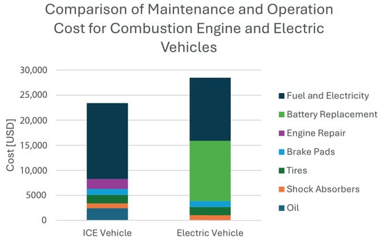
Figure 12.
Comparison of maintenance and operation cost for an ICE vehicle and electric vehicle up to a lifetime of 300,000 km estimation in Ecuador.
When analyzing the fuel and energy costs for covering 300,000 km, it is observed that the Nissan Leaf, an electric vehicle, has the lowest cost at USD 12,600. In comparison, internal combustion vehicles have significantly higher costs: the HA 1.6 L with Extra fuel reaches USD 16,555, while with Ecopaís fuel, it is USD 14,775; the CS 1.5 L with Extra fuel costs USD 15,261 and with Ecopaís fuel, it is USD 14,074. The average fuel cost for internal combustion vehicles is USD 15,166.25, highlighting the economic advantage of electric vehicles in terms of long-term operating costs.
The cost estimates used in this analysis are based on the current prices for tires, oil, and brake pads in Ecuador, and do not include labor costs. These costs can vary from country to country and depending on the brand. Therefore, the actual maintenance costs may differ based on geographical location and the specific brands of components used.
4.4. Limitations
The adoption and efficient use of electric vehicles (EVs) in Ecuador face several challenges, primarily due to the country’s geographical and infrastructural factors. This analysis considers the difficulties posed by the country’s rugged terrain, the existing state of charging infrastructure, and the capability of hydroelectric power to support EVs.
Geographical Challenges: Ecuador’s diverse terrain, characterized by the Andes mountains and significant variations in elevation, presents unique challenges for electric vehicles.
Slope Variation: EVs typically consume more energy on steep slopes, which are common in mountainous regions like the Andes. This can significantly reduce the range of EVs, necessitating more frequent charges and potentially affecting the overall efficiency and practicality of EVs in such regions.
Impact on Battery Life: Frequent climbing and descending in mountainous areas can lead to more rapid battery degradation due to the increased load and discharge cycles.
Charging Infrastructure: The availability and distribution of EV charging stations are essential for the adoption of electric vehicles.
Number of Chargers: Ecuador has a limited number of EV charging stations, concentrated mainly in urban areas like Quito and Guayaquil. The limited availability can be a significant barrier, especially for long-distance travel across less-urbanized areas.
Distribution of Chargers: The uneven distribution of charging stations means that there are significant gaps in the EV charging network, particularly in rural or less developed areas. This lack of infrastructure can deter the use of EVs, especially for those living outside major cities or those who frequently travel long distances.
Hydroelectric Power and Energy Supply: Ecuador relies heavily on hydroelectric power, which accounts for a significant portion of its energy production.
Energy Production Capacity: Ecuador’s hydroelectric plants have been a major power source, supporting the nation’s push towards renewable energy. However, the capacity to expand and the reliability of these sources can be impacted by seasonal variations and climate change.
Sufficiency for EVs: While hydroelectric power is a clean energy source ideal for supporting an electric vehicle network, the overall energy demands must be assessed to ensure there is enough capacity to handle the increased load from widespread EV adoption. If every vehicle owner switched to electric, the existing infrastructure and energy supply might struggle to meet the heightened demand without significant upgrades.
5. Conclusions
The energy efficiency comparison between combustion vehicles (Hyundai Accent 1.6 L and Chevrolet Sail 1.5 L) and the Nissan Leaf underscores significant differences in how each vehicle type utilizes energy. The combustion vehicles, with energy consumption rates of 56.96 to 61.86 kWh per 100 km when converted from their fuel use, exhibit inherent inefficiencies typical of internal combustion engines. These inefficiencies arise from the loss of a substantial portion of energy as heat and through the mechanical complexities involved in converting fuel energy to motion. Consequently, these vehicles are not only less energy efficient but also more expensive to operate due to higher fuel costs, which are exacerbated by rising gasoline prices as seen with the recent price increase to USD 2.722 per gallon in Ecuador.
In contrast, the Nissan Leaf, an electric vehicle, consumes between 15 and 20 kWh per 100 km, reflecting its superior energy efficiency. This efficiency translates directly into cost savings, with the Leaf costing significantly less to “fuel” per 100 km—as demonstrated by the comparison of filling a 40 L tank for combustion vehicles versus fully charging a 40 kWh Nissan Leaf battery. With the Leaf’s electricity cost being only USD 11.20 to reach full charge, it presents a more economical option over the long term, especially considering the rising costs of gasoline. Despite these advantages, the adoption and practicality of electric vehicles like the Nissan Leaf in Ecuador face several challenges. The geographical diversity, particularly the mountainous terrain, affects the practical range of EVs and can accelerate battery degradation due to constant high-load conditions. Moreover, the current EV charging infrastructure in Ecuador is insufficient and unevenly distributed, primarily concentrated in major urban centers such as Quito and Guayaquil. This limitation is critical for potential EV users in rural or less developed areas and for inter-city connectivity where charging options are sparse.
Looking forward, for Ecuador to fully leverage the benefits of electric vehicles, there needs to be a concerted effort to expand and evenly distribute the charging infrastructure. This expansion should particularly focus on areas that currently lack sufficient access to ensure that EVs are a viable option across the entire country. Additionally, as the reliance on electric vehicles grows, it will be crucial to assess and possibly expand the hydroelectric and other renewable energy capacities to meet the increased electricity demand. This expansion is essential not only to maintain the environmental benefits of electric vehicles but also to ensure the stability and sustainability of the national energy grid.
While the Nissan Leaf and potentially other electric vehicles offer a more energy-efficient and cost-effective solution compared to traditional combustion vehicles, their widespread adoption in Ecuador will require strategic planning, significant investment in infrastructure, and an ongoing evaluation of the energy supply chain. Addressing these issues will help overcome current limitations and pave the way for a more sustainable and economically beneficial implementation of electric vehicles in Ecuador’s diverse geographical and economic landscape.
Future work will involve conducting the study at sea level to enable a more accurate comparison and to better understand the effects of altitude on energy efficiency for both combustion and electric vehicles. This comprehensive analysis will provide deeper insights into optimizing vehicle performance across different terrains and altitudes.
Author Contributions
Conceptualization, D.S.P.-B., M.I.Q.-M. and A.S.C.-C.; writing—original draft preparation, A.G.M.-Y.; writing—review and editing, R.R.M.-P., F.A.M. and H.G.U.-G.; visualization, F.A.M.; supervision, D.S.P.-B. and M.I.Q.-M. All authors have read and agreed to the published version of the manuscript.
Funding
This research received no external funding.
Data Availability Statement
The original contributions presented in the study are included in the article; further inquiries can be directed to the corresponding author.
Acknowledgments
We thank the Escuela Superior Politécnica de Chimborazo ESPOCH, Instituto Superior Tecnológico Tungurahua and Universidad de las Fuerzas Armadas ESPE.
Conflicts of Interest
Fernando Alejandro Murillo is an employee of Safe Risk Insurance Brokers Pvt. Ltd. The paper reflects the views of the scientists, and not the company.
Abbreviations
The following abbreviations are used in this manuscript:
| ICE | Internal combustion engine |
| EV | Electric vehicle |
| ELM327 | Electronic device for OBD II data acquisition |
| ECU | Engine control unit |
| OBD II | On-board diagnostic system |
| PSI | Pounds per square inch |
References
- IPCC. Section 4: Near-Term Responses in a Changing Climate; Climate Change 2023: Synthesis Report; IPCC: Geneva, Switzerland, 2023; pp. 42–66. [Google Scholar] [CrossRef]
- IEA. Electricity 2024 Analysis and Forecast to 2026; International Energy Agency: Paris, France, 2023; pp. 1–170. [Google Scholar]
- Ashnani, M.H.M.; Miremadi, T.; Johari, A.; Danekar, A. Environmental Impact of Alternative Fuels and Vehicle Technologies: A Life Cycle Assessment Perspective. Procedia Environ. Sci. 2015, 30, 205–210. [Google Scholar] [CrossRef]
- Department of Energy. Electric Vehicles; Department of Energy: Washington, DC, USA, 2022. [Google Scholar]
- Liang, F.; Zhang, L. Effects of Altitude on Power Performance of Commercial Vehicles. OALib 2018, 5, 1–8. [Google Scholar] [CrossRef]
- Liu, Z.; Liu, J. Effect of altitude conditions on combustion and performance of a turbocharged direct-injection diesel engine. Proc. Inst. Mech. Eng. Part D J. Automob. Eng. 2022, 236, 582–593. [Google Scholar] [CrossRef]
- Jiang, Z.; Wu, L.; Niu, H.; Jia, Z.; Qi, Z.; Liu, Y.; Zhang, Q.; Wang, T.; Peng, J.; Mao, H. Investigating the impact of high-altitude on vehicle carbon emissions: A comprehensive on-road driving study. Sci. Total Environ. 2024, 918, 170671. [Google Scholar] [CrossRef] [PubMed]
- Deng, Y. Future Vehicle Trend: A Comparative Study of the Fuel Vehicle, Electrical Vehicle, and Hybrid Vehicles. Highlights Sci. Eng. Technol. 2023, 29, 143–148. [Google Scholar] [CrossRef]
- Ministerio de Energia y Minas. Ecuador Consolida la Producción Eléctrica a Partir de Fuentes Renovables; Ministerio de Energia y Minas: Santo Domingo, Dominican Republic, 2019. [Google Scholar]
- International Trade Administration—Electric Power and Renewable Energy. Available online: https://www.trade.gov/country-commercial-guides/ecuador-electric-power-and-renewable-energy (accessed on 7 July 2024).
- Comité de Comercio Exterior (COMEX). Resolución COMEX 016-2019. 2019. Available online: https://www.produccion.gob.ec/wp-content/uploads/2019/06/RESOLUCIO%CC%81N-COMEX-016-2019.pdf (accessed on 4 July 2024).
- Qi, Z.; Gu, M.; Cao, J.; Zhang, Z.; You, C.; Zhan, Y.; Ma, Z.; Huang, W. The Effects of Varying Altitudes on the Rates of Emissions from Diesel and Gasoline Vehicles Using a Portable Emission Measurement System. Atmosphere 2023, 14, 1739. [Google Scholar] [CrossRef]
- Ceballos, J.J.; Melgar, A.; Tinaut, F.V. Influence of environmental changes due to altitude on performance, fuel consumption and emissions of a naturally aspirated diesel engine. Energies 2021, 14, 5346. [Google Scholar] [CrossRef]
- Mamarikas, S.; Doulgeris, S.; Samaras, Z.; Ntziachristos, L. Traffic impacts on energy consumption of electric and conventional vehicles. Transp. Res. Part D Transp. Environ. 2022, 105, 103231. [Google Scholar] [CrossRef]
- Boggio-Marzet, A.; Monzon, A.; Rodriguez-Alloza, A.M.; Wang, Y. Combined influence of traffic conditions, driving behavior, and type of road on fuel consumption. Real driving data from Madrid Area. Int. J. Sustain. Transp. 2022, 16, 301–313. [Google Scholar] [CrossRef]
- Rocha-Hoyos, J.C.; Tipanluisa, L.E.; Zambrano, V.D.; Portilla, Á.A. Study of a gasoline engine in altitude conditions with mixtures containing organic additive in the fuel. Inf. Tecnol. 2018, 29, 325–334. [Google Scholar] [CrossRef]
- Pereira, A.; Alves, M.; Macedo, H. Vehicle driving analysis in regards to fuel consumption using Fuzzy Logic and OBD-II devices. In Proceedings of the 2016 8th Euro American Conference on Telematics and Information Systems, EATIS 2016, Cartagena, Colombia, 28–29 April 2016. [Google Scholar] [CrossRef]
- Abukhalil, T.; Almahafzah, H.; Alksasbeh, M.; Alqaralleh, B.A. Fuel Consumption Using OBD-II and Support Vector Machine Model. J. Robot. 2020, 2020, 9450178. [Google Scholar] [CrossRef]
- EluniversoGasolina. Estas son las Ventajas y Desventajas de Usar las Gasolinas Ecopaís y Extra en Ecuador | Economía | Noticias | El Universo. Available online: https://www.eluniverso.com/noticias/economia/estas-son-las-ventajas-y-desventajas-de-usar-las-gasolinas-ecopais-y-extra-en-ecuador-nota/ (accessed on 8 July 2024).
- EP PETROECUADOR. Loja Cuenta con Ecopaís, una Gasolina Amigable Con el Medio Ambiente—EP PETROECUADOR. Available online: https://www.eppetroecuador.ec/?p=5254 (accessed on 8 July 2024).
- Puma-Benavides, D.S.; Izquierdo-Reyes, J.; Galluzzi, R.; Calderon-Najera, J.d.D. Influence of the final ratio on the consumption of an electric vehicle under conditions of standardized driving cycles. Appl. Sci. 2021, 11, 11474. [Google Scholar] [CrossRef]
- Wong, J.Y. Theory of Ground Vehicles; Wiley-Interscience: Hoboken, NJ, USA, 2001; p. 528. [Google Scholar]
- Mohan, G.; Assadian, F.; Longo, S. Comparative analysis of forward-facing models vs backwardfacing models in powertrain component sizing. In Proceedings of the IET Hybrid and Electric Vehicles Conference 2013 (HEVC 2013), London, UK, 6–7 November 2013; pp. 1–6. [Google Scholar]
- Bamdezh, M.A.; Molaeimanesh, G.R. Aging behavior of an electric vehicle battery system considering real drive conditions. Energy Convers. Manag. 2024, 304, 118213. [Google Scholar] [CrossRef]
- Zhang, R.; Yao, E. Electric vehicles’ energy consumption estimation with real driving condition data. Transp. Res. Part D Transp. Environ. 2015, 41, 177–187. [Google Scholar] [CrossRef]
- Iliev, S. A Comparison of Ethanol, Methanol, and Butanol Blending with Gasoline and Its Effect on Engine Performance and Emissions Using Engine Simulation. Processes 2021, 9, 1322. [Google Scholar] [CrossRef]
- Zhang, Z.; Wu, F. Adaptive Equivalent Fuel Consumption Minimization Based Energy Management Strategy for Extended-Range Electric Vehicle. Sustainability 2023, 15, 4607. [Google Scholar] [CrossRef]
- Li, W.; Stanula, P.; Egede, P.; Kara, S.; Herrmann, C. Determining the Main Factors Influencing the Energy Consumption of Electric Vehicles in the Usage Phase. Procedia CIRP 2016, 48, 352–357. [Google Scholar] [CrossRef]
- Carbonbrief Org. Factcheck: How Electric Vehicles Help to Tackle Climate Change. Available online: https://www.carbonbrief.org/factcheck-how-electric-vehicles-help-to-tackle-climate-change/ (accessed on 8 July 2024).
- Pike, B.Y.E. Calculating Electric Drive Vehicle Greenhouse Gas Emissions; International Council on Clean Transportation: Washington, DC, USA, 2012. [Google Scholar]
- US EPA. Greenhouse Gas Emissions from a Typical Passenger Vehicle; US EPA: Washington, DC, USA, 2023. [Google Scholar]
- US EPA. Comparison: Your Car vs. an Electric Vehicle; US EPA: Washington, DC, USA, 2024. [Google Scholar]
- Ellingsen, L.A.W.; Singh, B.; Strømman, A.H. The size and range effect: Lifecycle greenhouse gas emissions of electric vehicles. Environ. Res. Lett. 2016, 11, 054010. [Google Scholar] [CrossRef]
- Hao, H.; Mu, Z.; Jiang, S.; Liu, Z.; Zhao, F. GHG Emissions from the production of lithium-ion batteries for electric vehicles in China. Sustainability 2017, 9, 504. [Google Scholar] [CrossRef]
- Carspecs. Hyundai Accent Gas Tank Size; Carspecs: Downey, CA, USA, 2022. [Google Scholar]
- Autopadre. Hyundai Accent Gas Tank Size (2002–2022): Fuel Tank Capacity Data; Autopadre: Botosani, Romania, 2022. [Google Scholar]
- GlobalPetrolPrices. Ecuador Precios de la Gasolina. Available online: https://es.globalpetrolprices.com/Ecuador/gasoline_prices/ (accessed on 22 July 2024).
- Recursos y Energia Costo 2023. Costo de la Tarifa eléCtrica se Mantiene para Sectores Residencial y Comercial; Industriales Recibirán Incentivos por Autogeneración de Energía; Ministerio de Energia y Minas: Quito, Ecuador, 2024. [Google Scholar]
- EEQ. El Precio del Kilovatio Hora es Único en Todos los Sectores: La Empresa elÉctrica Quito te lo Explica; Empresa Eléctrica Quito-Empresa Electrica Quito: Quito, Ecuador, 2023. [Google Scholar]
- Aliexpress. Batería Original de 40kwh Para Nissan Leaf, Milage120km–130km para Correr; AliExpress: Hangzhou, China, 2023. [Google Scholar]
- NissanLeafevaluation. AnÁlisis de las BaterÍas del Nissan Leaf 40 kWh tras 5 AÑOS|by Iván Ballestín Nuez|Medium; Nissan: Yokohama, Japan, 2022. [Google Scholar]


Disclaimer/Publisher’s Note: The statements, opinions and data contained in all publications are solely those of the individual author(s) and contributor(s) and not of MDPI and/or the editor(s). MDPI and/or the editor(s) disclaim responsibility for any injury to people or property resulting from any ideas, methods, instructions or products referred to in the content. |
© 2024 by the authors. Licensee MDPI, Basel, Switzerland. This article is an open access article distributed under the terms and conditions of the Creative Commons Attribution (CC BY) license (https://creativecommons.org/licenses/by/4.0/).