Abstract
Plug-in hybrid electric vehicles (PHEVs) are designed to enable the electrification of a large portion of the distance vehicles travel while utilizing relatively small batteries via taking advantage of the fact that long-distance travel days tend to be infrequent for many vehicle owners. PHEVs also relieve range anxiety through seamless switching to hybrid driving—an efficient mode of fuel-powered operation—whenever the battery reaches a low state of charge. Stemming from the perception that PHEVs are a well-rounded solution to reducing greenhouse gas (GHG) emissions, various metrics exist to infer the effectiveness of GHG reduction, with utility factor (UF) being prominent among such metrics. Recently, articles in the literature have called into question whether the theoretical values of UF agree with the real-world performance of PHEVs, while also suggesting that infrequent charging was the likely cause for observed deviations. However, it is understood that other reasons could also be responsible for UF mismatch. This work proposes an approach that combines theoretical modeling of UF under progressively relaxed assumptions (including the statistical distribution of daily traveled distance, charging behavior, and attainable electric range), along with vehicle data logs, to quantitatively infer the contributions of various real-world factors towards the observed mismatch between theoretical and real-world UF. A demonstration of the proposed approach using data from three real-world vehicles shows that all contributing factors could be significant. Although the presented results (via the small sample of vehicles) are not representative of the population, the proposed approach can be scaled to larger datasets.
1. Introduction
Electric drive vehicles [1], also known as electrified vehicles [2], are a broad category of powertrains that were introduced into modern-day personal transportation systems more than two decades ago to reduce greenhouse gas (GHG) emissions as well as the reliance on petroleum-derived fuels. Loosely understood as vehicles whose traction power can be completely or partially provided via one or more electric motors. Earlier sub-categories of those powertrains included (non-plug-in) hybrid electric vehicles (HEVs), plug-in hybrid electric vehicles (PHEVs), and battery-only electric vehicles (BEVs). Later arrivals to the market included hydrogen-powered [3] fuel cell electric vehicles (FCEVs), which could be thought of as HEVs but with a fuel cell (FC) instead of an internal combustion engine (ICE), as well as plug-in fuel cell electric vehicles (PFCEVs), which could be thought of as PHEVs but with an FC instead of an ICE. One common trait among all such powertrains is the ability to provide acceleration power to the vehicle via electric motors powered by energy buffered or stored in a traction battery and, thus, gain efficiency advantages from the electric motor’s ability to operate at high efficiency across a broad range of torque and speed requirements, as opposed to an internal combustion engine, whose efficient operation tends to be limited to a rather narrow range of torque and speed. Another common feature of electrified powertrains is regenerative braking, which is the ability to recapture energy and store it back into the battery during vehicle braking events via operating the motor(s) as electric generators, using their negative torque to assist in the deceleration of the vehicle. With those two traits alone, HEVs can achieve appreciable reductions in fuel consumption (and corresponding reductions in GHG emissions) compared to conventional internal combustion engine (CICE) vehicles.
Other types of electrified powertrains aim to reduce GHG emissions further beyond the capability of HEVs in different ways. BEVs, which have no ICE, rely on a much larger battery designed to provide all the required energy for vehicle trips without relying on any other energy source, and only charging the battery from the electric grid in-between trips (while the vehicle is parked). As such, BEVs have no tailpipe emissions while driving, but their use phase emissions associated with electricity consumption from the grid may not be trivial, depending on location [4,5,6]. BEVs have excellent GHG reduction potential as power grids shift to a lower carbon electricity generation mix. However, perceptions about vehicle range, charging infrastructure availability, and charging time [7,8,9], as well as cost and resource material requirements due to larger-sized batteries [10,11,12,13], pose challenges to widespread adoption of BEVs in the short term. Hydrogen-powered vehicles share similar traits to BEVs in that they have no tailpipe emissions and future potential for excellent GHG reduction despite most of the present-day commercially available hydrogen coming from GHG-emitting sources, such as natural gas reforming [14]. While FCEVs have an advantage over BEVs in terms of refueling time, much like BEVs, infrastructure availability and cost issues [14,15] hinder the widespread adoption of FCEVs in the short term.
Aiming to reduce GHG emissions beyond HEVs, PHEVs are conceptually designed as a compromise between BEVs and HEVs in a manner that attains some of the attractive qualities of both. Equipped with the capability to charge from the electric grid (like BEVs, unlike HEVs) and appropriately sized batteries, PHEVs aim to electrify a large portion of vehicle travel distance on most days, while seamlessly transitioning to fuel power (operating as fuel-efficient HEVs) when the battery energy becomes low. In other words, PHEVs aim to relieve vehicle owners from relying on charging infrastructure and alleviate range anxiety issues when traveling long distances, while also electrifying an appreciable portion of the distance traveled and requiring less amounts of battery materials. In worst conditions, PHEVs operate nearly as efficiently as equivalent HEVs. In earlier studies in the literature involving theoretical and simulation-based work [16,17,18,19,20,21,22], PHEVs showed excellent potential for GHG emission reduction. However, more recent studies that focused on estimated real-world performance [23,24] questioned whether PHEVs are truly living up to their estimated GHG emission reduction benefits. Although further studies [25,26,27] suggested that the shortfall between modeled and real-world performances may not be as bad as initially estimated in [23,24], quantification of such a shortfall remains an open issue. Moreso, quantification of the contributions of various real-world factors toward differences between modeled and real-world performances has been seldom tackled in the literature and is the main focus of this paper.
When regulatory agencies around the world consider GHG certification of PHEVs, the certification process often relies on what is known as the utility factor (UF), which is defined in SAE J2841 standard [28] as the ratio of a PHEV distance traveled in charge depletion (CD) mode to its total traveled distance. CD mode refers to when the PHEV primarily relies on energy from the battery (hence, “depleting” the charge) for vehicle propulsion and operation. By making several idealization assumptions, UF curves (examples shown in Figure 1) provide a simplified means to estimating the expected UF of a PHEV solely as a function of its electric driving range (EDR), and the estimated UF can be further utilized toward estimates of the expected GHG emissions for the PHEV.
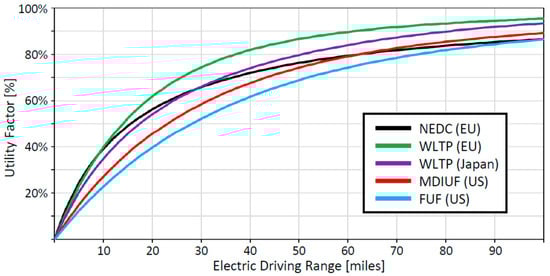
Figure 1.
Utility factor curves from select standards.
Needless to say, the assumptions enabling the derivation of a UF curve impact what the curve turns out to be, which is why different standard UF curves exist. For example, the older European Union (EU) standard, which relied on NEDC test procedures [29] (whose UF curve formula is outlined in [30]), assumes that a PHEV will deplete its battery and then drive an average distance of 25 km in charge-sustaining (CS) mode before being fully recharged. CS mode is the other main (but not the only other) mode of operation for a PHEV, during which, the ICE is the main source of power. In CS mode, the charge level in the battery is maintained between operating margins (hence, “sustaining” the charge). On the other hand, SAE J2841 standard [28] makes a different set of assumptions including that PHEVs are fully charged overnight before every driving day and do not charge during the day. UF estimates as function of EDR are conducted based on the population-wide statistical distribution of the distance traveled per day, with such statistical distribution coming from travel surveys of real vehicles [31]. The Worldwide Harmonized Light Vehicle Test Procedure (WLTP) [32], which became the EU standard succeeding NEDC, and also adopted in Japan and other places around the world, applied the same principal assumptions from SAE J2841 but used different travel survey data, resulting in different probabilities of days with travel distances exceeding the range of the PHEV, leading to different UF curves (as shown in Figure 1).
It is perhaps noteworthy that there were not many PHEVs driving on the road at the time of development of those standards (typically a few years prior to the publication date of the standards). As such, the daily travel distance data in the travel surveys mainly came from CICE vehicles, with the development of UF curves being primarily an answer to the question “what would be the CD mode fraction if a PHEV (with given EDR) had done the same trips while starting the day with a full battery?” It is also noteworthy that all the aforementioned standards implicitly assume that PHEVs attain their estimated EDR and no explicit treatment exists in those standards to account for variation in the actual/attained range that occurs due to variations in the driving conditions. Lastly, it is also noteworthy to mention that the SAE J2841 standard makes a distinction (hence, two different UF curves) between the multi-day individual utility factor (MDIUF) and fleet utility factor (FUF). MDIUF aims to estimate the UF of a randomly picked sample PHEV within a population, and it is calculated as a simple average of the UF estimated for vehicle samples in a travel survey dataset. FUF on the other hand, aims to estimate the overall fraction of distance traveled in CD mode from all vehicles combined, which amounts to a weighted average of the UF for each vehicle sample in the travel survey by its total traveled distance. FUF typically has a lesser value than MDIUF at any given value of EDR (as in Figure 1) because vehicle samples that travel longer distances tend to have lower UF.
Raghavan and Tal [33,34] presented some of the earlier literature work that attempted to determine the different reasons for mismatch between real-world UF and the standard curves. Theoretical modeling of alternative charging behaviors was also considered in [35]. As illustrated in Figure 2, the broad categories of reasons for UF mismatch include: (i) mismatch in the distribution of daily traveled distance, (ii) mismatch between the actual/achieved EDR and the rated one, (iii) mismatch between actual and assumed charging behaviors, and (iv) other reasons.
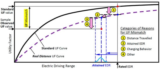
Figure 2.
Illustration of the main categories of reasons for utility factor mismatch.
For illustration simplicity, Figure 2 shows all categories of reasons for UF mismatch pointing in the same direction, where the real-world UF is less than the standard curves. However, it is noted that some of those real-world factors could work in the opposite direction. For example, if a PHEV is charged more than once per day, then one expects the arrow symbolizing the contribution of charging behavior in Figure 2 to be pointing upwards rather than downwards. Similarly, if the distribution of the daily travel distance had more short distance days than the standard, then the “real distance UF curve” would be above (i.e., larger UF values given EDR) the standard UF curve in Figure 2, much like how the standard UF curves in other parts of the world compare to the standard UF curves in the US.
One of the notable points emphasized in Figure 2 (compared to similar previous illustrations in the literature [25,35]) pertains to how the attained EDR is treated as a variable quantity that changes from trip to trip rather than one average value. This is because, on any given trip, the attainable electric driving distance is a combined function of: (i) total trip distance, (ii) battery state of charge (SOC) at the beginning of the trip, and (iii) attained EDR during the trip (not some long-term average). Another notable treatment in Figure 2 is the separation of “other reasons” from the three other categories of reasons instead of lumping with charging behavior or attained EDR. “Other reasons” is a catch-all category that encompasses anything that could not be attributed to the three other categories, such as errors/imperfections in real-world data measurements. Other reasons also include complexities introduced by “blended operation”, where some PHEVs (due to reasons such as cold weather or higher power demand) may turn on the engine while in CD mode. In the definition of UF in SAE J2841 standard [28], all distance traveled in CD mode (whether the engine is on or off) is counted toward the UF. However, since blended mode often involves vehicle power demand coming from both the engine and battery at the same time, neither “including all” nor “excluding all” of the distance traveled in CD mode with the engine on would be an exact estimate of the true fraction of the PHEV distance traveled that has been electrified via grid power.
This paper began with an overview and motivation for the research, as well as a brief review of relevant and related literature. Section 2 provides details of vehicle data logs and the proposed analysis approach. Section 3 presents a summary of results along with a discussion, which then leads to the conclusion of the paper. The perceived contributions include the following:
- (i)
- Developing a computationally scalable approach for utilizing real-world vehicle data logs toward estimating the share of contributions of the various categories of reasons for UF mismatch.
- (ii)
- Demonstrating the proposed approach via a small data sample that allows easy replication.
- (iii)
- Demonstrating that any/all categories of reasons for UF mismatch could be of significance.
2. Data and Analysis Approach
2.1. Vehicle Data Logs
To enable testing of the proposed approach, three model-year 2021 to 2022 RAV4 Prime, a PHEV with a US EPA-rated EDR of 42 miles [36], were instrumented with an OBD2 logging device type OBDLink MX+ [37], which was paired with a dedicated smartphone to record various data channels at a sampling rate of approx. 10 Hz. The data logging (summary provided in Table 1) included different locations in the United States Midwest and Northeast during select weeks, ranging from mid to late Fall.

Table 1.
Summary of monitored vehicle data logging.
Aiming for the proposed approach to be easily scalable to large datasets, although several data channels were logged at a sampling rate of ~10 Hz, only trip-level summaries of the “minimum necessary” information for the proposed approach are utilized. It is also noted that the data acquisition does not need to be limited to OBD2 logging. As long as the same trip-level summaries can be reliably generated, then other means of vehicle data collection (such as vehicles equipped with telematics capability) could be utilized for the proposed approach. A full listing of the trip-level summaries is provided in Appendix A (Table A1). Regarding the notation for the data symbols, subscript denotes the vehicle identification within a dataset of vehicles. Furthermore, subscript denotes the drive day of a vehicle, and subscript denotes a trip within a drive day of a vehicle; thus, all trip-level information will have three the subscripts . Listing of the quantities and explanation of symbols is provided in Table 2.
Table 2.
Description of trip-level data quantities.
Notes about processing the ~10 Hz sampled data into trip-level summaries include the following:
- Trip total distance is calculated by integrating the vehicle speed throughout the whole trip.
- The battery SOC in the OBD2 data channel is reported in percentages of some datum, but this was mapped into “relative SOC” by noting the maximum SOC in the OBD2 data (after fully charging the PHEV) and the level of SOC where the CS mode begins. Thus, values close to 100% imply a full battery and values close to 0% imply CS mode.
- Trip distance traveled in CD mode with the engine off is calculated by integrating the vehicle speeds from the start of the trip and throughout all sections of the trip where the engine was off (identified by the engine speed or fuel flow rate being near zero in the OBD2 data channels) up until the first engine on event while the relative SOC is below 3%. This is because the CS mode was observed to sometimes start at a slightly higher level of SOC than the minimum CD mode SOC value in some other trips.
- Trip distance traveled in CD mode with the engine on is calculated by integrating the vehicle speed for sections of the trip while the engine is on between the start of the trip until the first instance of the relative SOC dropping below 3%. Since the data collection was a controlled experiment, none of the special user-selectable mode of driving (such as charge holding or charge increasing while driving) were employed, and thus, engine-on events while at higher levels of SOC are all deemed to be in CD mode.
- Direct estimate of the attained EDR () within each trip is calculated by dividing the distance traveled in CD mode with the engine off by the change in relative SOC throughout CD mode with the engine off within the trip. For reliability of such estimate, if the trip distance in CD mode with the engine off was less than 0.5 miles, then is not calculated, and instead, a proxy estimate () is used.
- Proxy estimate of the attainable EDR () is calculated via a piecewise linear regression fit between the attained EDR (, for the trips where it is feasible to estimate) and the average ambient temperature, as shown in Figure 3. Articles in the literature discussing the impact of temperature on vehicle energy consumption, such as [38,39,40], mostly agree about the energy consumption having a “U-shaped” profile, where energy consumption increases in either cold or hot climates outside a certain range of mild temperatures. It follows that the attained EDR (Figure 3) ought to have an “inverted U-shape” profile. However, due to limitations of the data collection time period and location, there were no trips in the high-temperature segment of the inverted U-shape (where air conditioning load for cooling the cabin starts to affect the attained EDR). Furthermore, it is also true that other factors, such as road slope, vehicle speed, and acceleration profiles or other climate factors besides temperature (such as rain or snow), also impact the attained EDR, resulting in scatter of the trip samples in Figure 3. As such, it was deemed difficult to construct a high-resolution inverted U-shape curve fit. Instead, a piecewise linear curve was employed. This was done by considering the linear regression curve fit for trips with “Cold” ambient temperature (below 15 °C), another linear regression curve fit for trips with “mild-warm” ambient temperature (22 °C to 27 °C, for which the attained EDR was almost invariant and lined up with the US EPA rating of 42 miles [36]), and a transition section to tie the two sections, resulting in a three-section piecewise linear curve fit, as shown in Figure 3.
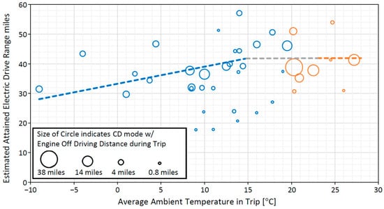 Figure 3. Scatter plot and piecewise linear regression fit of the attained EDR for the sample of 3 PHEVs.
2.2. Utility Factor Modeling with Progressively Relaxed Assumptions
2.2.1. Notations and Overview
A notation adopted in this work to indicate idealization assumptions is to indicate the assumption via a superscript capitalized letter. With SAE J2841 standard [28] as the reference, the superscripts indicating its idealized assumptions corresponding to the four main categories of reasons for UF mismatch, as illustrated in Figure 2, are as follows:
- Superscript of capitalized letter ‘D’ corresponds to the daily distance traveled by the vehicle being an exact match to the travel survey used for the SAE J2841 standard [28], which is the National Household Travel Survey of 2001 (NHTS-2001) [31].
- Superscript of capitalized letter ‘C’ corresponds to the charging behavior being an exact match to the assumption in SAE J2841 standard [28], which is that every driving day starts with a fully charged battery and no charging occurs during the day.
- Superscript of capitalized letter ‘R’ corresponds to the attained EDR being exactly the same as estimated by the vehicle’s EPA window-sticker label [36]. As a short notation, the symbol is also utilized to indicate the “rated EDR”.
- Superscript of capitalized letter ‘O’ corresponds to “no other effects”, and includes no blended operation in the real world if the PHEV did not experience any engine-on events in CD mode during the dynamometer tests for estimating its EDR.
The symbol is utilized to denote the fraction of distance traveled in CD mode with the engine off. From that, it follows that implies the real-world (no superscripts indicating idealization assumptions) total fraction traveled in CD mode with the engine off for a particular vehicle identified by the subscript. It follows that implies the fraction of distance traveled in CD mode with the engine off for an individual vehicle if “all” the idealization assumptions were met, which means that should be exactly equal to the standard UF curve value at an ordinal value of .
The core idea for the approach proposed in this work is that a “net UF mismatch” between and could be quantitatively categorized into individual contributions of the individual idealization assumptions via calculating “intermediate ” values with “some, but not all” of the superscripts/idealization assumptions. This will be further detailed in Section 2.2 and Section 2.3.
2.2.2. Relaxing the Assumption about Daily Distance Traveled
Calculating a partially theoretical UF value that corresponds to the real-world distance traveled while retaining all other idealization assumptions is fairly straightforward (it’s how one would generate a “real distance UF curve”, such as the one illustrated in Figure 2), but is re-capped using this paper’s adopted notations as follows:
where is the total distance traveled by a vehicle on a given day, while is the theoretical estimate for distance traveled in CD mode with the engine off under the idealization assumptions indicated in the superscript. The symbol , per the notations in Section 2.2.1, indicates the fraction of distance traveled in CD mode with the engine off by the vehicle sample ‘i’ if the charging (‘C’), attained EDR (‘R’), and other factors (‘O’) had occurred exactly as in the idealization assumptions in SAE J2841 standard.
2.2.3. Relaxing the Assumption about Charging Behavior
This subsection considers the calculation of a partially theoretical UF value after relaxing the assumption on the daily distance traveled while maintaining the assumption about EDR. This is conducted as follows:
where is the theoretical available electric driving distance at the beginning of a trip, assuming the EDR is perfectly attained and the charging behavior is that of the actual real-world vehicle in the dataset. This is calculated in Equation (4) by multiplying the relative SOC at the start of the trip (, from the actual vehicle data) by the rated EDR if it was the first trip of the day or if there was a detected charging event before the trip, with the charging event identification criteria being . For trips other than the first trip of a driving day and without a preceding charging event, the theoretical available electric driving distance is calculated as the available electric driving distance at the beginning of the last trip that had a charging event (denoted by ) minus the sum of total trip distances since the last charging event, or zero if the sum of the trip distances before the current trip exceeded the theoretical electric driving distance at the end of last charging event. , per Equation (5), is the expected electric distance traveled within a trip given ; then Equations (6) and (7) perform summations to calculate .
2.2.4. Relaxing the Assumption about Electric Driving Range
This subsection considers the calculation of a partially theoretical UF value after relaxing the assumption on the daily distance traveled while maintaining the assumption about charging behavior. In other words, assuming the vehicle starts with a fully charged battery at the beginning of every drive day but considering the impact of real-world driving conditions on the attained EDR. This is conducted as follows:
where is the theoretical estimate for the relative SOC available at the beginning of a trip. This is set to a value of 1.0 in Equation (8) per the charging assumption of a 100% full battery for the first trip of every drive day, and is then reduced by the estimated fraction of battery used (ratio of trip distance to attainable range ) in each trip from the start of the day until before the current trip. To avoid overly complex expressions in the calculation of , the symbol is introduced in Equations (10)–(12). The symbol denotes the estimated distance traveled in CD mode with the engine off (hence, it takes the minimum value of either the available range or trip distance in Equation (8)) while withholding the idealization assumptions of charging (‘C’) and other factors (‘O’). Both Equations (8) and (9) utilize the trip-specific attained EDR (), which, in turn, is estimated from the real-world trip rate of drop in SOC versus the distance traveled due to the effects of real-world driving conditions. However, when a direct estimate of is unavailable, the proxy estimate is utilized in Equations (8) and (9) instead.
2.2.5. Relaxing the Assumptions about Charging and Electric Driving Range
By combining the partially theoretical estimation approaches of Section 2.2.3 and Section 2.2.4, one may drive another partially theoretical estimate that relaxes all assumptions, except for the “Other” category of reasons for UF mismatch. This is conducted as follows:
where is the relative SOC (from the real-world trip data) at the beginning of a trip preceded by a charging event, or the first trip on a drive day.
2.3. Contributions of Real-World Factors
In addition to the partially theoretical values discussed in Section 2.2.2, Section 2.2.3, Section 2.2.4 and Section 2.2.5, one may utilize the real-world trips dataset to calculate, without any idealization assumptions, the real-world fraction of distance traveled in CD mode with the engine off (), as well as the fraction of distance traveled in all CD mode () for each vehicle as follows:
Furthermore, for a combination of relaxed idealization assumptions, it is possible to calculate a simple average (, analogous to MDIUF) or distance-weighted average (, analogous to FUF), where XX in the superscript indicates the combination of idealization assumptions that have been maintained, as follows:
The only exception to combinations of idealization assumptions where alternative calculations of and are utilized (aside from Equations (20) and (21)), is when all idealization assumptions are maintained, in which case, is equal to the standard MDIUF curve value at an ordinal value of , and is equal to the standard FUF curve value at an ordinal value of , or when none of the idealization assumptions are maintained, which implies the real-world UF from the dataset, which according to the definition in the SAE J2841 standard [28], should include all of the CD mode, thus, replaces in Equations (20) and (21) as follows:
UF mismatch indices () are then proposed as a means of quantification of a particular category of real-world factors as the ratio of a quantity with fewer idealization assumptions to a quantity with more idealization assumptions. As a notation, superscripts for the UF mismatch indices indicate the idealization assumption whose effect is being isolated/quantified. Mismatch indices may be calculated for individual vehicle samples, in which case, a subscript indicating the vehicle sample will be included, or the indices can be calculated for the whole dataset. When considering the whole dataset of vehicle samples, mismatch indices may be used to quantify the mismatch in MDIUF, in which case, ratios of from Equation (20) will be used, or to quantify the mismatch in FUF, which the rest of this paper focuses on, for-which ratios of will be used. With these notations, the FUF mismatch index quantifying the effect of daily distance traveled is expressed as follows:
Furthermore, the FUF mismatch index quantifying the effect of charging behavior, if one considers isolating the effect of charging behavior before that of attained EDR, could be expressed as follows:
Alternatively, if one considers isolating the effect of the attained EDR first, then the “follow-up” FUF mismatch index quantifying the effect of charging behavior would be expressed as follows:
where the ‘~’ marker above the -symbol in Equation (26) signifies an alternative value for the real-world factor being isolated. More specifically, in this work, ‘~’ indicates that the contribution of the real-world factor is estimated at a later stage, rather than earlier.
Similar to Equations (25) and (26), the FUF mismatch index quantifying the effect of the attained EDR, depending on whether the effect of charging behavior is isolated first or not, is expressed as follows:
Lastly, the FUF mismatch index quantifying the effect of “all other reasons” is expressed as follows:
3. Results and Discussion
Applying the approach discussed in Section 2.2 and Section 2.3 to the trip-level data discussed in Section 2.1 (also fully listed in Table A1 in Appendix A), UF with progressively relaxed idealization assumptions at the vehicle-level and fleet-level (weighted average by vehicle distance traveled) are summarized in Table 3. UF mismatch indices corresponding to the contributions of all four categories of reasons for mismatch between a standard UF curve (using SAE J2841 FUF as the reference) and the real world are also summarized in Table 3 and Figure 4. Table 3 lists key quantities of interest for each of the three individual vehicles, as well as at the “Fleet” level. For total driving distance, the “fleet” value in Table 3 is simply the sum of the total driving distances of all three vehicles. For all other quantities in Table 3 (UF, fraction of distance traveled in CD mode with engine off, and UF mismatch indices), the “fleet” value is the distance-weighted average among the three vehicles.
Table 3.
Utility Factor results at the vehicle and fleet levels.
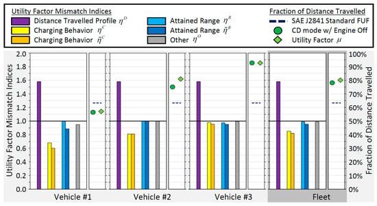
Figure 4.
UF mismatch indices and fraction of the distance traveled at the vehicle and fleet levels.
It is noted that, by construction, the UF mismatch indices are rational numbers that signify whether the real-world usage of a PHEV in one category of reasons is better (index value greater than 1.0), worse (index value less than 1.0) or not significantly different (index value close to 1.0) than the corresponding idealization assumption in the standard. It is also true (by construction) that sequentially multiplying the UF mismatch indices provides a mapping between the standard UF value to the real-world observed one, thus, both Equations (30) and (31), as follows, hold true:
where is the standard UF curve value at an ordinal equal to the rated EDR.
One observation from Figure 4 is that the UF mismatch index corresponding to the distance traveled is significantly greater than 1.0 for all three vehicles. In fact, due to the nature of the relatively short data collection period, where no long-distance trips occurred, and the travel distance on any day did not exceed the rated EDR, if everything else was in accordance with the standard idealization assumptions, then each vehicle should have been able to attain a UF value of 100% based on daily travel distance alone. However, when factoring in the other categories of reasons for UF mismatch, vehicle no. 1 (which had the most “less than ideal” charging pattern) ended up having less UF than the standard UF (marked by a dashed dark blue line in right-side mini plot within Figure 4), while vehicle nos. 2 and 3, as well as the fleet-level (each vehicle weighted by its total travel distance), were better than the standard UF. Although results with such a small sample of vehicles and trips are not population-representative, they serve to demonstrate the proposed approach. The computational burden of the proposed approach (Equations (1)–(29)) is proportional to the data size (number of vehicles and number of trips per vehicle), with no higher-order (O(N2)) computations; thus, the computations should be easily scalable to large datasets.
Another observation from Figure 4 is that the “Other” category (gray-colored bar plot in Figure 4), which is the “catch-all” for things not accounted for in the modeling, does not appear to be significant for vehicle nos. 2 and 3, and only has a small contribution in vehicle no. 1, which also happened to be the vehicle that was driven in the coldest climate conditions. Although the climate effect is meant to be accounted for as part of the attained EDR category, the effects of certain real-world factors, such as the drop in battery SOC while the vehicle is not driving (i.e., in between trips, as sometimes observed in Table A1), are part of the “Other reasons” category.
One possible limitation of the proposed approach is its sequential nature of estimating the contributions of the various idealization assumptions toward UF mismatch “one at a time”, when in fact they can be “intertwined”, as shown for vehicle no. 1 in Figure 4. This complex interaction between real-world factors can lead to differences in the results of the mismatch index of UF charging behavior (yellow/orange bar plots in Figure 4) and the mismatch index of UF for attained EDR (blue-toned plots in Figure 4), depending on the order of which category was analyzed first.
Assume a hypothetical scenario, where an owner of a PHEV with a rated EDR of 50 miles ends one driving day with a battery SOC at 80% of its range (thus, it seems like 40 miles of electric driving is still available), and the owner knows that the next day would only involve 40 miles of travel distance. Then, the vehicle owner, thinking they had sufficient available range, decides not to charge overnight. However, the attained EDR in the hypothetical scenario for the next day is 48 miles (instead of the rated 50 miles), 80% of which is 38.4 miles, which is less than the 40-mile travel distance for the day. Even ignoring the SOC drop while the vehicle is parked, in this scenario, one may consider the following paradoxical question: “Is the reason they couldn’t complete that drive day as all-electric due to charging behavior or due to attained EDR?” On one hand, if the owner had charged to full overnight, the drive day in question would have been all-electric driving despite the attained EDR being imperfect. But on the other hand, if the driving conditions had enabled attaining the rated EDR, then the drive day in question would have been all-electric driving despite the charging behavior being imperfect. In the authors’ opinion, the answer to the paradoxical question in the hypothetical scenario involves neither charging nor attaining EDR on its own, but the combined interaction between both.
Dependance on the order of relaxing the idealization assumptions via the proposed approach was visibly pronounced in one out of three sample vehicles in the current work, but how much of a difference could occur, the application to a larger sample of vehicles, as well as extending the derivations in this paper to simultaneous quantification (rather than sequential) are interesting research issues that could be pursued in future work. While noting such limitations, the proposed approach has advantages in its computational scalability that allow it to be readily applied to large datasets to detangle and estimate the contributions of different reasons for UF mismatch at fleet-representative scales. In recent years, there has been increased interest in revisions to UF curves to better match the perceived real-world performance of PHEVs [41]. Unfortunately, assessments in [41] have relied on literature publications that exhibited errors (such as [23], which was later corrected in [26]) and have not attempted to discern the contributions of different reasons for why PHEVs might not meet the UF standard. While acknowledging that revisions of UF standards are complex tasks, the approach proposed in this work may offer ways to gain better insights that would be beneficial when developing future UF standards.
4. Conclusions
This paper proposes an approach to quantitatively assess the contributions of various categories of reasons for mismatch between standard UF curves and those observed in the real world for PHEVs. The approach relies on progressively relaxing the idealization assumptions that had been made in the development of standard UF. By relaxing one idealization assumption at a time and comparing a “more ideal” to a “less ideal” UF estimate, one can quantify the contribution of that one idealization assumption. Generation of results via the proposed approach was demonstrated via real-world trip-level data from three PHEVs that have been each monitored for a period of one week. The observed results hint that any/all reasons for UF mismatch could be of significance. However, the small data sample size, both in terms of the number of vehicles, as well as the duration of monitoring, cannot be utilized to draw population-representative conclusions. An advantage of the proposed approach is that the computational burden is proportional to the sample size of the data, with no higher-order terms, and should be readily scalable to larger datasets. Observation of the results also calls into question the complex nature of interactions between categories of reasons for UF mismatch, where results of the proposed approach may be affected to some extent by the order of relaxing the UF idealization assumptions. Such complexities, as well as the application of the proposed approach to larger datasets, may be considered in future work.
Author Contributions
Conceptualization, K.H. and K.L.; methodology, K.H.; software, K.H.; validation, K.H., K.L., and K.-C.C.; formal analysis, K.H., K.L., and K.-C.C.; data curation, K.L. and K.-C.C.; writing—original draft preparation, K.H.; writing—review and editing, K.L. and K.-C.C.; visualization, K.H. and K.-C.C.; supervision, K.L.; project administration, K.L.; funding acquisition, K.L. All authors have read and agreed to the published version of the manuscript.
Funding
This research received no external funding.
Data Availability Statement
Vehicle trip-level data that enables the regeneration of results in this paper are included in Appendix A.
Conflicts of Interest
Kang-Ching Chu has no conflicts of interest to declare. Karim Hamza and Kenneth Laberteaux are employees of Toyota Motor North America. This paper reflects their views as scientists and not the views of the company.
Acronyms
| BEV | battery-only electric vehicle |
| CD | charge depletion |
| CICE | conventional internal combustion engine |
| CS | charge-sustaining |
| EDR | electric driving range |
| EU | European Union |
| FC | fuel cell |
| FCEV | fuel cell electric vehicle |
| FUF | fleet utility factor |
| GHG | greenhouse gas |
| HEV | hybrid electric vehicle |
| ICE | internal combustion engine |
| MDIUF | multi-day individual utility factor |
| NEDC | New European Drive Cycle (utilized in the EU before the adoption of WLTP) |
| NHTS | National Household Travel Survey |
| OBD | on-board diagnostics |
| PFCEV | plug-in fuel cell electric vehicle |
| PHEV | plug-in hybrid electric vehicle |
| SAE | Society of Automotive Engineers |
| SOC | state of charge |
| UF | utility factor |
| WLTP | Worldwide Harmonized Light Vehicle Test Procedure |
Appendix A
Table A1.
Trip-level summaries of the data collected from real-world PHEVs.
Table A1.
Trip-level summaries of the data collected from real-world PHEVs.
| Vehicle | Drive Day | Trip of Day | Trip Data | |||||||
|---|---|---|---|---|---|---|---|---|---|---|
| 1 | 1 | 1 | 14.199 | 0.5% | 0.0% | 3.7 | 35.4 | 0.000 | 0.000 | |
| 1 | 2 | 1 | 10.977 | 11.3% | 0.0% | 3.7 | 34.4 | 3.882 | 0.000 | |
| 1 | 3 | 1 | 5.029 | 100.0% | 89.2% | 4.4 | 46.7 | 5.029 | 0.000 | |
| 1 | 3 | 2 | 3.078 | 87.7% | 78.0% | 2.0 | 36.6 | 3.078 | 0.000 | |
| 1 | 3 | 3 | 5.944 | 69.8% | 49.8% | 1.0 | 29.7 | 5.944 | 0.000 | |
| 1 | 4 | 1 | 7.370 | 46.2% | 26.2% | 8.5 | 32.0 | 6.894 | 0.500 | |
| 1 | 4 | 2 | 2.112 | 17.4% | 10.8% | 8.5 | 31.7 | 2.112 | 0.000 | |
| 1 | 4 | 3 | 6.129 | 10.3% | 0.0% | 9.7 | 31.9 | 3.280 | 0.000 | |
| 1 | 4 | 4 | 6.253 | 0.0% | 0.0% | 9.3 | 38.7 | 0.000 | 0.000 | |
| 1 | 5 | 1 | 4.064 | 99.5% | 89.8% | −4.0 | 43.4 | 4.064 | 0.000 | |
| 1 | 5 | 2 | 5.498 | 74.9% | 57.4% | −9.0 | 31.5 | 5.498 | 0.000 | |
| 2 | 1 | 1 | 9.918 | 0.0% | 0.0% | 21.5 | 42.0 | 0.000 | 0.000 | |
| 2 | 1 | 2 | 3.387 | 0.0% | 1.0% | 21.5 | 42.0 | 0.013 | 0.000 | |
| 2 | 1 | 3 | 3.328 | 1.0% | 0.0% | 20.7 | 42.0 | 0.000 | 0.000 | |
| 2 | 2 | 1 | 7.327 | 100.0% | 85.1% | 20.2 | 51.0 | 7.327 | 0.000 | |
| 2 | 3 | 1 | 6.206 | 94.9% | 81.5% | 16.0 | 46.5 | 6.206 | 0.000 | |
| 2 | 3 | 2 | 4.408 | 80.5% | 71.8% | 17.8 | 50.6 | 4.408 | 0.000 | |
| 2 | 3 | 3 | 4.226 | 71.8% | 61.0% | 14.4 | 39.2 | 4.226 | 0.000 | |
| 2 | 3 | 4 | 4.098 | 59.5% | 52.3% | 14.0 | 57.1 | 4.098 | 0.000 | |
| 2 | 3 | 5 | 3.901 | 52.3% | 42.6% | 12.9 | 40.0 | 3.901 | 0.000 | |
| 2 | 4 | 1 | 11.473 | 99.5% | 73.9% | 12.5 | 39.2 | 9.257 | 2.200 | |
| 2 | 4 | 2 | 11.762 | 97.4% | 67.7% | 8.3 | 37.7 | 10.451 | 1.300 | |
| 2 | 5 | 1 | 2.960 | 65.7% | 59.0% | 14.0 | 44.4 | 2.960 | 0.000 | |
| 2 | 5 | 2 | 1.591 | 56.4% | 52.8% | 13.5 | 44.3 | 1.591 | 0.000 | |
| 2 | 5 | 3 | 1.337 | 53.3% | 49.8% | 13.9 | 37.2 | 1.337 | 0.000 | |
| 2 | 6 | 1 | 11.023 | 50.8% | 23.1% | 20.9 | 35.2 | 9.377 | 1.600 | |
| 3 | 1 | 1 | 16.482 | 100.0% | 56.4% | 22.5 | 37.8 | 16.482 | 0.000 | |
| 3 | 1 | 2 | 1.732 | 53.3% | 47.7% | 20.3 | 30.7 | 1.732 | 0.000 | |
| 3 | 1 | 3 | 0.768 | 48.2% | 46.2% | 19.0 | 37.4 | 0.768 | 0.000 | |
| 3 | 1 | 4 | 0.973 | 46.2% | 42.6% | 17.8 | 27.1 | 0.973 | 0.000 | |
| 3 | 2 | 1 | 1.793 | 42.1% | 36.4% | 11.0 | 31.8 | 1.793 | 0.000 | |
| 3 | 2 | 2 | 1.843 | 35.4% | 27.7% | 13.4 | 24.0 | 1.843 | 0.000 | |
| 3 | 2 | 3 | 16.771 | 27.7% | 1.0% | 19.5 | 46.1 | 12.766 | 0.000 | |
| 3 | 2 | 4 | 0.101 | 1.0% | 0.5% | 21.0 | 42.0 | 0.005 | 0.000 | |
| 3 | 2 | 5 | 0.044 | 0.5% | 0.5% | 21.0 | 42.0 | 0.000 | 0.000 | |
| 3 | 2 | 6 | 1.661 | 93.9% | 90.8% | 24.7 | 54.0 | 1.661 | 0.000 | |
| 3 | 2 | 7 | 16.08 | 100.0% | 61.0% | 27.2 | 41.3 | 16.080 | 0.000 | |
| 3 | 2 | 8 | 0.954 | 56.9% | 53.9% | 26.0 | 31.0 | 0.954 | 0.000 | |
| 3 | 2 | 9 | 0.847 | 53.9% | 51.8% | 24.5 | 41.3 | 0.847 | 0.000 | |
| 3 | 3 | 1 | 0.385 | 49.8% | 48.7% | 12.0 | 40.2 | 0.385 | 0.000 | |
| 3 | 3 | 2 | 0.853 | 41.0% | 37.4% | 9.9 | 23.8 | 0.853 | 0.000 | |
| 3 | 3 | 3 | 0.817 | 37.4% | 32.8% | 9.0 | 17.7 | 0.817 | 0.000 | |
| 3 | 4 | 1 | 0.789 | 44.6% | 43.1% | 11.6 | 51.3 | 0.789 | 0.000 | |
| 3 | 4 | 2 | 0.911 | 42.6% | 37.4% | 11.0 | 17.8 | 0.911 | 0.000 | |
| 3 | 5 | 1 | 15.924 | 38.0% | 0.5% | 10.0 | 36.5 | 13.860 | 0.000 | |
| 3 | 6 | 1 | 0.741 | 100.0% | 96.4% | 13.8 | 20.7 | 0.741 | 0.000 | |
| 3 | 6 | 2 | 0.351 | 96.4% | 93.9% | 10.0 | 39.1 | 0.351 | 0.000 | |
| 3 | 6 | 3 | 0.844 | 92.8% | 89.2% | 16.0 | 23.5 | 0.844 | 0.000 | |
| 3 | 7 | 1 | 41.787 | 100.0% | 0.0% | 20.3 | 38.8 | 38.849 | 0.000 | |
References
- US Department of Energy. Hybrid and Plug-in Electric Vehicles. Available online: https://www.energy.gov/sites/prod/files/2014/05/f15/52723.pdf (accessed on 28 August 2024).
- US Energy Information Administration. Today in Energy. Available online: https://www.eia.gov/todayinenergy/detail.php?id=36312 (accessed on 28 August 2024).
- US Department of Energy. Fuel Cell Electric Vehicles. Available online: https://afdc.energy.gov/vehicles/fuel-cell (accessed on 28 August 2024).
- Yuksel, T.; Michalek, J. Effects of Regional Temperature on Electric Vehicle Efficiency, Range, and Emissions in the United States. Environ. Sci. Technol. 2015, 49, 3974–3980. [Google Scholar] [CrossRef] [PubMed]
- Yuksel, T.; Tamayao, A.M.; Hendrickson, C.; Azevedo, I.M.L.; Michalek, J. Effect of regional grid mix, driving patterns and climate on the comparative carbon footprint of gasoline and plug-in electric vehicles in the United States. Environ. Res. Lett. 2016, 11, 044007. [Google Scholar] [CrossRef]
- Our World in Data. Carbon Intensity of Electricity Generation. Available online: https://ourworldindata.org/grapher/carbon-intensity-electricity (accessed on 28 August 2024).
- Helveston, J.P.; Liu, Y.; Feit, E.M.; Fuchs, E.; Klampfl, E.; Michalek, J. Will subsidies drive electric vehicle adoption? Measuring consumer preferences in the U.S. and China. Transp. Res. Part A 2015, 73, 96–112. [Google Scholar] [CrossRef]
- Shetty, D.; Shetty, S.; Rodrigues, L.R.; Naik, N.; Maddodi, C.B.; Malarout, N.; Sooriyaperakasam, N. Barriers to widespread adoption of plug-in electric vehicles in emerging Asian markets: An analysis of consumer behavioral attitudes and perceptions. Cogent Eng. 2020, 7, 1796198. [Google Scholar] [CrossRef]
- Krishna, G. Understanding and identifying barriers to electric vehicle adoption through thematic analysis. Transp. Res. Interdiscip. Perspect. 2021, 10, 100364. [Google Scholar] [CrossRef]
- Rajper, S.Z.; Albrecht, J. Prospects of Electric Vehicles in the Developing Countries: A Literature Review. Sustainability 2020, 12, 1906. [Google Scholar] [CrossRef]
- Hamza, K.; Laberteaux, K.; Chu, K.C. On Modeling the Total Cost of Ownership of Electric and Plug-in Hybrid Vehicles. SAE Tech. Pap. 2020, 2020-01-1435. [Google Scholar] [CrossRef]
- Liu, Z.; Song, J.; Kabul, J.; Susarla, N.; Knehr, K.W.; Islam, E.; Nelson, P.; Ahmed, S. Comparing total cost of ownership of battery electric vehicles and internal combustion engine vehicles. Energy Policy 2021, 158, 112564. [Google Scholar] [CrossRef]
- Sahfiei, E.; Dauphin, R.; Yugo, M. Optimal electrification level of passenger cars in Europe in a battery-constrained future. Transp. Res. Part D 2022, 102, 103132. [Google Scholar] [CrossRef]
- He, X.; Wang, F.; Wallington, T.J.; Shen, W.; Melaina, M.W.; Kim, H.C.; De Kleine, R.; Lin, T.; Zhang, S.; Keoleian, G.A.; et al. Well-to-wheels emissions, costs, and feedstock potentials for light-duty hydrogen fuel cell vehicles in China in 2017 and 2030. Renew. Sustain. Energy Rev. 2021, 137, 110477. [Google Scholar] [CrossRef]
- Kim, J.H.; Kim, H.J.; Yoo, S.H. Willingness to pay for fuel-cell electric vehicles in South Korea. Energy 2019, 174, 497–502. [Google Scholar] [CrossRef]
- Samaras, C.; Meisterling, K. Life Cycle Assessment of Greenhouse Gas Emissions from Plug-in Hybrid Vehicles: Implications for Policy. Environ. Sci. Technol. 2008, 42, 3170–3176. [Google Scholar] [CrossRef] [PubMed]
- Bradley, T.; Frank, A. Design, demonstrations and sustainability impact assessments for plug-in hybrid electric vehicles. Renew. Sustain. Energy Rev. 2009, 13, 115–128. [Google Scholar] [CrossRef]
- Patil, R.; Adoranto, B.; Filipi, Z. Design Optimization of a Series Plug-In Hybrid Electric Vehicle for Real-World Driving Conditions. SAE Int. J. Engines 2010, 3, 655–665. [Google Scholar] [CrossRef][Green Version]
- Raykin, L.; Roorda, M.; MacLean, H. Impacts of driving patterns on tank-to-wheel energy use of plug-in hybrid electric vehicles. Transp. Res. Part D 2012, 17, 243–250. [Google Scholar] [CrossRef]
- Karabasoglu, O.; Michalek, J. Influence of driving patterns on life cycle cost and emissions of hybrid and plug-in electric vehicle power trains. Energy Policy 2013, 60, 445–461. [Google Scholar] [CrossRef]
- Plötz, P.; Jakobsson, N.; Sprei, F. On the distribution of individual daily driving distances. Transp. Res. Part B 2017, 101, 213–227. [Google Scholar] [CrossRef]
- Laberteaux, K.; Hamza, K.; Willard, J. Optimizing the electric range of plug-in vehicles via fuel economy simulations of real-world driving in California. Transp. Res. Part D 2019, 73, 15–33. [Google Scholar] [CrossRef]
- Plötz, P.; Moll, C.; Bieker, G.; Mock, P. From lab-to-road: Real-world fuel consumption and CO2 emissions of plug-in hybrid electric vehicles. Environ. Res. Lett. 2021, 16, 054078. [Google Scholar] [CrossRef]
- Isenstadt, A.; Yang, Z.; Searle, S.; German, J. Real World Usage of Plug-in Hybrid Vehicles in the United States. ICCT White Paper. 2022. Available online: https://theicct.org/wp-content/uploads/2022/12/real-world-phev-us-dec22.pdf (accessed on 30 December 2022).
- Hamza, K.; Laberteaux, K.; Chu, K.C. On inferred real-world fuel consumption of past decade plug-in hybrid electric vehicles in the US. Environ. Res. Lett. 2022, 17, 104053. [Google Scholar] [CrossRef]
- Plötz, P.; Moll, C.; Bieker, G.; Mock, P. Corrigendum: From lab-to-road: Real-world fuel consumption and CO2 emissions of plug-in hybrid electric vehicles (2021 Environ. Res. Lett. 16 054078). Environ. Res. Lett. 2023, 18, 099502. [Google Scholar] [CrossRef]
- Hamza, K.; Laberteaux, K. On the Need for Revisions of Utility Factor Curves for Plug-In Hybrids in the US. SAE Tech. Pap. 2024, 2024-01-2155. [Google Scholar] [CrossRef]
- Society of Automotive Engineers. Utility Factor Definitions for Plug-In Hybrid Electric Vehicles Using Travel Survey Data. 2010. Available online: https://www.sae.org/standards/content/j2841_201009/ (accessed on 28 August 2024).
- Wikipedia. New European Driving Cycle. Available online: https://en.wikipedia.org/wiki/New_European_Driving_Cycle (accessed on 28 August 2024).
- Plötz, P.; Moll, C.; Bieker, G.; Mock, P.; Li, Y. Real-World Usage of Plug-in Hybrid Electric Vehicles Fuel Consumption Electric Driving and CO2 Emissions. ICCT White Paper 2020. Available online: https://theicct.org/wp-content/uploads/2021/06/PHEV-white-paper-sept2020-0.pdf (accessed on 28 August 2024).
- US Department of Transportation. National Household Travel Survey. 2001. Available online: https://nhts.ornl.gov/download.shtml#2001 (accessed on 30 May 2022).
- European Commission. Technical Report on the Development of a Worldwide Harmonised Light Duty Vehicle Test Procedure (WLTP). UN/ECE/WP.29/GRPE/WLTP-IG. 2015. Available online: https://unece.org/fileadmin/DAM/trans/doc/2015/wp29grpe/GRPE-72-02.pdf (accessed on 28 August 2024).
- Raghavan, S.S.; Tal, G. Influence of User Preferences on the Revealed Utility Factor of Plug-In Hybrid Electric Vehicles. World Electr. Veh. J. 2020, 11, 6. [Google Scholar] [CrossRef]
- Raghavan, S.S.; Tal, G. Plug-in hybrid electric vehicle observed utility factor: Why the observed electrification performance differ from expectations. Int. J. Sustain. Transp. 2022, 16, 10–136. [Google Scholar] [CrossRef]
- Hamza, K.; Laberteaux, K. Utility Factor Curves for Plug-in Hybrid Electric Vehicles: Beyond the Standard Assumptions. World Electr. Veh. J. 2023, 14, 301. [Google Scholar] [CrossRef]
- US Department of Energy. Compare Side by Side. Available online: https://www.fueleconomy.gov/feg/Find.do?action=sbs&id=42793 (accessed on 28 August 2024).
- OBDLink. OBDLINK MX+. Available online: https://www.obdlink.com/products/obdlink-mxp/ (accessed on 28 August 2024).
- Wu, D.; Guo, F.; Field, F.R.; De Kleine, R.D.; Kim, H.C.; Wallington, T.J.; Kirchain, R.E. Regional Heterogeneity in the Emissions Benefits of Electrified and Lightweighted Light-Duty Vehicles. Environ. Sci. Technol. 2019, 53, 10560–10570. [Google Scholar] [CrossRef]
- Henrique, D.B. Evaluating the Energy Consumption of Battery Electric Vehicles Under a Diverse and Changing Climate. Master’s Thesis, University of Toronto, Toronto, ON, Canada, 2021. Available online: https://tspace.library.utoronto.ca/handle/1807/125841 (accessed on 28 August 2024).
- Sørensen, A.L.; Ludvigsen, B.; Andresen, I. Grid-connected cabin preheating of Electric Vehicles in cold climates—A non-flexible share of the EV energy use. Appl. Energy 2023, 341, 121054. [Google Scholar] [CrossRef]
- US Environmental Protection Agency. Multi-Pollutant Emissions Standards for Model Years 2027 and Later Light-Duty and Medi-um-Duty Vehicles. 2023. Available online: https://www.regulations.gov/search?documentTypes=Proposed%20Rule&filter=EPA-HQ-OAR-2022-0829 (accessed on 1 September 2024).


Disclaimer/Publisher’s Note: The statements, opinions and data contained in all publications are solely those of the individual author(s) and contributor(s) and not of MDPI and/or the editor(s). MDPI and/or the editor(s) disclaim responsibility for any injury to people or property resulting from any ideas, methods, instructions or products referred to in the content. |
© 2024 by the authors. Published by MDPI on behalf of the World Electric Vehicle Association. Licensee MDPI, Basel, Switzerland. This article is an open access article distributed under the terms and conditions of the Creative Commons Attribution (CC BY) license (https://creativecommons.org/licenses/by/4.0/).