
Power Optimization of Multi-Type Mixed-Connection Photovoltaic Generation System for Recreational Vehicles


Abstract
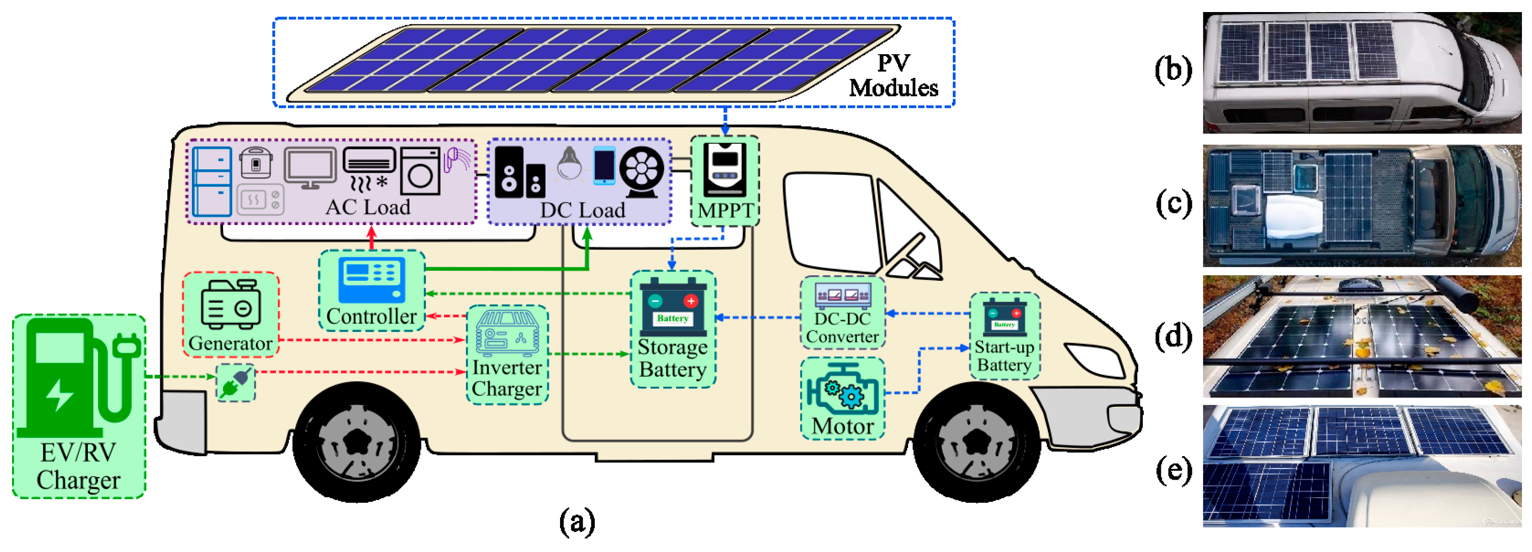
:1. Introduction
2. Characteristics of PV Modules and Methods for Configuring Multiple Types of PV Module Systems
2.1. Characteristics of Solar Cells and PV Modules
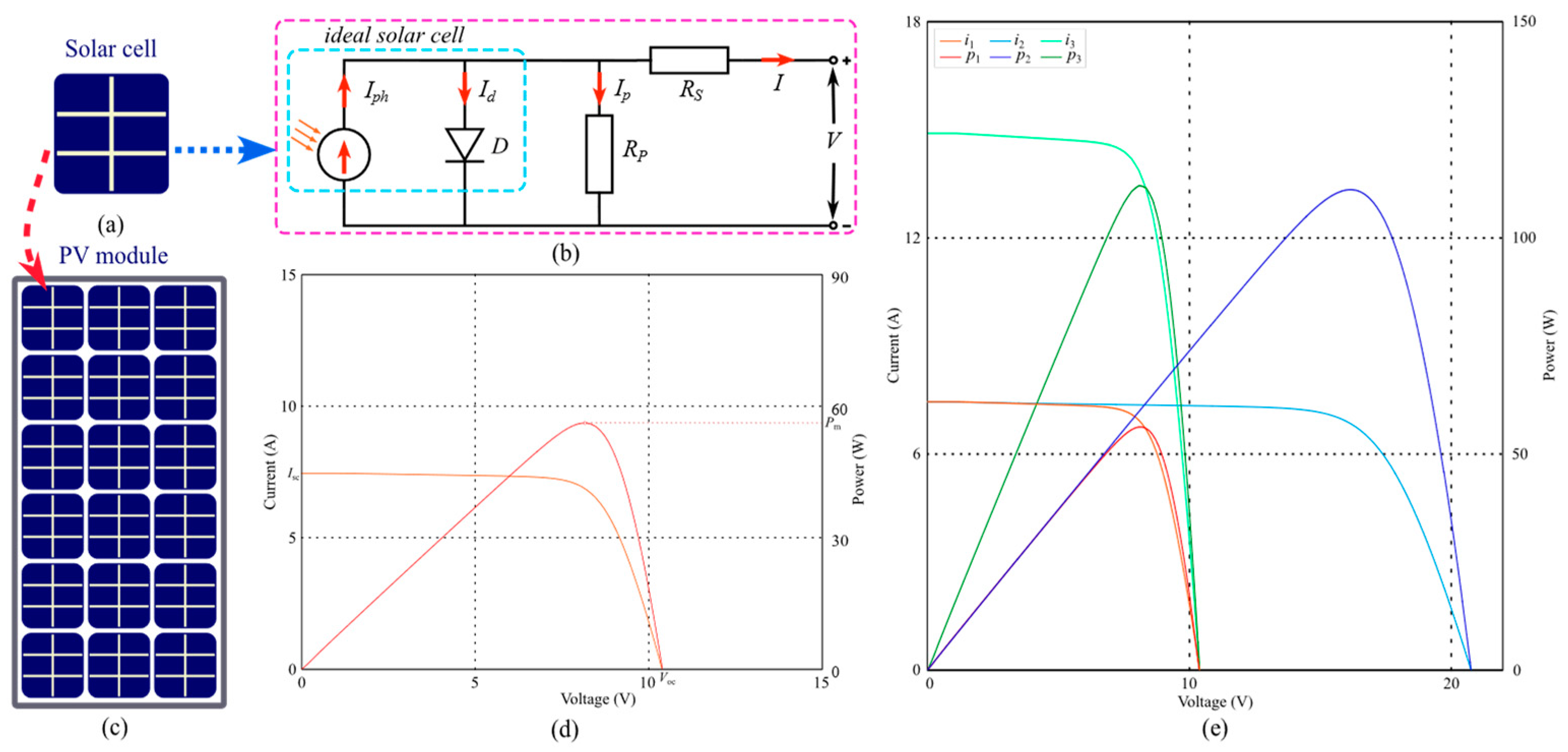
- Iph: current generated by incident light;
- I0: reverse saturation or leakage current of diode;
- q: electron charge (1.60217646 × 10⁻¹⁹ C);
- k: Boltzmann constant (1.3806503 × 10⁻²³ J/K);
- T: temperature of the p–n junction (in Kelvin);
- α: diode ideality constant.
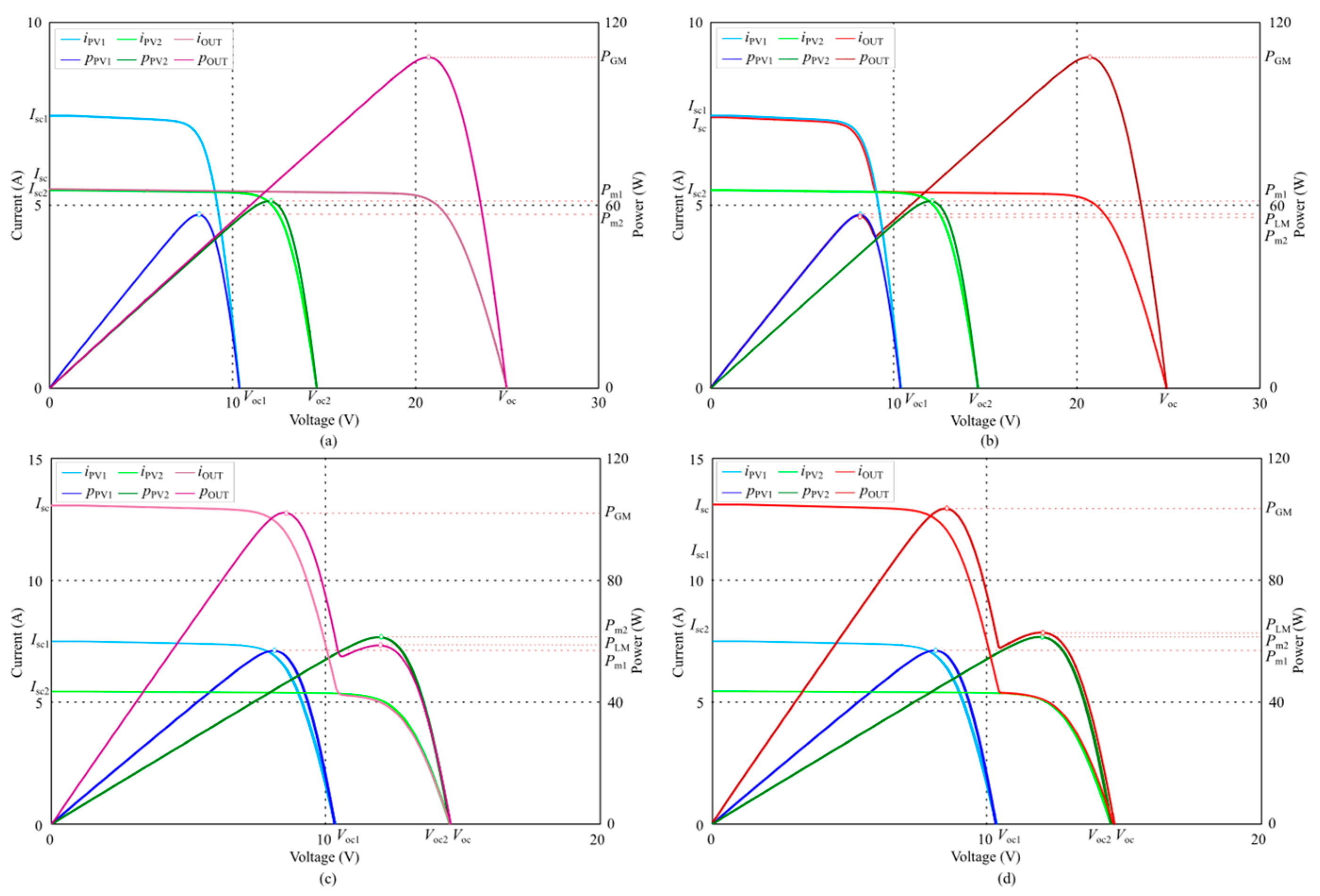
2.2. Output Characteristics of Different Types of PV Modules in Series or Parallel
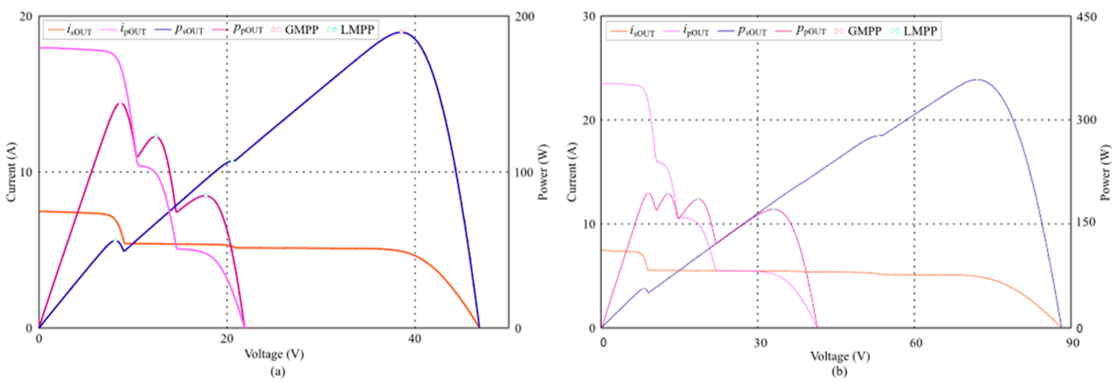
2.3. Method of Configuring PV modules in Multi-Type Mixed Connection System
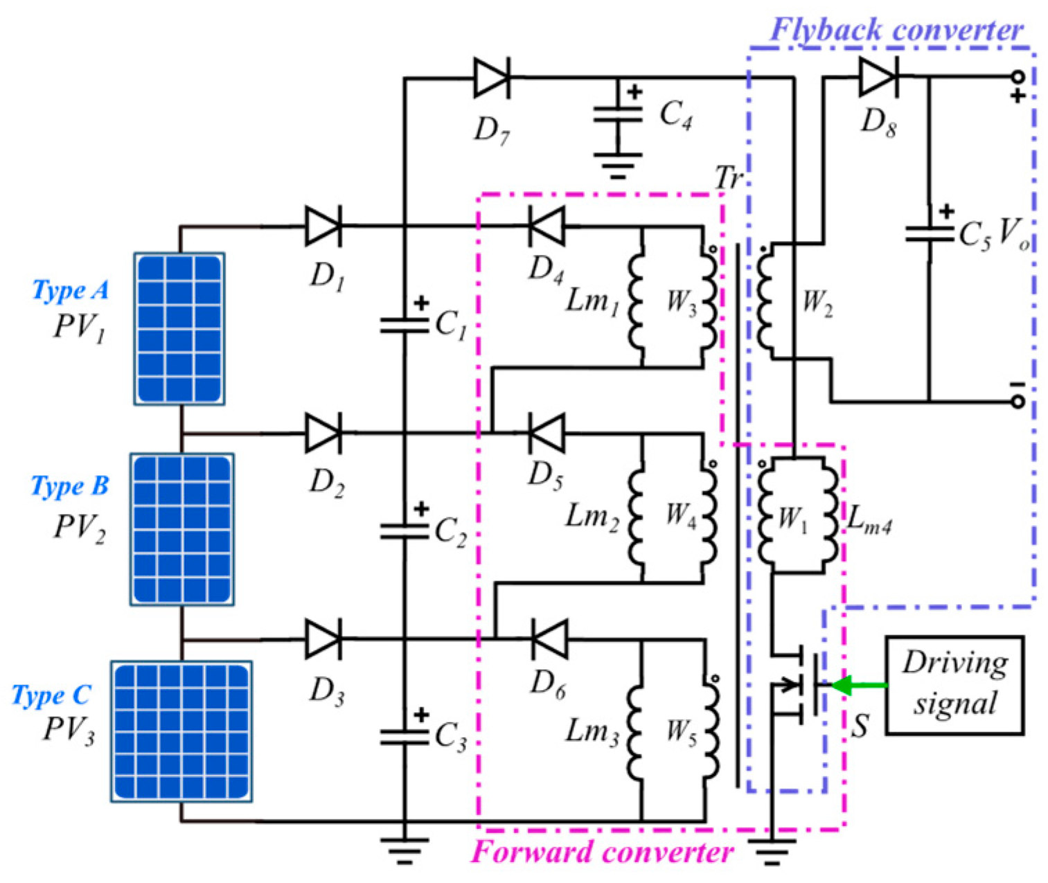
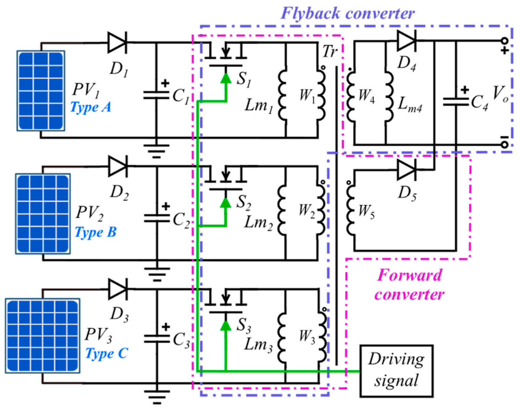
3. Forward–Flyback Converter-Based Equalizer
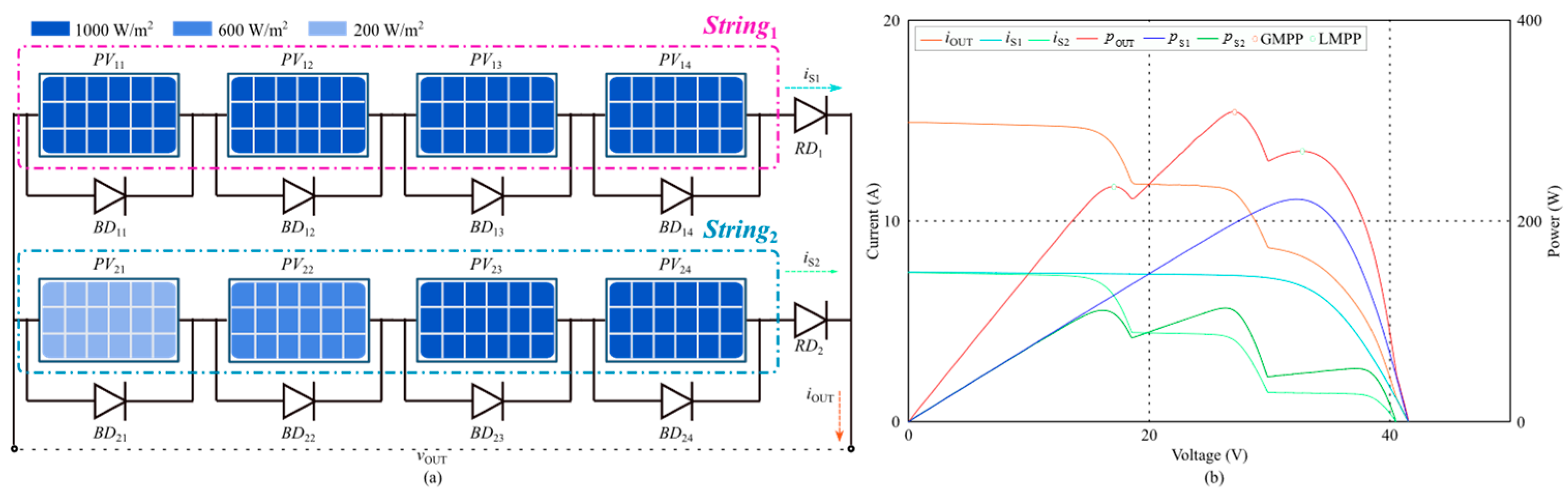
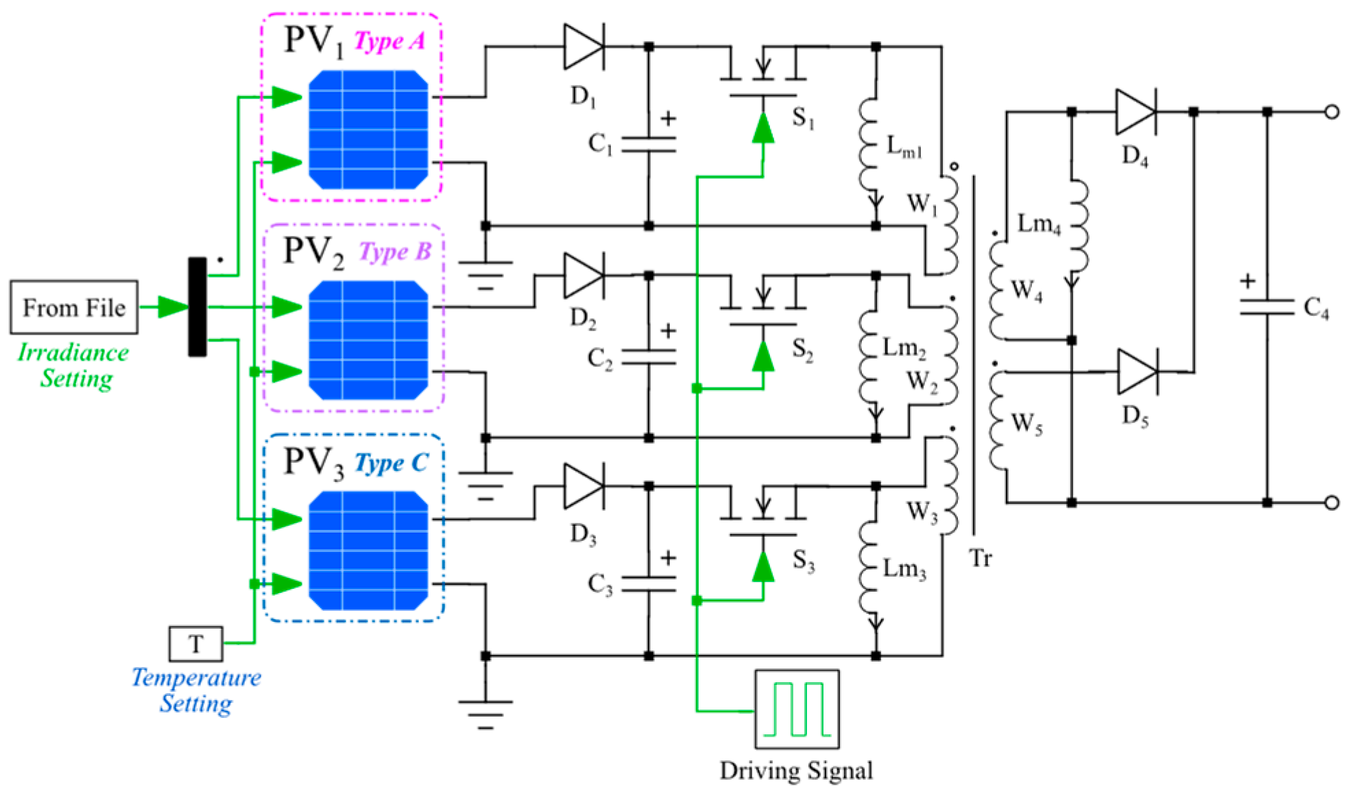
3.1. Current Equalization for Series-Connected PV Modules
3.2. Voltage Matching for Parallel-Connected PV Modules
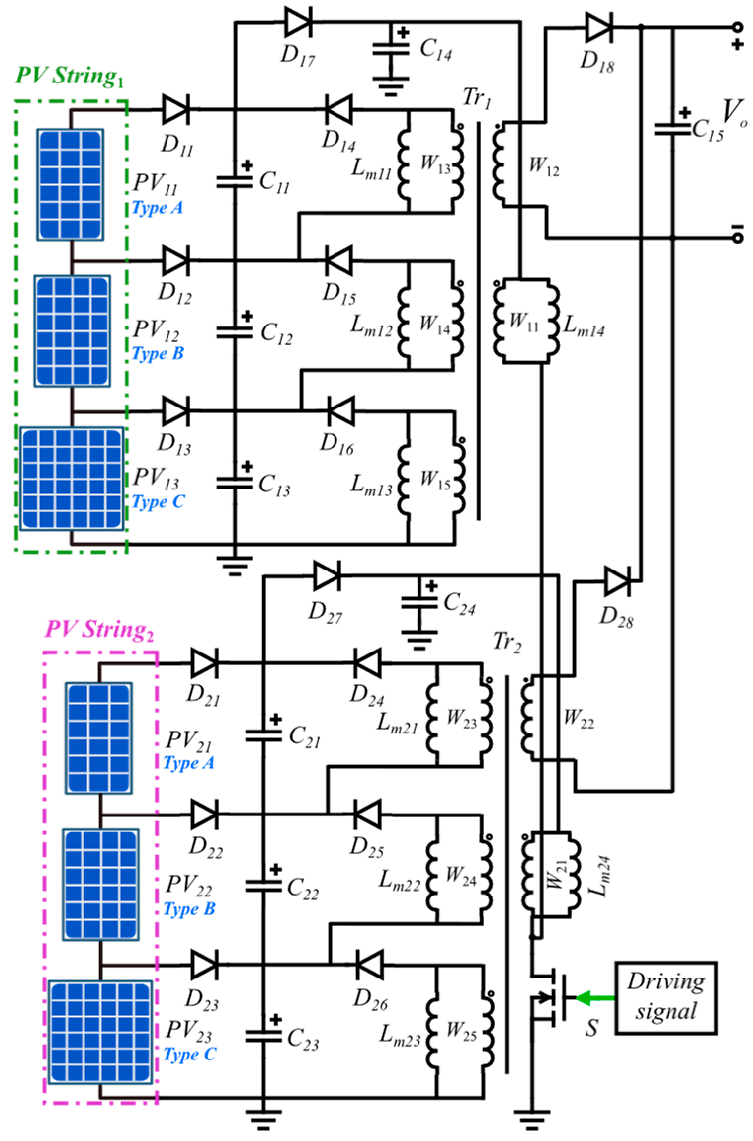
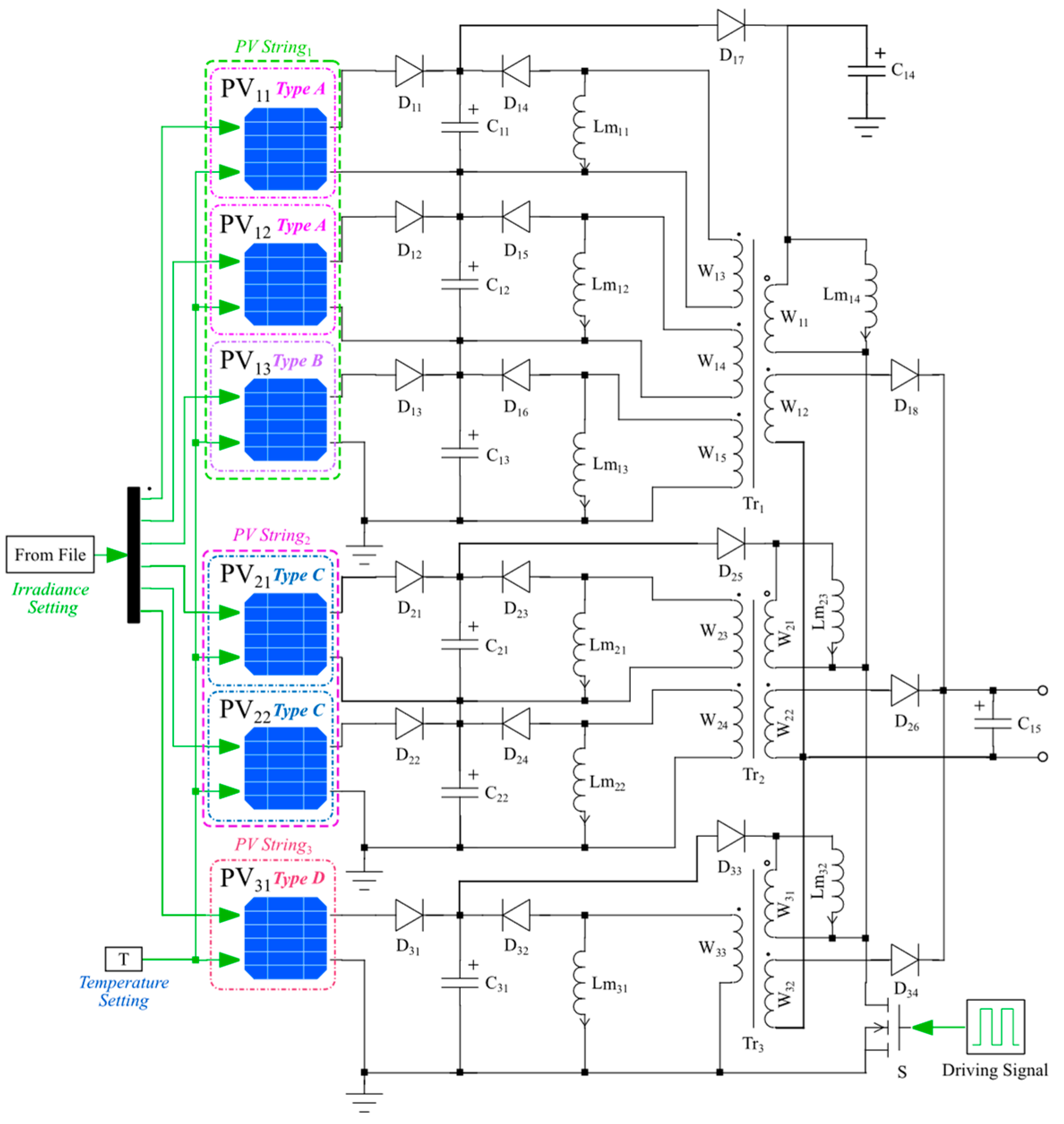
3.3. Power Equalization for Mixed Series–Parallel-Connected PV Modules
4. Maximum Power Acquisition of PV Generation System Based on Extremum-Seeking Control
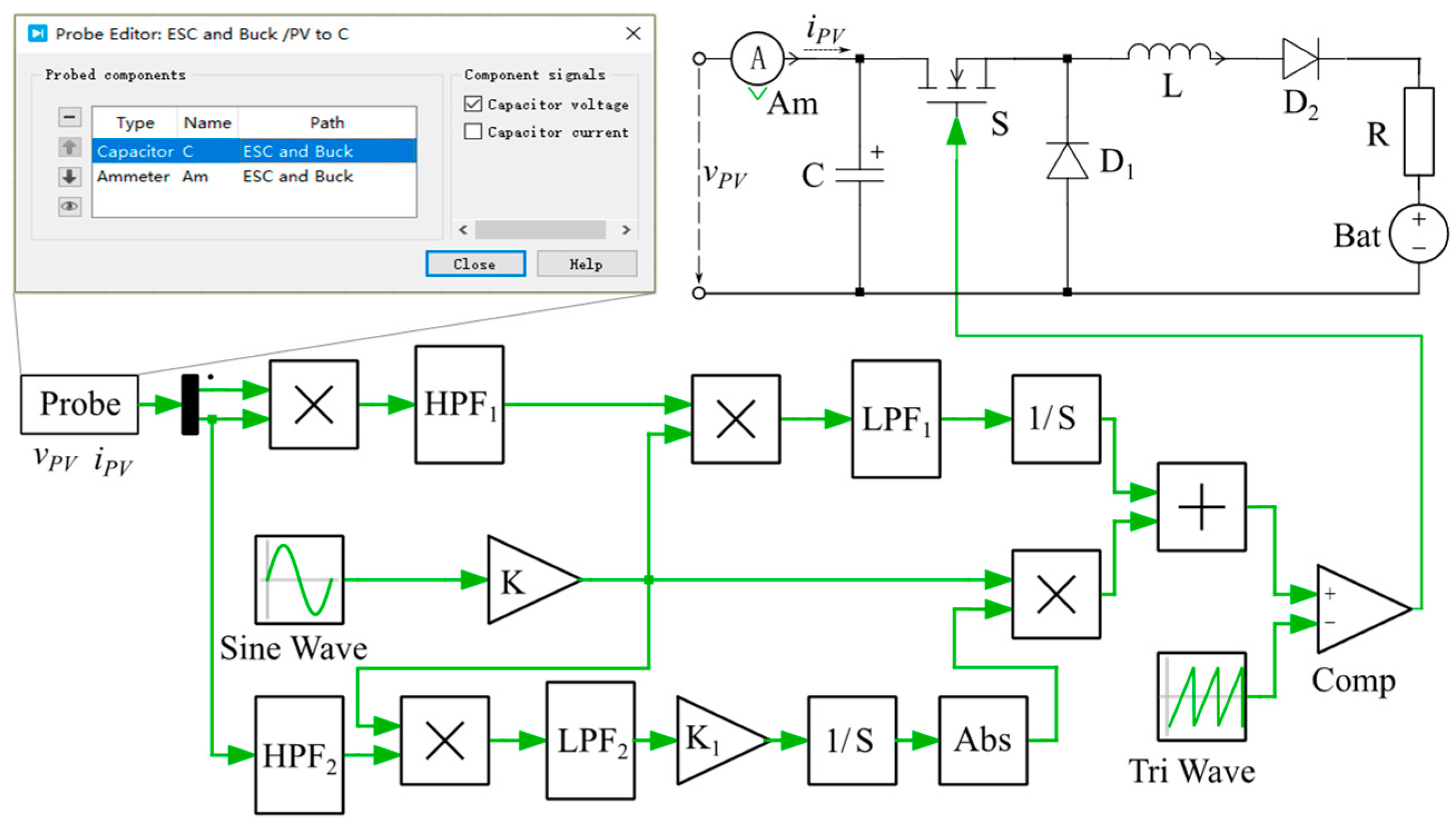
4.1. Extremum-Seeking Control
4.2. Maximum Power Converter
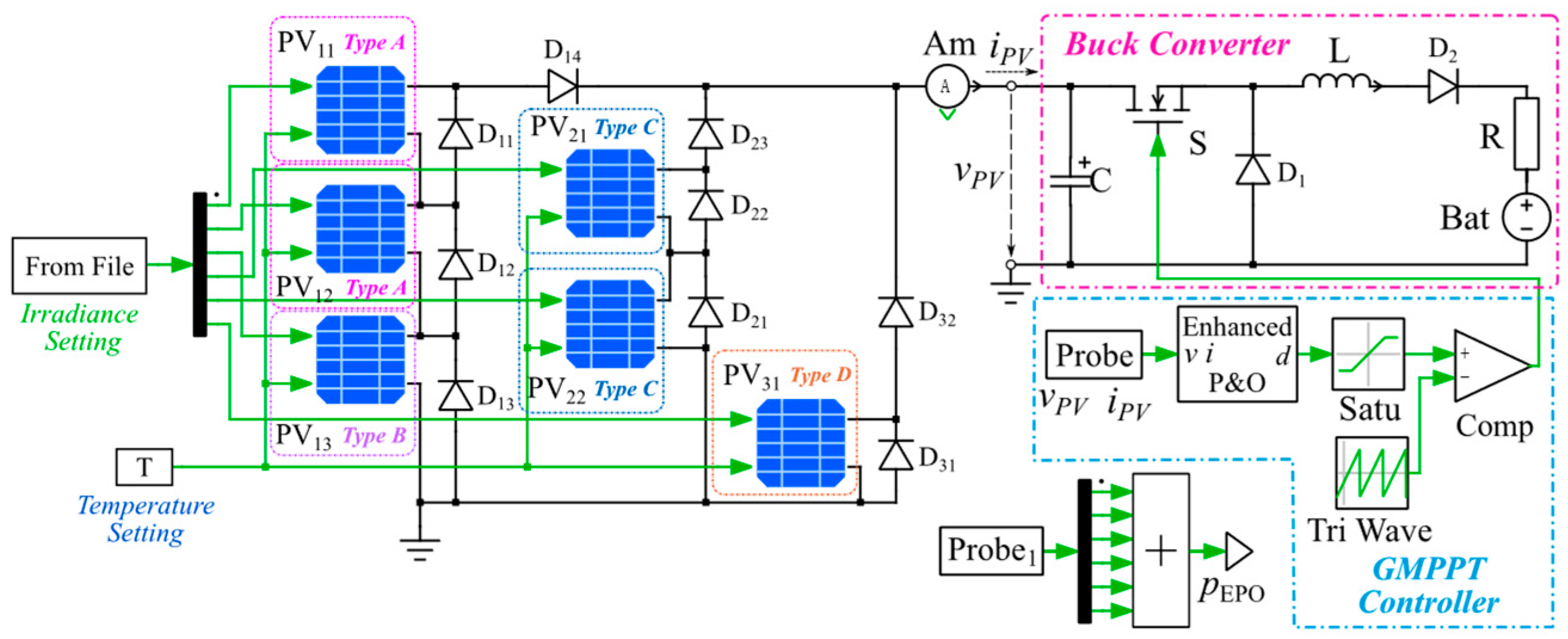
5. System Modeling and Simulation
5.1. System Modeling
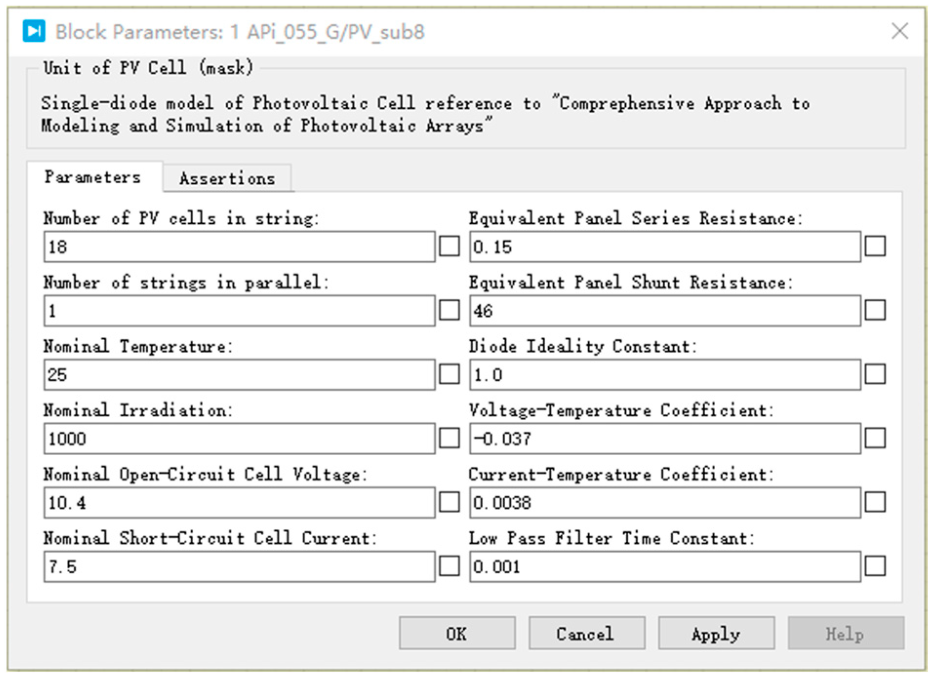
5.1.1. Modeling of PV Modules
5.1.2. Modeling of Equalization Circuit
5.1.3. Modeling of ESC Algorithms and Maximum Power Converter
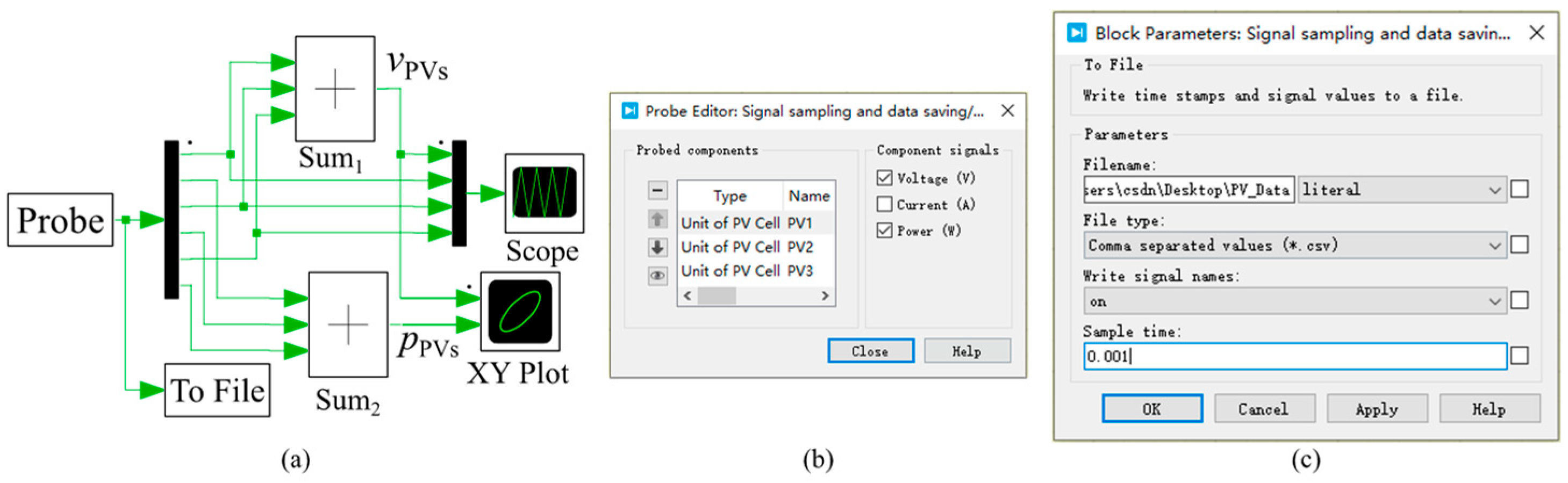
5.1.4. Modeling of Signal Sampling, Display, and Data Storage
5.2. Simulation Parameter Settings
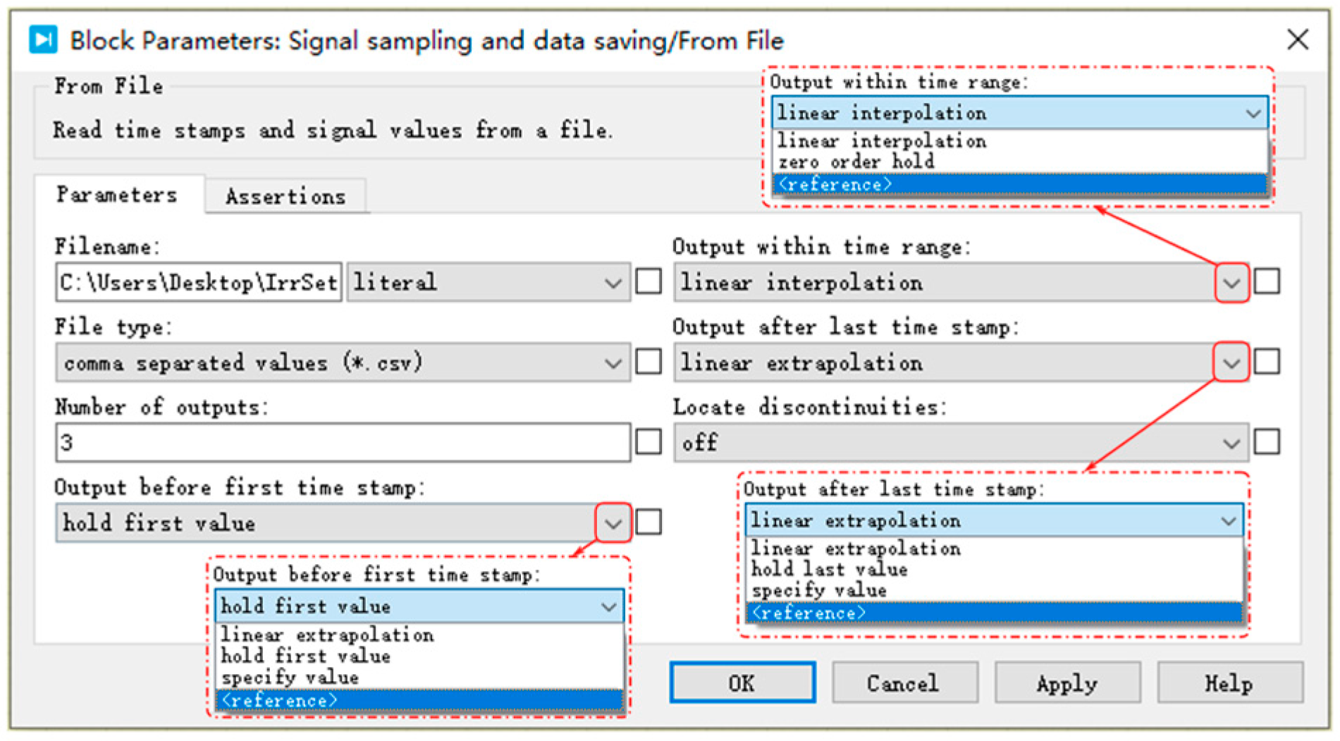
5.2.1. Irradiance Settings
5.2.2. Model Parameter Settings
5.3. Simulation of Series/Parallel-Connected PV Generation System
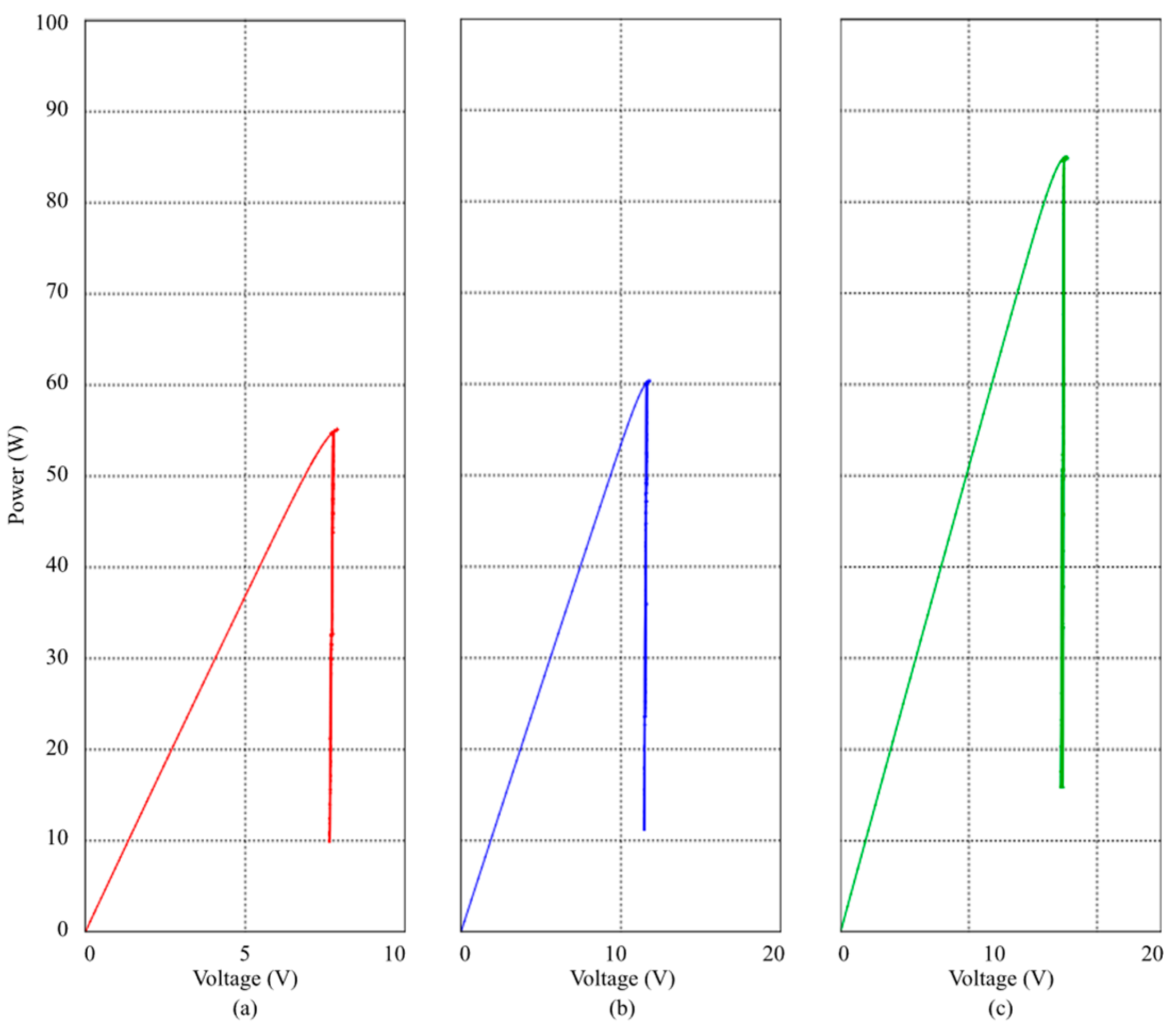
5.3.1. Simulation of Series-Connected PV Generation System
5.3.2. Simulation of Parallel-Connected PV Generation System
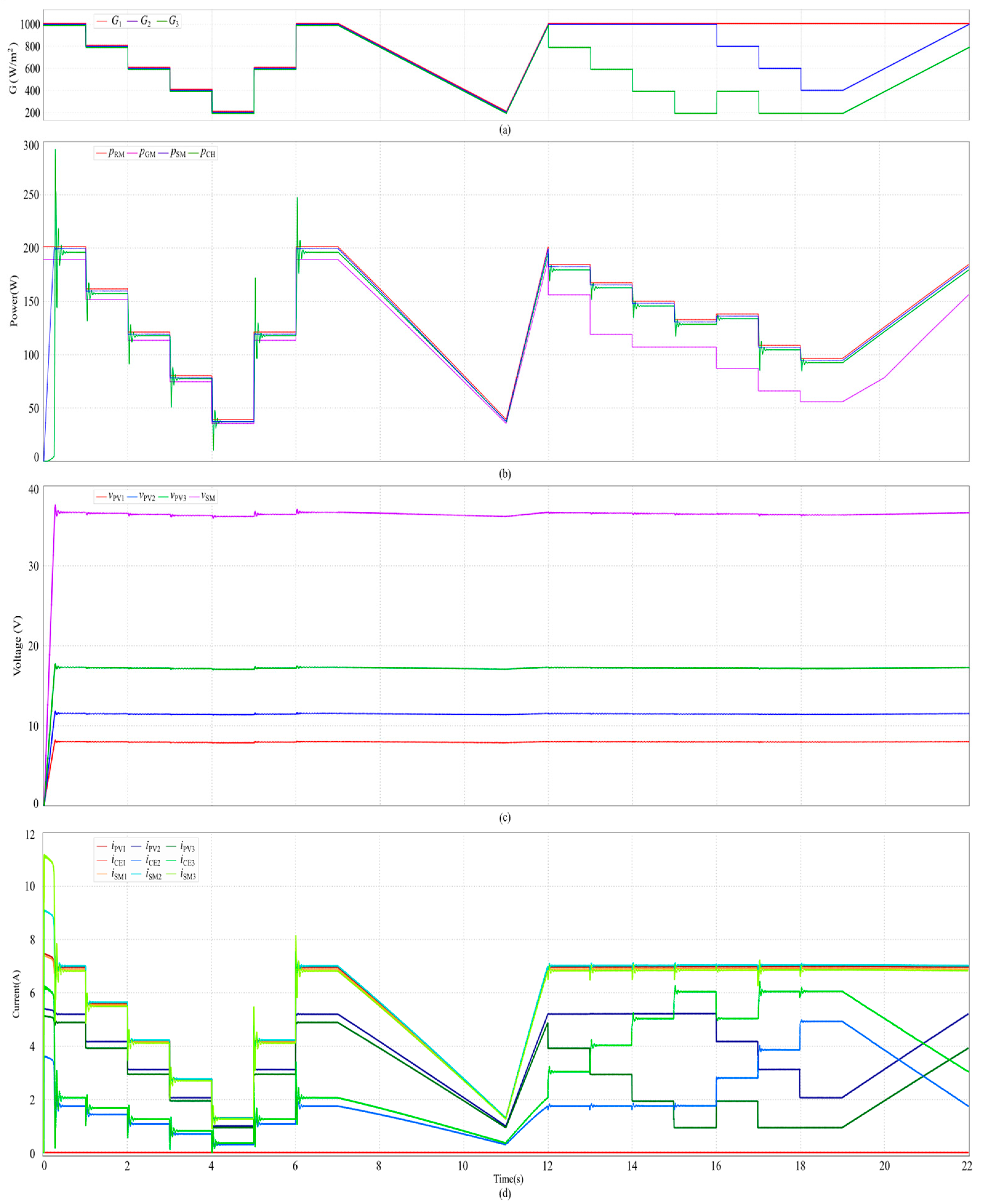
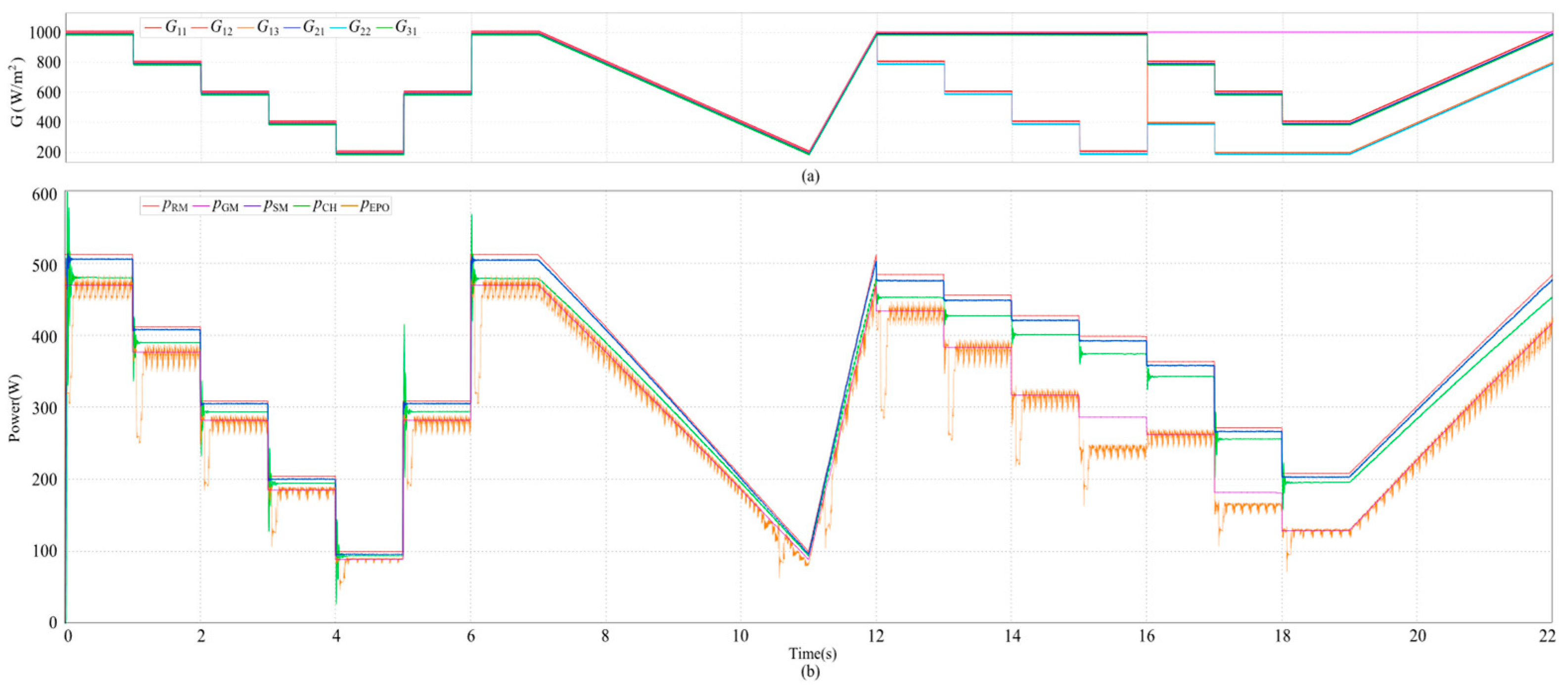
5.4. Simulation of Mixed-Connection PV Generation System
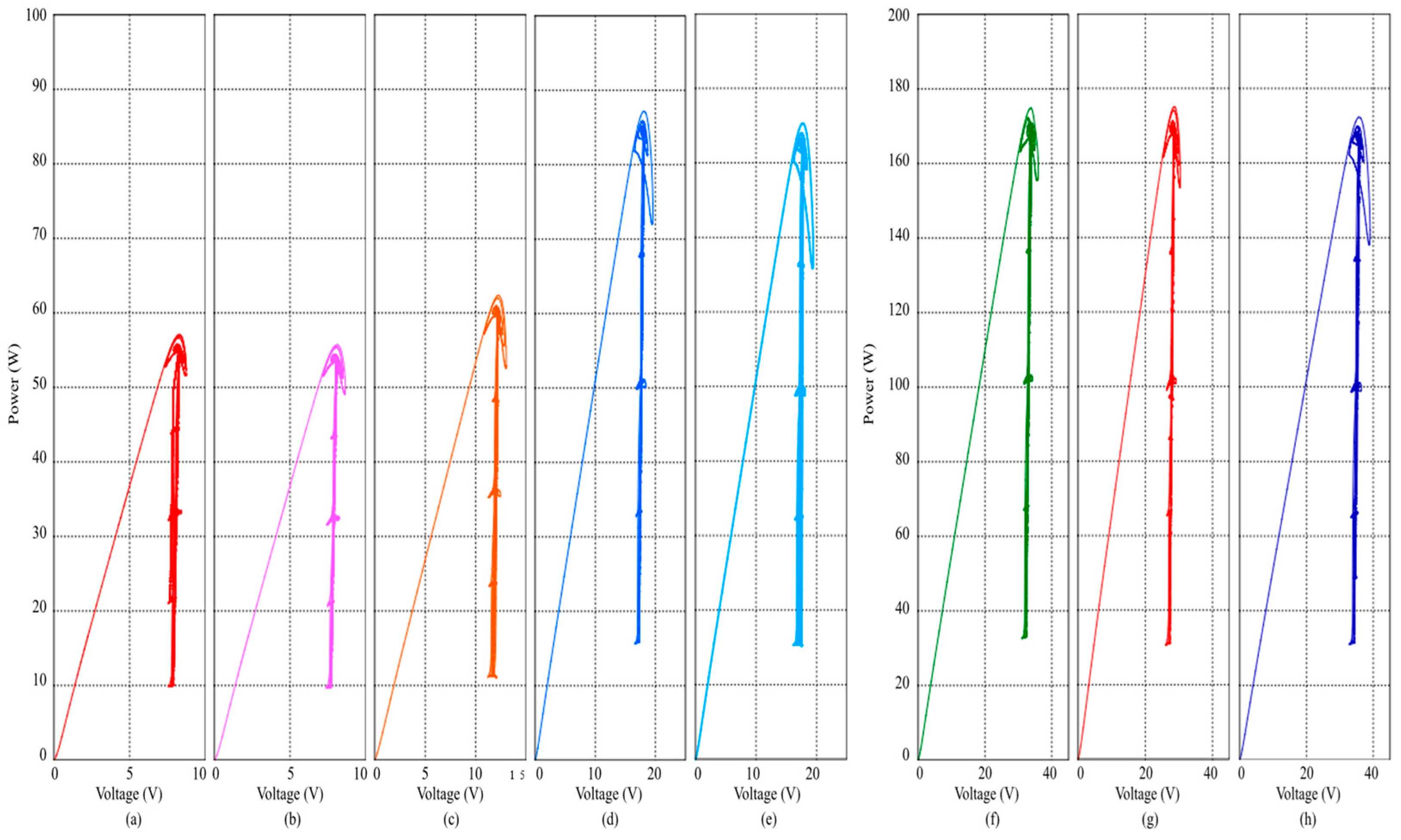
5.5. Simulation Data Processing
6. Discussion of Simulation Results
7. Conclusions
Author Contributions
Funding
Data Availability Statement
Acknowledgments
Conflicts of Interest
References
- Wang, E.; De Bono, A.; Wong, I. A Case Study: Designing a Sustainable Recreational Vehicle for the Emerging Market through Computer-Aided Design Process. Comput. Aided Des. Appl. 2014, 11, S27–S35. [Google Scholar] [CrossRef]
- Belhachat, F.; Larbes, C. Comprehensive Review on Global Maximum Power Point Tracking Techniques for PV Systems Subjected to Partial Shading Conditions. Sol. Energy 2019, 183, 476–500. [Google Scholar] [CrossRef]
- Yamaguchi, M.; Masuda, T.; Araki, K.; Sato, D.; Lee, K.; Kojima, N.; Takamoto, T.; Okumura, K.; Satou, A.; Yamada, K.; et al. Development of High-efficiency and Low-cost Solar Cells for PV-powered Vehicles Application. Prog. Photovolt. 2021, 29, 684–693. [Google Scholar] [CrossRef]
- Mohammad, A.; Zamora, R.; Lie, T.T. Integration of Electric Vehicles in the Distribution Network: A Review of PV Based Electric Vehicle Modelling. Energies 2020, 13, 4541. [Google Scholar] [CrossRef]
- Häberlin, H. Photovoltaics: System Design and Practice, 1st ed.; Wiley: Hoboken, NJ, USA, 2012; ISBN 978-1-119-99285-1. [Google Scholar]
- Chu, G.; Wen, H.; Yang, Y.; Wang, Y. Elimination of Photovoltaic Mismatching With Improved Submodule Differential Power Processing. IEEE Trans. Ind. Electron. 2020, 67, 2822–2833. [Google Scholar] [CrossRef]
- Nadeem, A.; Hussain, A. A Comprehensive Review of Global Maximum Power Point Tracking Algorithms for Photovoltaic Systems. Energy Syst. 2023, 14, 293–334. [Google Scholar] [CrossRef]
- Yuan, J.; Zhao, Z.; Liu, Y.; He, B.; Wang, L.; Xie, B.; Gao, Y. DMPPT Control of Photovoltaic Microgrid Based on Improved Sparrow Search Algorithm. IEEE Access 2021, 9, 16623–16629. [Google Scholar] [CrossRef]
- Wang, F.; Zhu, T.; Zhuo, F.; Yang, Y. Analysis and Comparison of FPP and DPP Structure Based DMPPT PV System. In Proceedings of the 2016 IEEE 8th International Power Electronics and Motion Control Conference (IPEMC-ECCE Asia), Hefei, China, 22–26 May 2016; IEEE: Piscataway, NJ, USA, 2016; pp. 207–211. [Google Scholar]
- Jeong, H.; Lee, H.; Liu, Y.-C.; Kim, K.A. Review of Differential Power Processing Converter Techniques for Photovoltaic Applications. IEEE Trans. Energy Convers. 2019, 34, 351–360. [Google Scholar] [CrossRef]
- Jeon, Y.-T.; Lee, H.; Kim, K.A.; Park, J.-H. Least Power Point Tracking Method for Photovoltaic Differential Power Processing Systems. IEEE Trans. Power Electron. 2017, 32, 1941–1951. [Google Scholar] [CrossRef]
- Shenoy, P.S.; Kim, K.A.; Krein, P.T. Comparative Analysis of Differential Power Conversion Architectures and Controls for Solar Photovoltaics. In Proceedings of the 2012 IEEE 13th Workshop on Control and Modeling for Power Electronics (COMPEL), Kyoto, Japan, 10–13 June 2012; IEEE: Piscataway, NJ, USA, 2012; pp. 1–7. [Google Scholar]
- Chu, G.; Wen, H.; Ye, Z.; Li, X. Design and Optimization of the PV-Virtual-Bus Differential Power Processing Photovoltaic Systems. In Proceedings of the 2017 IEEE 6th International Conference on Renewable Energy Research and Applications (ICRERA), San Diego, CA, USA, 5–8 November 2017; IEEE: Piscataway, NJ, USA, 2017; pp. 674–679. [Google Scholar]
- Chu, G.; Wen, H.; Jiang, L.; Hu, Y.; Li, X. Bidirectional Flyback Based Isolated-Port Submodule Differential Power Processing Optimizer for Photovoltaic Applications. Sol. Energy 2017, 158, 929–940. [Google Scholar] [CrossRef]
- Shi, F.; Song, D. A Novel High-Efficiency Double-Input Bidirectional DC/DC Converter for Battery Cell-Voltage Equalizer with Flyback Transformer. Electronics 2019, 8, 1426. [Google Scholar] [CrossRef]
- Shahid, H.; Kamran, M.; Mehmood, Z.; Saleem, M.Y.; Mudassar, M.; Haider, K. Implementation of the Novel Temperature Controller and Incremental Conductance MPPT Algorithm for Indoor Photovoltaic System. Sol. Energy 2018, 163, 235–242. [Google Scholar] [CrossRef]
- Martinez Lopez, V.; Žindžiūtė, U.; Ziar, H.; Zeman, M.; Isabella, O. Study on the Effect of Irradiance Variability on the Efficiency of the Perturb-and-Observe Maximum Power Point Tracking Algorithm. Energies 2022, 15, 7562. [Google Scholar] [CrossRef]
- Alik, R.; Jusoh, A. An Enhanced P&O Checking Algorithm MPPT for High Tracking Efficiency of Partially Shaded PV Module. Sol. Energy 2018, 163, 570–580. [Google Scholar] [CrossRef]
- Tsobze, S.K.; Njomo, A.F.T.; Naoussi, S.R.D.; Kenne, G. A New Modified ESC Algorithm for MPPT Applied to a Photovoltaic System for Power Losses Mitigation under Varying Environmental Conditions. Int. J. Dynam. Control 2023, 11, 354–369. [Google Scholar] [CrossRef]
- Tan, Y.; Nešić, D.; Mareels, I. On Non-Local Stability Properties of Extremum Seeking Control. Automatica 2006, 42, 889–903. [Google Scholar] [CrossRef]
- Ghods, N.; Krstic, M. Source Seeking with Very Slow or Drifting Sensors. J. Dyn. Syst. Meas. Control 2011, 133, 044504. [Google Scholar] [CrossRef]
- Krstic, M.; Ghaffari, A.; Seshagiri, S. Extremum Seeking for Wind and Solar Energy Applications. Mech. Eng. 2014, 136, S13–S21. [Google Scholar]
- Leyva, R.; Olalla, C.; Zazo, H.; Cabal, C.; Cid-Pastor, A.; Queinnec, I.; Alonso, C. MPPT Based on Sinusoidal Extremum-Seeking Control in PV Generation. Int. J. Photoenergy 2012, 2012, 672765. [Google Scholar] [CrossRef]
- Bizon, N. Global Maximum Power Point Tracking Based on New Extremum Seeking Control Scheme. Prog. Photovolt. Res. Appl. 2016, 24, 600–622. [Google Scholar] [CrossRef]
- Stornelli, V.; Muttillo, M.; De Rubeis; Nardi, I. A New Simplified Five-Parameter Estimation Method for Single-Diode Model of Photovoltaic Panels. Energies 2019, 12, 4271. [Google Scholar] [CrossRef]
- Kottas, T.L.; Boutalis, Y.S.; Karlis, A.D. New Maximum Power Point Tracker for PV Arrays Using Fuzzy Controller in Close Cooperation With Fuzzy Cognitive Networks. IEEE Trans. Energy Convers. 2006, 21, 793–803. [Google Scholar] [CrossRef]
- Ding, K.; Zhang, J.; Bian, X.; Xu, J. A Simplified Model for Photovoltaic Modules Based on Improved Translation Equations. Sol. Energy 2014, 101, 40–52. [Google Scholar] [CrossRef]
- Belhachat, F.; Larbes, C. Survey and Classification of Hybrid GMPPT Techniques for Photovoltaic System under Partial Shading Conditions. ENP Eng. Sci. J. 2022, 2, 31–46. [Google Scholar] [CrossRef]
- Vijayalekshmy, S.; Rama Iyer, S.; Beevi, B. Comparative Analysis on the Performance of a Short String of Series-Connected and Parallel-Connected Photovoltaic Array Under Partial Shading. J. Inst. Eng. India Ser. B 2015, 96, 217–226. [Google Scholar] [CrossRef]
- Velasco-Quesada, G.; Guinjoan-Gispert, F.; Pique-Lopez, R.; Roman-Lumbreras, M.; Conesa-Roca, A. Electrical PV Array Reconfiguration Strategy for Energy Extraction Improvement in Grid-Connected PV Systems. IEEE Trans. Ind. Electron. 2009, 56, 4319–4331. [Google Scholar] [CrossRef]
- Yilmaz, M.; Krein, P.T. Review of Battery Charger Topologies, Charging Power Levels, and Infrastructure for Plug-In Electric and Hybrid Vehicles. IEEE Trans. Power Electron. 2013, 28, 2151–2169. [Google Scholar] [CrossRef]
- Lee, J.-H.; Park, J.-H.; Jeon, J.H. Series-Connected Forward–Flyback Converter for High Step-Up Power Conversion. IEEE Trans. Power Electron. 2011, 26, 3629–3641. [Google Scholar] [CrossRef]
- Shang, Y.; Xia, B.; Zhang, C.; Cui, N.; Yang, J.; Mi, C.C. An Automatic Equalizer Based on Forward–Flyback Converter for Series-Connected Battery Strings. IEEE Trans. Ind. Electron. 2017, 64, 5380–5391. [Google Scholar] [CrossRef]
- Bizon, N.; Thounthong, P.; Raducu, M.; Constantinescu, L.M. Designing and Modelling of the Asymptotic Perturbed Extremum Seeking Control Scheme for Tracking the Global Extreme. Int. J. Hydrogen Energy 2017, 42, 17632–17644. [Google Scholar] [CrossRef]
- Luo, H.; Wen, H.; Li, X.; Jiang, L.; Hu, Y. Synchronous Buck Converter Based Low-Cost and High-Efficiency Sub-Module DMPPT PV System under Partial Shading Conditions. Energy Convers. Manag. 2016, 126, 473–487. [Google Scholar] [CrossRef]
- Liu, Z.; Ma, J.; Liu, K. Research on Control Method of Neutral Point Potential Balance of T-Type Three-Level Inverter Based on PLECS. J. Phys. Conf. Ser. 2021, 2087, 012051. [Google Scholar] [CrossRef]
- Akpolat, A.N.; Yang, Y.; Blaabjerg, F.; Dursun, E.; Kuzucuoglu, A.E. Modeling Photovoltaic String in PLECS Under Partial Shading. In Proceedings of the 2019 International Conference on Power Generation Systems and Renewable Energy Technologies (PGSRET), Istanbul, Turkey, 26–27 August 2019; IEEE: Piscataway, NJ, USA, 2019; pp. 1–6. [Google Scholar]
- Allmeling, J.; Hammer, W. PLECS User Manual. Available online: https://www.plexim.com/ (accessed on 9 September 2023).


| Type | A | B | C | D |
|---|---|---|---|---|
| Ns | 18 | 24 | 36 | 66 |
| Voc (V) | 10.4 | 14.6 | 21.90 | 41.4 |
| Isc (A) | 7.5 | 5.41 | 5.14 | 5.55 |
| Pm (W) | 55.7 | 60.6 | 85.1 | 170 |
| Vm (V) | 8.1 | 11.95 | 17.72 | 33 |
| Im (A) | 6.88 | 5.07 | 4.80 | 5.16 |
| Series Connection | Parallel Connection | |||
|---|---|---|---|---|
| Without BD | With BD | Without RD | With RD | |
| Voc (V) | 24.98 | 24.98 | 14.50 | 14.59 |
| Isc (A) | 5.44 | 7.46 | 12.85 | 12.85 |
| Pm (W) | 116.27 | 116.27 | 116.27 | 116.27 |
| PGM (W) | 107.04 | 107.41 | 100.43 | 100.43 |
| PLM (W) | --- | 55.69 | 57.51 | 60.59 |
| Three Types Connected in | Four Types Connected in | |||
|---|---|---|---|---|
| Series | Parallel | Series | Parallel | |
| Voc (V) | 46.82 | 21.89 | 88.20 | 41.37 |
| Isc (A) | 7.46 | 17.97 | 7.46 | 23.49 |
| PRM (W) | 201.4 | 201.4 | 371.4 | 371.4 |
| PGM (W) | 189.27 | 144.77 | 357.44 | 194.04 |
| PLM1 (W) | 55.69 | 122.99 | 55.69 | 192.95 |
| PLM2 (W) | 108.16 | 85.02 | 276.78 | 185.15 |
| PLM3 (W) | --- | --- | --- | 170.05 |
| Power | Irradiance (W/m2) | ||||
|---|---|---|---|---|---|
| 1000 | 800 | 600 | 400 | 200 | |
| PMA (W) | 55.70 | 44.86 | 33.67 | 22.27 | 10.81 |
| PMB (W) | 60.57 | 48.59 | 36.40 | 24.08 | 11.75 |
| PMC (W) | 85.02 | 68.25 | 51.15 | 33.84 | 16.50 |
| PMD (W) | 170.02 | 136.63 | 102.45 | 67.78 | 32.99 |
| PMA + PMB + PMC (W) | 201.29 | 161.70 | 121.22 | 80.19 | 39.06 |
| PGMS (W) | 189.27 | 151.72 | 113.39 | 74.46 | 35.33 |
| PGMP (W) | 144.76 | 116.25 | 86.99 | 57.11 | 26.95 |
| 2PMA + PMB + 2PMC + PMD (W) | 512.03 | 411.44 | 308.49 | 204.08 | 99.36 |
| PGMM (W) | 469.47 | 376.42 | 281.51 | 185.18 | 88.40 |
| Model | Type | Name | Value | Unit |
|---|---|---|---|---|
| Series/ Parallel Connection | Capacitor | C1, C2, C3 | 0.1 | F |
| Capacitor | C4, C5 | 1000 | μF | |
| Inductor | Lm1, Lm2, Lm3 | 10 | μH | |
| Inductor | Lm4 | 2.2 | mH | |
| Transformer | NW1:NW:2NW3:NW4:NW5 (Series) | 38:−38:8:12:18 | --- | |
| Transformer | NW1:NW2:NW3:NW4:NW5 (Parallel) | 8:12:18:−18:18 | --- | |
| Mixed Connection | Capacitor | C11, C12, C13 | 0.1 | F |
| Capacitor | C21, C22 | 0.066 | F | |
| Capacitor | C31 | 0.033 | F | |
| Capacitor | C14, C15 | 1000 | μF | |
| Inductor | Lm11, Lm12, Lm13, Lm21, Lm22, Lm31 | 100 | μH | |
| Inductor | Lm14 | 2.2 | mH | |
| Inductor | Lm23 | 3.3 | mH | |
| Inductor | m32 | 2.7 | mH | |
| Transformer | NW11:NW12:NW13:NW14:NW15 (Tr1) | 113:−142:32:32:49 | --- | |
| Transformer | NW21:NW22:NW23:NW24 (Tr2) | 142:−142:71:71 | --- | |
| Transformer | NW31:NW32:NW33 (Tr3) | 134:−142:134 | ||
| Buck Converter | Inductor | L | 0.2 | mH |
| Resistor | R | 0.01 | Ω | |
| Battery | VBat | 12 | V | |
| Driving Signal | f | 100 | KkHz | |
| D | 0.48 | --- | ||
| ESC Controller | HPF1, HPF2 | τ | 0.01 | s |
| LPF1, LPF2 | τ | 0.02 | s | |
| Gain | K/K1 | 50/40,000 | --- | |
| Sine Wave | a/f | 0.0005/50 | V/Hz | |
| Tri Wave | f | 50 | kHz | |
| GMPPT Controller | Satu | Upper limit/Lower limit | 0.5/0.32 | --- |
| Tri Wave | f | 50 | kHz |
| Scenarios | Change Mode | Time (s) | G1 (W/m2) | G2 (W/m2) | G3 (W/m2) | PRM (W) | PGMS (W) | PGMP (W) |
|---|---|---|---|---|---|---|---|---|
| Uniform Irradiance | Step | 0–1 | 1000 | 1000 | 1000 | 201.29 | 189.27 | 144.76 |
| 1–2 | 800 | 800 | 800 | 161.70 | 151.72 | 116.25 | ||
| 2–3 | 600 | 600 | 600 | 121.22 | 113.39 | 86.99 | ||
| 3–4 | 400 | 400 | 400 | 80.19 | 74.46 | 57.11 | ||
| 4–5 | 200 | 200 | 200 | 39.06 | 35.33 | 26.95 | ||
| 5–6 | 600 | 600 | 600 | 121.22 | 113.39 | 86.99 | ||
| 6–7 | 1000 | 1000 | 1000 | 201.29 | 189.27 | 144.76 | ||
| Linear | 8 | 800 | 800 | 800 | 161.70 | 151.72 | 116.25 | |
| 9 | 600 | 600 | 600 | 121.22 | 113.39 | 86.99 | ||
| 10 | 400 | 400 | 400 | 80.19 | 74.46 | 57.11 | ||
| 11 | 200 | 200 | 200 | 39.06 | 35.33 | 26.95 | ||
| 12 | 1000 | 1000 | 1000 | 201.29 | 189.27 | 144.76 | ||
| Non-Uniform Irradiance | Step | 12–13 | 1000 | 1000 | 800 | 184.52 | 156.14 | 135.74 |
| 13–14 | 1000 | 1000 | 600 | 167.42 | 118.92 | 126.77 | ||
| 14–15 | 1000 | 1000 | 400 | 150.11 | 107.04 | 117.84 | ||
| 15–16 | 1000 | 1000 | 200 | 132.77 | 107.04 | 109.00 | ||
| 16–17 | 1000 | 800 | 400 | 138.13 | 87.02 | 108.51 | ||
| 17–18 | 1000 | 600 | 200 | 108.60 | 65.86 | 90.54 | ||
| 18–19 | 1000 | 400 | 200 | 96.28 | 55.69 | 81.44 | ||
| Linear | 20 | 1000 | 600 | 400 | 125.94 | 78.44 | 99.28 | |
| 21 | 1000 | 800 | 600 | 155.44 | 117.90 | 117.35 | ||
| 22 | 1000 | 1000 | 800 | 184.52 | 156.14 | 135.74 |
| Scenarios | Change Mode | Time (s) | G11 (W/m2) | G12 (W/m2) | G13 (W/m2) | G21 (W/m2) | G22 (W/m2) | G31 (W/m2) | PRM (W) | PGM (W) |
|---|---|---|---|---|---|---|---|---|---|---|
| Uniform Irradiance | Step | 0–1 | 1000 | 1000 | 1000 | 1000 | 1000 | 1000 | 512.03 | 469.47 |
| 1–2 | 800 | 800 | 800 | 800 | 800 | 800 | 411.44 | 376.42 | ||
| 2–3 | 600 | 600 | 600 | 600 | 600 | 600 | 308.49 | 281.51 | ||
| 3–4 | 400 | 400 | 400 | 400 | 400 | 400 | 204.08 | 185.18 | ||
| 4–5 | 200 | 200 | 200 | 200 | 200 | 200 | 99.36 | 88.40 | ||
| 5–6 | 600 | 600 | 600 | 600 | 600 | 600 | 308.49 | 281.51 | ||
| 6–7 | 1000 | 1000 | 1000 | 1000 | 1000 | 1000 | 512.03 | 469.47 | ||
| Linear | 8 | 800 | 800 | 800 | 800 | 800 | 800 | 411.44 | 376.42 | |
| 9 | 600 | 600 | 600 | 600 | 600 | 600 | 308.49 | 281.51 | ||
| 10 | 400 | 400 | 400 | 400 | 400 | 400 | 204.08 | 185.18 | ||
| 11 | 200 | 200 | 200 | 200 | 200 | 200 | 99.36 | 88.40 | ||
| 12 | 1000 | 1000 | 1000 | 1000 | 1000 | 1000 | 512.03 | 469.47 | ||
| Non-Uniform Irradiance | Step | 12–13 | 800 | 1000 | 1000 | 1000 | 800 | 1000 | 484.42 | 433.17 |
| 13–14 | 600 | 1000 | 1000 | 1000 | 600 | 1000 | 456.13 | 383.10 | ||
| 14–15 | 400 | 1000 | 1000 | 1000 | 400 | 1000 | 427.42 | 316.84 | ||
| 15–16 | 200 | 1000 | 1000 | 1000 | 200 | 1000 | 398.62 | 286.10 | ||
| 16–17 | 800 | 1000 | 400 | 800 | 400 | 800 | 363.36 | 262.22 | ||
| 17–18 | 600 | 1000 | 200 | 600 | 200 | 600 | 271.22 | 181.29 | ||
| 18–19 | 400 | 1000 | 200 | 400 | 200 | 400 | 207.84 | 128.52 | ||
| Linear | 20 | 600 | 1000 | 400 | 600 | 400 | 600 | 300.89 | 227.02 | |
| 21 | 800 | 1000 | 600 | 800 | 600 | 800 | 392.99 | 323.20 | ||
| 22 | 1000 | 1000 | 800 | 1000 | 800 | 1000 | 483.28 | 416.39 |
| Power (W) | Efficiency (%) | |||||||
|---|---|---|---|---|---|---|---|---|
| PRM | PSM | PCH | PGM | PEPO | ηT | ηS | ηG | ηE |
| 342.74 | 339.84 | 327.11 | 289.42 | 277.65 | 99.15 | 95.44 | 84.44 | 81.01 |
Disclaimer/Publisher’s Note: The statements, opinions and data contained in all publications are solely those of the individual author(s) and contributor(s) and not of MDPI and/or the editor(s). MDPI and/or the editor(s) disclaim responsibility for any injury to people or property resulting from any ideas, methods, instructions or products referred to in the content. |
© 2024 by the authors. Licensee MDPI, Basel, Switzerland. This article is an open access article distributed under the terms and conditions of the Creative Commons Attribution (CC BY) license (https://creativecommons.org/licenses/by/4.0/).
Share and Cite
Tang, D.; Siaw, F.L.; Thio, T.H.G. Power Optimization of Multi-Type Mixed-Connection Photovoltaic Generation System for Recreational Vehicles. World Electr. Veh. J. 2024, 15, 125. https://doi.org/10.3390/wevj15040125
Tang D, Siaw FL, Thio THG. Power Optimization of Multi-Type Mixed-Connection Photovoltaic Generation System for Recreational Vehicles. World Electric Vehicle Journal. 2024; 15(4):125. https://doi.org/10.3390/wevj15040125
Chicago/Turabian StyleTang, DaiBin, Fei Lu Siaw, and Tzer Hwai Gilbert Thio. 2024. "Power Optimization of Multi-Type Mixed-Connection Photovoltaic Generation System for Recreational Vehicles" World Electric Vehicle Journal 15, no. 4: 125. https://doi.org/10.3390/wevj15040125