Article

Quantifying the State of the Art of Electric Powertrains in Battery Electric Vehicles: Comprehensive Analysis of the Tesla Model 3 on the Vehicle Level

Institute of Automotive Technology, Department of Mobility Systems Engineering, TUM School of Engineering & Design, Technical University of Munich, Boltzmannstr. 15, 85748 Garching, Germany
*
Author to whom correspondence should be addressed.
World Electr. Veh. J. 2024, 15(6), 268; https://doi.org/10.3390/wevj15060268
Submission received: 25 April 2024 / Revised: 7 June 2024 / Accepted: 14 June 2024 / Published: 18 June 2024

Abstract

:
Data on state-of-the-art battery electric vehicles are crucial to academia; however, these data are not published due to non-disclosure policies in the industry. As a result, simulation models and their analyses are based on assumptions or insider information. To fill this information gap, we present a comprehensive analysis of the electric powertrain of a Tesla Model 3 Standard Range Plus (SR+) from 2020 with lithium iron phosphate (LFP) cells, focusing on the overall range. On the vehicle level, we observe the resulting range in multiple test scenarios, tracing the energy path from source to sink by conducting different test series on the vehicle dynamometer and through alternating current (AC) and direct current (DC) charging measurements. In addition to absolute electric range tests in different operating scenarios and electric and thermal operation strategies on the vehicle level, we analyze the energy density and the power unit’s efficiency on the component level. These tests are performed through procedures on the chassis dynamometer as well as efficiency analysis and electric characterization tests in charge/discharge scenarios. This study includes over 1 GB of attached measurement data on the battery pack and vehicle level from the lab to the real-world environment available as open-source data.

1. Introduction

Driven by governments’ climate change policies, electrifying road traffic is politically motivated and subsidized. The share of electrified vehicles in the transportation sector is rising, reaching an increased registration share of 25% in 2023 compared to the same period last year [1]. In 2021, European Union (EU) member states agreed on achieving a reduction in Greenhouse gas (GHG) emissions by 90% within the terms of the European Climate Law [2]. The law restricts CO 2 emissions in urban traffic until eventually only locally zero-emission propulsion systems will be allowed. The transportation sector is a significant contributor to carbon emissions, and road transport accounts for around 72% of EU GHG emissions within the transportation sector [3]. Passenger cars contribute up to 61% of that share [3]. By 2030, the EU is planning to reduce CO 2 emissions by 55% in the passenger car sector compared to the carbon emission levels of 1990 [4].
This has encouraged manufacturers worldwide to announce ambitious plans to electrify their fleets. Manufacturers are investing greatly in the development of electric vehicles to ensure a competitive advantage, meaning that the technology of electric vehicles is improving rapidly [5]. Electric mobility is becoming more attractive due to continuously improving customer-relevant features such as vehicle range and refinement. Taking a closer look at battery technology, energy densities have massively increased in the past ten years, and are expected to increase further [6]. Simultaneously, costs for cells and battery packs are falling, which makes battery electric vehicle (BEV)models more affordable; they are expected to reach the total cost of ownership (TCO) level of internal combustion engine (ICE) powered vehicles in 2025 [7].
In addition to the automotive industry, academia has contributed to research and development (R&D) of electric vehicles. State-of-the-art knowledge and data about BEVs and their components can allow researchers to find potential strategies to optimize and develop new concepts. Unfortunately, the industry usually does not share its developments, which makes it challenging to analyze these concepts in depth [8].
Several studies have provided access to data on the components and (to a limited extent) vehicle level of BEVs. On the component level, Momen et al. [9] observed state-of-the-art of electric machines for the Chevrolet Bolt and generated an efficiency map. Unfortunately, no other powertrain components were observed. In contrast, Sarlioglu et al. [10] investigated electric machines, power electronics, and batteries of hybrid and fully electric vehicles; however neither the effects between the components nor the results on the vehicle’s overall performance were discussed.
Kovachev et al. [11] focused on investigating the powertrain on the vehicle level. They disassembled the battery pack (apparently of a first-generation Nissan Leaf ZE0) and analyzed it regarding its safety. Although their study was extensive, no performance tests on the vehicle were recorded or analyzed. Löbberding et al. [12] provided energy densities for BEVs on multiple levels; however, their data were based on several different sources, as comprehensive data were unavailable. The most extensive data collection is found in the work of Oh et al. [13]. In this study, tests on 383 vehicles were conducted; but more importantly, 27 BEVs were tested in order to quantify the state-of-the-art of their electric powertrains. Data were recorded using the onboard diagnosis (OBD)-II interface.
The advanced vehicle testing and evaluation study (AVTE), performed by the collaborative efforts of different American institutions led by the National Energy Technology Laboratory (NETL) [14], first determined vehicle performance on both the component and vehicle levels. The necessary impetus to conduct such an analysis was provided by the AVTE itself, where 30 vehicles were tested between 2011 and 2018. The results of those studies included battery pack capacity, charging efficiency, and energy consumption on the vehicle level as well as battery discharge tests and temperature analysis during battery cycling on the component level. Note that most of these vehicles are no longer state-of-the-art. This collection of current studies reinforces the statement that few facts about the current state-of-the-art of electric vehicle design and operating strategy on the system level have been disclosed.
As a reference for currently produced mass-series electric vehicles and their state of the art, especially in terms of their energy storage systems, a comprehensive analysis of our research group (EV Lab of the Institute of Automotive Technology at the Technical University of Munich) was presented by Wassiliadis et al. [15], where a Volkswagen ID.3 Performance from 2020 was tested on the vehicle, battery pack, module, and cell levels. Our group’s research focused on the customer-relevant features of range, efficiency, and lifetime, providing data from the cell level up to the vehicle level. Specifically, studies were carried out on a Tesla Model 3 at the vehicle level, focusing on specific modules such as evaluating driving assistance functions [16] and thermal management system in comparison to other Tesla models [17]. In addition, Ank et al. [18] provided a teardown analysis of Tesla’s cylindrical cells on the component level.
That previous work provides the underlying inspiration for the present study, which aims to provide further vehicle data on one of the most prominent electric vehicles on the current market. The vehicle in this study is the third most widely sold electric vehicle, excluding plug-in hybrids, with the second-most sales among electric vehicles in 2022 [19]. Thus, researchers can have reference to different electric vehicles and cell chemistry, specifically, the Volkswagen ID.3 for nickel cobalt manganese oxide Li(NixCoyMnz)O2 (NMC) cells and the Tesla Model 3 for LFP cells. To ensure as much accuracy as possible, the test procedures are performed comparably. This work only analyzes the Tesla Model 3, without comparing it to the vehicle in the previous study; however, this study does split the measurements between the vehicle and component levels. Although measurements on Tesla’s prismatic LFP cells were conducted, the investigated cells did not show reasonable internal resistance behavior during aging or electrical response to pulse testing. As the cells were of unknown mileage and history, the results led to suspicions that improper stress may have been applied to them before testing, which led to the decision to focus on the vehicle level in this study.

1.1. Contributions

This study presents a detailed examination of the electric powertrain of the Tesla Model 3 SR+ 2020 along with its LFP cells and components. Based on experiments on the vehicle level, customer-relevant properties are evaluated by analyzing efficiency and range. In addition, operation strategies are investigated, focusing on optimizing the charging duration and extending the battery’s lifetime. These investigations will ultimately lead to observations of the current state-of-the-art and disclose optimization potentials in which BEVs can be improved. With the provided results and data, researchers have the chance to compare their own research to the current state-of-the-art and parameterize their simulation models. The main contributions of this study can be summarized as follows:
  • Geometry, mass, and capacity determination for energy density calculations at multiple levels.
  • Quantification of the power unit’s efficiency in various state of charge (SOC) levels.
  • Experimental quantification of the electric range of the vehicle in official and real driving test scenarios.
  • Analysis of operation strategies on charging processes and cell balancing.
  • Open access to extensive experimental data containing 1 GB of test data on the battery and vehicle levels and over 228 individual tracks (a total distance of 6207 km).

1.2. Layout

The structure of this article is partitioned between efficiency analysis on the component level, range tests on the vehicle level, and thermal and electric strategies during operation. In Section 2, the vehicle under test is introduced along with the test procedures performed on the vehicle level. This is followed by Section 3, in which we present our analysis of the battery pack and its inner structure. Measurements are performed on both the cell and vehicle levels. From the battery, the power unit, which includes the power electronics and the electric machine, is analyzed regarding its efficiency. Efficiency maps are conducted for different software versions and different SOC levels. Subsequently, on the vehicle level, we investigate the overall range of the vehicle. The range in different driving cycles and constant speed levels is discussed and collapsed into the different energy loss shares. Subsequently, strategies for improving the operation of the vehicle in terms of charging performance and battery lifetime are investigated in real-world driving situations. Finally, we summarize these results and conclude the paper in Section 4.

2. Material and Methods

In this section, the vehicle under study is introduced and the technique of reading its internal communication is described. The test setup of the battery cells is explained, followed by the description of all experimental techniques applied in this study.

2.1. Vehicle under Test and Data Acquisition

Following its start of production in 2017, the Tesla Model 3 has been available in several different configurations. Tesla started out producing the rear-wheel drive (RWD) “Long Range” model containing a battery capacity of 79.5 kW h, which was offered until June 2019. The different RWD versions achieve 250 N m of peak torque, a 225 km/h top speed, and 0–100 km acceleration times between 5.8 s and 5.0 s. They differ mainly in their battery capacities, ranges, and fast charging capabilities [20]. Between October 2018 and March 2019, the RWD “Mid Range” version with a battery capacity of 65 kW h [21] was offered. Between March 2019 and November 2021, two RWD versions called “Standard Range” and “Standard Range Plus” were available, both containing 53.6 kW h; in the “Standard Range” version, only 50 kW h were usable [22,23]. Starting from November 2023, the currently available RWD version began to be manufactured, containing 62 kW h [24]. In addition, in 2018 Tesla started producing dual-motor all-wheel drive (AWD) versions classified as “Long Range” and “Performance” (79.5 kW h) [25,26]. The capacity varies between different versions of the Model 3, as does the cell setup. In the US market, Tesla installs cells with lithium nickel cobalt aluminium oxide (NCA) chemistry as their first option. After using Panasonic 18,650 cells for some time, they began to use larger and more energy-dense 21,700 cells. For the Chinese market, prismatic cells with LFP cell chemistry are installed in the RWD version [27]. In the European market, both cell chemistries have been sold.
The vehicle under study here is a “Standard Range Plus” model from late 2020, which uses LFP cells. The vehicle was acquired at a regular dealership to ensure test results for an unmodified mass-production vehicle. The mass of the empty vehicle was measured as 1755 kg using FLP wheel-load scales in combination with a DFW-K series terminal (DINI ARGEO S.r.l., Modena, Italy). Considering a driver’s mass of 75 kg as per the EU Regulation [28], an empty mass of 1845 kg was calculated. This is less than 1% below than the 1861 kg stated by the manufacturer in the vehicle’s Certificate of Conformity (CoC) [29]. In the CoC, the manufacturer claims an overall range of 440 km, as per the Worldwide Harmonized Light Vehicles Test Procedure (WLTP), maximum continuous power of 100 kW (for 30 min), and 239 kW of peak power with an internal permanent magnet synchronous reluctance motor (IPM-SynRM) [22]. The full vehicle specifications are included in Table A1. The measurements of the vehicle were performed on public roads, on an airfield taxiway for the coast-down test, and on a vehicle dynamometer, where an automated throttle and brake control was designed and applied to achieve reproducible results, as shown in Figure A2a.
During the measurements on the vehicle level, data were collected via the controller area network (CAN) communication of the vehicle. Through a direct connection to the wire harness of the CAN bus, data were recorded by reading the entire CAN traffic and subsequently converted into physical values by a translation file [30] containing all relevant message identifiers (IDs) as well as their respective conversion factors and offsets.

2.2. Experimental Techniques

The following subsections explain the methods and boundary conditions of all test setups and the equipment used from the cell to the vehicle level.

2.2.1. Open-Circuit Voltage Determination and Differential Capacity Analysis

Cell-level and vehicle-level pseudo-open circuit voltage (pOCV) measurements were conducted to examine the transferability of battery-specific characteristics in the differential voltage analysis (DVA) from cell to vehicle. The aim was to receive a close-to-equilibrium pOCV curve from the lower to the upper voltage boundaries by applying a low current in order to reduce the impact of over-potentials. Furthermore, by integrating the current signal, a comparison can be drawn based on the extractable capacity during a complete charging cycle.
The vehicle-level pOCV from the vehicle under study was discharged by driving to an SOC indication of 0% in the user interface (UI) followed by running the cabin heater until the vehicle systems shut down automatically. After a rest period for balancing, the vehicle was recharged at an ambient temperature of 20 °C and the lowest selectable power setting on the onboard AC charging system. Indicated as “4 A”, we measured about 920 W of power at 230 V effective mains voltage charge input. Therefore, the actual DC side charge current continuously decreases with rising pack voltage. However, it is sufficiently constant at around 3 A ( ± 20 % to be modeled as a C / 57 constant current (CC) charge process. The voltages of the pack and all individual cells were recorded using the battery management system (BMS) output on the vehicle’s CAN communication during the procedure, enabling evaluation of cell scattering within the pack. Furthermore, the procedure was carried out twice, one time at an odometer reading of 390 km and 17 months later at 25,716 km, enabling the comparison of two different aging states.
For the cell measurements, we disassembled the 25 hardcase cells from the additionally acquired teardown battery module (Appendix C) by removing the beams, end caps, cooling plate, and bus bars to enable single-cell tests. Separating the single cells from the module housing leads to loss of both the module-induced stiffness and the initial module compression force. No external compression pressure was applied to the hard case cells during the single-cell measurements.
The cell-level measurements were conducted in a VC 3 4100 thermal camber (Vötsch GmbH, Balingen, Germany) to set the given temperature for characterization and cycling. The cell was connected to two parallel-connected channels of an MRS 6 V battery cycler (BaSyTec GmbH, Asselfingen, Germany). Each channel had a maximum current of ±300 A with a current and voltage accuracy of ±300 mA and ±1 mV, respectively. To enable friction-locked electric contact between the cells and the test system, the DC busbars were carefully bent upwards and drilled through, as shown in Figure A2f. In this way, the source and sense cables were bolted to the cell. Two Pt100 thermistors were mounted on top of the cell in order to observe the cell temperature during the measurements for safe testing.
A current of C / 57 (ca. 2.8 A, for comparability to vehicle level tests) was applied between voltage limits of 2.5 V to 3.65 V and at an ambient temperature of 20 °C to perform the pOCV measurement.
The voltage signal of the pOCV was derived using the charge results in the so-called DVA, which is an essential tool for in situ chemistry and aging characterization on the cell and electrode level [31]. Peaks in the DVA are indicators of phase transitions inside the cell, and shift/thin out over the course of aging; for this reason, they are often employed when estimating the state of health (SOH) [32,33,34].
Using Equation (1), the normalized differential voltage U D V A was calculated for every timestep in the pOCV data, wherein Q 0 is the single cell reference charge capacity. Positive values were used for both current directions to enhance comparability. An unweighted moving mean algorithm was applied to the voltage and current measurement data to reduce noise in the differentiation step. Afterwards, another application of the moving mean was carried out to make the data readable, especially in the lower-value regions.
U DVA = Q 0 d U d Q = Q 0 d U d t d t d Q = Q 0 d U I d t Q 0 Δ U I Δ t

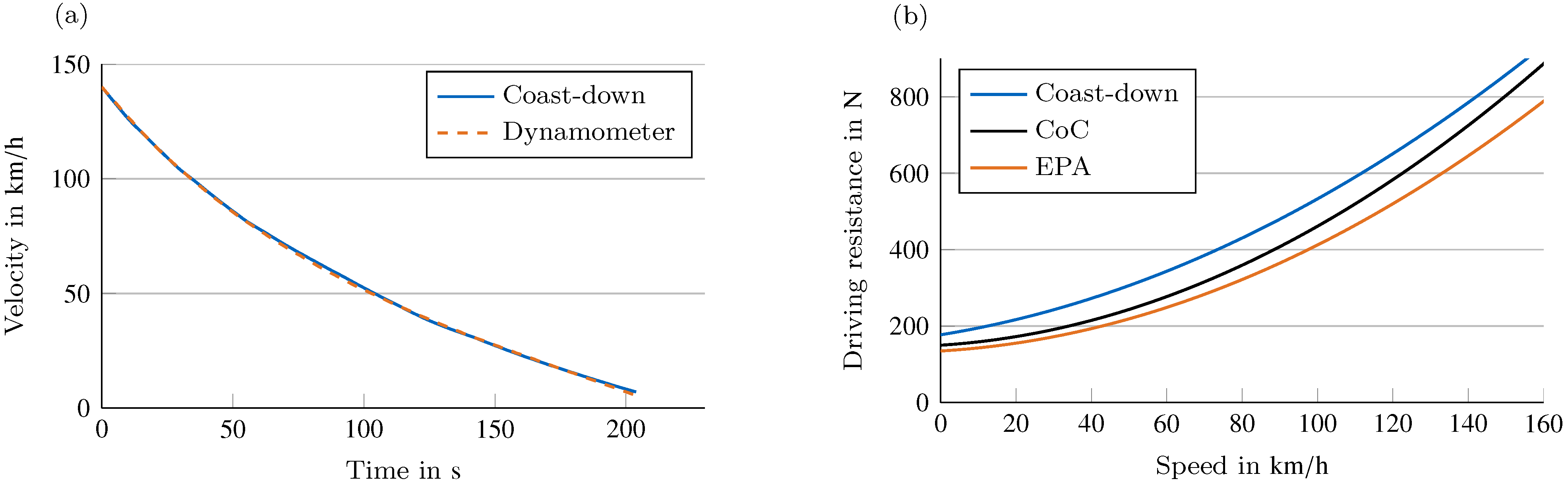
2.2.2. Vehicle Coast-Down Procedure and Driving Resistance Determination

Coast-down test procedures are generally performed to quantify the vehicle’s drag components, which is necessary in order to mirror these characteristics on a dynamometer and reach an accurate simulation of reality. The measurements were performed on a paved runway with a 1.5 km long flat and straight track, offering optimal test conditions [35]. As recommended [36], wind velocity at 2 m/s was below the threshold value of 5 m/s. The vehicle was switched into neutral gear to perform these tests; thus, neither positive nor negative torque impact is observed within the data. Additionally, measurements were taken in both directions to avoid deviations due to minor elevation differences and repeated for a total of six times each to minimize the influence of inhomogeneous surfacing and other external influences. The velocity range covered was from 140 km/h down to 15 km/h, as recommended by Liebl et al. [36]. Considering the available track length, the velocity range was split into four intervals: 120–140 km/h, 100–120 km/h, 60–100 km/h, and 15–60 km/h. After the vehicle was weighed, the components were warmed to common operating conditions by dynamic driving for 20 min. The recorded velocity profile was then used to fit the driving resistance equation:
F = m g f RR Rolling resistance + 0.5 ρ v 2 c d A Aerodynamic resistance + ( m + λ ) a Inertia
where m is the vehicle’s test mass, g is the gravitational acceleration, f RR is the rolling resistance coefficient, ρ is the air density, v is the velocity, c d is the aerodynamic drag coefficient, A is the reference frontal area, and λ is the mass equivalent inertia. In Equation (3), the rolling resistance is accounted for in the constant and the velocity-proportional term. In contrast, the inertia-related resistance is only related to the velocity-proportional term, and the quadratic term represents the aerodynamic resistance. Polynomial regression to the base function
F fit = a 0 + a 1 v + a 2 v 2 ,
yields a 0 = 177.2 N, a 1 = 5.743 N/(m/s), and a 2 = 0.2538 N/(m/s)2 as the most accurate parameters, with a root mean squared error (RMSE) of 0.67 N. A more detailed description of the procedure and its results is shown in Appendix B.

2.2.3. Vehicle Dynamometer and Charging Tests

The coast-down results were transferred to the vehicle dynamometer, a single-axis chassis dynamometer with a maximum velocity of 250 km/h (Renk GmbH, Augsburg, Germany). Three test series were performed. Within the first test series, the range of the vehicle was examined by applying internationally standardized test procedures and real-world driving scenarios. The real-world scenarios were represented by an urban track of 8.1 km, an interurban course of 20.1 km, and a highway drive of 35.2 km. The speed profiles of these public road driving situations were recorded and reproduced on the chassis dynamometer using an automated throttle and brake control. As derived from the official test procedure conditions, the total electric range in every scenario was defined as the point when the vehicle could no longer follow the target velocity. According to the international test procedures in [37], the cabin heating, ventilation, and air conditioning (HVAC) were deactivated. Figure 1 shows the velocity profiles of the real-world driving scenarios, recorded at an ambient temperature of around 23 °C and a starting SOC of around 80%.
In addition, the battery currents and voltages were recorded in order to transfer load profiles to the cell level. The relative frequency of current rates for every real-world drive cycle is shown. Because the urban drive cycle is less dynamic, the average discharging C-rate is only 0.04 C and the maximum discharging C-rate is 0.7 C , compared to the significantly more dynamic highway drive cycle reaching discharging C-rates of 0.3 C on average and 2.1 C as a maximum. According to E n e t = E d r i v e E r e c u p e r a t i o n , the net energy taken from the battery during one urban cycle is 1.3 kW h. In contrast, the net energy of one highway cycle is 7.9 kW h. This lower net energy in the urban cycle is achieved through a recuperation of 31.2%, while the highway cycle only regenerates 14.5% of its energy consumption due to less regenerative braking.
In the second test series, the electric range when driving at a constant velocity was determined, allowing the impact of individual drag components to be examined. At lower velocities, the impact of the rolling resistance dominates, while at higher velocities, aerodynamic drag is more influential. As in the first test series, automated throttle and brake control were applied. In contrast to the first test, the range was calculated using the measured energy consumption and battery capacity. For eleven velocity levels of 15 , 30 , 40 , 50 , 65 , 80 , 100 , 120 , 130 , 150 , and 160 km/h, each level was recorded at ambient temperatures of 15 °C and 30 °C to investigate the impact of the powertrain components’ temperatures and their cooling on the energy consumption. The vehicle dynamometer was in a closed chamber linked to the institute’s climate control. In combination with the outside temperature and heaters within the chamber, multiple temperature levels were reached and maintained. In addition, these tests were performed at both a low SOC level of <30% and a high SOC level of >60% in order to observe the possible influence of different DC link voltages.
The third test series focused on the efficiency of the powertrain components, especially the electric machine and inverter. After the chassis dynamometer was switched to speed control, allows the vehicle to be held at a steady state, specific load points (vehicle speed and motor torque) were measured. These load points were recorded for 20 s after the vehicle was no longer accelerating, and the respective vehicle speeds were maintained with a constant applied torque to ensure constant values during recording. Starting from a vehicle speed of 4 km/h and a motor torque of 16 N m, the torque was increased until the maximum at the respective vehicle speed was reached. This procedure was repeated at every speed level. The measurements were performed at an ambient temperature of 23 °C. The DC link (i.e., battery) voltage was kept at as constant a level as possible in order to keep the operating point of the inverter constant. The experimental setup did not allow for maintenance of an exact SOC level, as the vehicle cannot be charged while operating; therefore, all measurements were conducted in the SOC range from 30–60%, as the LFP battery chemistry shows a nearly constant voltage within that regime. It should be mentioned that the efficiency map may contain some inaccuracies compared to measurements on a motor test bench, as the temperature of the dynamometer increases slightly. In addition, the influence of the vehicle’s software version is essential, as it influences the vehicle’s torque characteristics in the so-called dyno mode, which needs to be activated on the chassis dynamometer to avoid control interventions because the front wheels are not in motion. Note that the accuracy of onboard vehicle measurements needs to be considered as well, e.g., the torque provided by the electric machine is probably not directly measured and is instead calculated within the control unit by applying signals from other sensors.
In addition to the chassis dynamometer test, charging tests were performed on the vehicle level. AC charging was performed in the UI–SOC range of 0– 100 % . To measure customer-relevant charging situations, an 11 kW wallbox charging was recorded. As shown in Figure 1, we observed a constant power (CP) charging protocol. It should be noted that the UI–SOC holds a capacity reserve, which means that the actual SOC of the cell, and consequently the pack, is higher.
To comply with the manufacturer’s charging recommendations for DC charging, the charging measurements were recorded between 10% and 80% UI–SOC. Figure 1 shows two different graphs for the DC charging process, with the blue graph describing a charging process after thermal relaxation overnight. The starting battery temperature was measured at 17.5 °C. On the other hand, for the red graph charging was started immediately after discharging the vehicle on the highway, and the battery starting temperature was recorded at 31 °C. In the operating process, the graph starts at the maximum allowed power until it is subsequently reduced. In the cold operating condition, a nearly constant voltage (CV) charging protocol was observed. Note that the charging process was not stopped manually other than the user-presetable limit SOC, which might have affected the behavior when close to reaching the preset SOC.

3. Results and Discussion

Having described the vehicle under study and all experimental techniques, we next present the results of our analysis. Starting from the components within the vehicle (i.e., the battery pack and electric power unit), we investigate the vehicle’s overall behavior by analyzing its range and thermal and electric operation strategies.

3.1. Energy Storage Analysis

This section analyses the engineering of the battery pack and its inner structures. Starting at the cell level, we then move on to consider the module and battery pack levels. In addition, the evolution of the gravimetric and volumetric energy densities is determined, and measurements taken on the cell level are compared against the results of equivalent tests on the vehicle level.

3.1.1. Energy Densities

Each battery cell disassembled in Appendix C and shown in Figure 2a displaces 1.45 dm3 and has a mass of 3.10 kg as measured on a DE 60K20N scale (KERN & SOHN GmbH, Puchheim, Germany). The measured charge capacity and energy at a low current of C / 57 are 164.4 A h and 544.7 W h, respectively. The corresponding discharge values are 166.6 A h and 542.9 W h, leading to a Coulombic efficiency of 101.3% and an energy efficiency of 99.7%. Such unusually high values could be obtained in multiple repeated tests, but did not occur at higher currents of C / 40 and C / 10 . This behavior might be caused by an accumulating offset in current measurement and/or anode overhang effects [38], which are indistinguishable from our data. For comparability to the vehicle level, the charge direction values were taken as reference for energy density calculations, which result in 176 W h kg−1 and 376 W h dm−3, respectively.
Scaled up from the cell level reference capacity, the investigated 25-cell module contains 13.6 kW h (15.3 kW h for the larger 28-cell variant). Even though only the smaller module type is considered, only minor deviations are expected for the larger one. With the overall dimensions shown in Figure 2b, the former’s total displacement was 38.4 dm3 and its mass was 84.1 kg. This results in gravimetric and volumetric energy densities of 162 W h kg−1 and 355 W h dm−3, respectively. The module’s maximum voltage is above the IEC60449 extra-low voltage threshold of 60 V, requiring additional training and safety precautions in handling and manufacturing.
Figure 3 displays the losses in gravimetric and volumetric energy densities from the cell via the module to the pack level, with 8% of the total mass and 6% of the total volume in the battery module being non-cell material (e.g., housing, cell connections, cabling, sensors, spacers, and battery electrical and thermal management).
On the battery pack level, the four modules are electrically connected in series. This leads to a theoretical electrical capacity of 164.4 A h and a total energy content of 57.7 kW h (at a nominal voltage of 351 V) when scaled up from the cell level reference values. However, as Figure 4 indicates, less charge (161.6 A h) and energy (57.0 kW h) were transferred to the vehicle level charge procedure, indicating the extent of limitations set by the manufacturer through software protecting the pack from extreme SOC ranges. Unfortunately, as the aging states differ between the two measurements on cell and vehicle level and this effect superposes the voltage limits, exact buffers cannot be quantified here.
As visible in Figure 2c, the battery pack’s height varies between the main energy storage section at 110 mm and the “penthouse” section under the rear bench seat at 315 mm. CAD modeling reveals a displaced volume of 277.4 L. At the same time, the total mass was weighed as 458 kg, including a small remainder of the coolant present after draining by opening all hose connectors and holding them below the vehicle floor level while still mounted in the vehicle. Combined with the scaled-up energy content, this leads to pack-level gravimetric and volumetric energy densities of 126 W h kg−1 and 208 W h L−1, while the values in reference to the measured pack energy are slightly lower at 125 W h kg−1 and 206 W h L−1, respectively. The module-to-pack integration losses, equaling the non-module components’ share (e.g., casing, electrical connections, battery thermal management system (BTMS), BMS, onboard charger, and DC-DC converter), consequently lie at 12% in mass and 41% in volume.

3.1.2. Comparison of the Cell and Pack pOCV and DVA

Figure 4a illustrates the pOCV versus charge throughput resulting from the procedure described in Section 2.2.1 for the cell level in terms of the charge and discharge direction between the lower and upper voltage limits stated in the manufacturer’s datasheet. Additionally, the vehicle-level charging tests in two different aging states are added to the figure, shifted by 5 A h to the right in order to best coincide with the cell-level features (specifically, the steep gradient at low SOC) as well as to compensate for the aforementioned SOC limitations at the vehicle level. As the sum of all cell voltages did not match the pack voltage, instead having an offset of ca. 5 V, the cell voltage values were corrected evenly for plotting in order to avoid accumulating tolerance errors when correcting the pack-level voltage. Examining the open circuit voltage (OCV) in Figure 4a, distinct differences are visible towards the end of charge. While both the single cell and aged vehicle experienced a characteristic steep increase in pack (and mean cell) voltage towards the charge cutoff, the new pack seems to be limited by only a few cells deviating toward high voltage and 100% SOC. The mean stays low, indicating higher potential capacity with tighter matching of cells. In fact, cell IDs 39 and 40 (as per the CAN data naming scheme, which is not traceable to physical positions) are the only two responsible for the deviation. No common identifiable vehicle charge cutoff criterion could be found in the data. The total capacity loss over a driving distance of roughly 25,000 km and nearly 1.5 years is measured to be 3.4%, which is significant albeit the short usage period.
Looking at the cell-level DVA shown in Figure 4b, the typical flat OCV profile of LFP cathodes manifests itself in generally low values, indicating no characteristic cathode-side stage transitions, as is expected on LFP cells [39,40]. In contrast, the graphite anode shows the characteristic peaks (at 23 A h, 38 A h, 45 A h, and 101 A h), indicating the (dis)appearance of lithium intercalation stages [41,42]. Here, the maxima indicate the existence of only one stage, while the minima represent the coexistence of two phases [43,44]. Depending on the relative position in the spectrum, they can serve as trend indicators for electrode storage capacities. As such, they can be used to evaluate various aging modes [45], especially in comparison to pack-level measurements (see Section 3.1.1).
Figure 4b also shows the corresponding DVA on the vehicle level for both aging states, in which a reducing capacity between the central graphite peak around 101 A h and 100% SOC can be observed with aging. This is an indicator of shifts in electrode balancing [46]. Due to the fact that the peak heights of other relative capacities remain primarily constant, any change in anode properties is deemed to be negligible. Thus, the shift in electrode balancing is attributed to the degradation mode loss of lithium inventory (LLI) due to lithium-consuming side reactions (e.g., electrode interface growth) [32,40,47,48]. In a general comparison between the cell-level and two vehicle-level measurements, the investigated cell seems to be in an aging state that falls between the aging state of the new and aged vehicle. The battery pack with 106 cells in series makes it possible to determine each cell’s current using a single pack-level current sensor. Additionally, the voltage across each cell is measured for BMS functionalities. Therefore, it is possible to precisely determine the DVA for each cell. The left close-up plot in Figure 4b focuses on the characteristic graphite peak in LFP cells for the new vehicle state. It is visible that the y-position of the peaks only varies slightly, forming a broad plateau. However, there is a significant distribution of the peaks among the X-axis of about 7 A h, scattering around the peak of the pack level DVA. This distribution is likely due to cell-to-cell variations in the capacities and internal resistances from production tolerance and the initial formation process. Additionally, it is also unknown if the cells are matched prior to the battery pack assembly. It is assumed that close matching of cells would reduce the width of the distribution of the cell-level DVAs in relation to the pack-level DVA.
The close-up plot on the right-hand side in Figure 4b depicts the cell level DVAs for the aged vehicle state. It visually appears as if a notable number of cells are shifted to the left, indicating significant advancement of degradation. Profound knowledge and degradation maps are necessary for the exact determination of the degradation modes at hand, which can be time-consuming and challenging even at the cell level in laboratory conditions [49]. However, the DVA curves of single cells inside a battery pack can be used for peak tracking over time, especially as the sample frequency and resolution of the extracted CAN measurements seem to provide sufficient data quality. The feasibility of such an approach has been demonstrated in [50,51,52]. Nonetheless, further research needs to be conducted on the development of DVA as an in operando diagnosis tool for battery packs during standardized charging cycles. This can enable reliable SOH estimation techniques to ensure safe operation, longevity, and reliability of the battery packs, as well as the detection and possibly the localization of single cells that are close to failure.

3.2. Power Unit Efficiency

With more efficient components in the electric powertrain, the vehicle greatly benefits in several different design aspects: first, battery size can be decreased while still reaching the same range, and thermal management can be designed more appropriately; second, there is potential for cost reduction if the components are designed correctly; third, secondary weight effects can allow the vehicle to be made lighter, resulting in higher electric ranges and better driving dynamics [53]. The investigated vehicle’s motor controller and electric machine are combined in a single power unit. In this section, its efficiency is assessed based on dynamometer measurements, as described in Section 2.2.3.

3.2.1. Efficiency Map of the Power Unit

The efficiency of the power unit, including the power electronics and electric machine, is calculated using Equation (4)
η = P mot P inv = T mot · ω mot ( U bat · I bat ) P aux
with the given mechanical power P mot provided by the motor output torque T mot and its angular velocity ω mot . The inverter’s input power P inv is given by the battery power P bat provided by its voltage U bat and current I bat minus the power for the auxiliary components P aux . Figure 5a describes the efficiency map of the investigated vehicle running software version 2021.4.18, whereas Figure 5b shows the newer version 2022.20.8. Note that both efficiency maps were conducted in the SOC range between 30–60% and with the same parameter setup on the chassis dynamometer.
In software version 2022.20.8, the highest achieved torque was reached at 320.8 N m, significantly lower than the maximum torque of 420 N m provided by [54]. However, the full torque is reachable while driving with dyno mode deactivated. According to [55], several incidents made the manufacturer reduce the maximum torque in dyno mode, as this had been used to deactivate safety functions. Comparing the maximum torque of the two efficiency maps shown here, in the older version a maximum torque of 420.0 N m is reached, which is 30.9% higher than in the newer version and meets the data stated in the CoC.
In addition to the value of the maximum torque, the behavior of the maximum torque over the motor speed is different; whereas previously there was a step implemented in the former version, only allowing for a maximum of around 200 N m until reaching a motor speed of at least 1000 1/min, the newer version allows the aforementioned reduced potential almost from the very beginning. Similar to a standard efficiency map of an electric machine [56], the older version reaches a level of constant torque during lower speed levels. In contrast, the newer version continuously decreases the maximum torque.
Investigating the areas of optimum efficiency, we do not observe the expected characteristics of a permanent magnet synchronous motor (PSM) [56,57]. The maximum efficiency of 97% in both maps is reached at low torque (either <50 N m in (a) or <70 N m in (b)) and high speed (12,000–16,000 1/min), although the optimal point of a standard PSM is expected to be at medium-to-high torque at medium speeds [56,57]. In the newer version, the area with an efficiency greater than 96% is extended into medium speeds for nearly every torque level, resulting in a more efficient version.

3.2.2. Efficiency Dependencies over SOC

Further investigations were carried out to determine the influence of the SOC on the powertrain efficiency as defined in Equation (4). For this purpose, efficiency maps were created in SOC ranges of 0–29%, 30–60% (reference), and 61–100%. Figure 6a shows the absolute efficiency differences between the low and middle SOC ranges. The maximum deviation of −3.2% can be seen at a motor speed of 876 1/min and a motor torque of 14 N m. Further distinct deviations of −1.9% and −1.1% are determined at higher motor speeds.
Figure 6b shows the absolute difference of the inverter-motor efficiency map in a range of 61–100% SOC compared to the reference efficiency map in the range of 30–60%. The maximum deviation of 1.6% can be seen at a motor speed of 1789 1/min and a motor torque of 277 N m and 16 N m. For motor speeds >10,000 1/min and motor torques >32 N m there are hardly any deviations.
The following limitations should be mentioned. First, it was determined that the maximum torque according to the vehicle’s technical specifications (in dyno mode) was not reached when running on the updated software version. Note that there was no limitation of torque when operating the vehicle at low SOC levels in either SW version. Although a defined accelerator pedal position was set, it was not possible to reproduce exact operation points. The vehicle’s speed was recorded from the dynamometer data, which varied in a small range. Although the measurement strategy ensured consistent component temperatures by alternating the recording of more and less demanding operating points, minor deviations between component temperatures were accepted. Concluding these results, it seems that the SOC level has minimal to no influence on the efficiency of the powertrain unit when considering the minor deviations in both directions (possible measurement inaccuracies) compared to the reference measurement, and especially considering the near-constant voltage range of LFP cells.

3.3. Range

By collocating the results on the battery system and the power unit, this section aims to investigate the arguably most customer-relevant feature, namely, the real-world driving range of the vehicle under study. In addition to the overall electric range of real-world driving scenarios, we present and discuss the vehicle’s range of constant speed levels at different boundary conditions. Subsequently, we determine the energy loss shares for the discussed cycles.

3.3.1. Real-World Range and Influencing Factors

Figure 7a shows the vehicle’s electric range in the internationally standardized and real-world driving cycles performed on the chassis dynamometer as described in Section 2.2.3. All range tests were performed with software version 2021.4.18. The measured WLTP range on the dynamometer was 430 km, which is only 2% smaller than the manufacturer states in the CoC.
Compared to the WLTP, the urban cycle increases the total range by 27% due to lower vehicle speed levels, and consequently lower energy consumption; moreover, regenerative braking is especially beneficial, as deceleration in the investigated urban drive cycle is comparably low and most braking events stay within the capabilities of regenerative braking, resulting in energy being fed back into the battery. In addition, fairly little mechanical braking is applied, which accounts for less wear and tear of the mechanical parts, leading to a high ratio of regained to dissipated braking energy. In a further test series, we investigated the maximum power of regenerative braking that could be achieved. Within a vehicle velocity interval from 130 km/h to 100 km/h, a maximum electrical power of 66.9 kW into the battery was reached independently from the brake pedal position and driving mode. The driving mode only impacts velocities up to 20 km/h. Including the ambient temperature, it is observed that lower temperatures result in lower ranges. Especially during regenerative braking, the regained energy level is significantly lower due to the restriction of electric braking potential at cold component temperatures. Higher temperatures also result in less tire friction and less battery internal resistance. The interurban cycle achieves a yet higher range compared to the WLTP, by 8%; due to higher vehicle velocities in the highway scenario and fewer regeneration phases, the highway scenario only reaches an electric range of 280 km, about 35% lower than the WLTP.
The additional graphs in Figure 7 compare the energy consumption (b) and its range (c) at different constant speed levels. In this test series, the ambient temperature was varied in both cases, whereas the SOC level is also varied in Figure 7c. The general observation of the four different test scenarios indicated that high ranges are achieved at an ambient temperature of 30 °C. As shown in Figure 7b, measurements at the higher ambient temperatures are consistently below the data recorded at lower temperatures. Both results were conducted at high SOC levels. In Figure 7c, a range of 724 km is achieved at 30 °C due to low drag losses compared to higher velocities and low tire friction after reaching a certain velocity level. Compared to the lowest range of 216 km recorded at low temperatures, drag force losses dominate according to the linearity with velocity. The ranges are collectively presented with error bars to show an average result. Larger error bars at lower speed levels result in a higher influence of SOC level and temperature compared to higher speed levels. Constant range levels for the standardized test procedures are also included in Figure 7c. This confirms the observations in (a), where the WLTP cycle is most closely relatable to the interurban cycle, as the WLTP range is close to the range achieved at 100 km/h, which is the upper limit for German interurban roads.

3.3.2. Quantification of Energy Loss Shares

The range tests on the chassis dynamometer running the older software version were taken into account in order to place the losses into context. Figure 8 shows the measured losses divided into inverter-to-wheel losses and wheel-to-distance losses. The former describes the losses generated by the powertrain components, such as the inverter, electric machine, and gearbox. The latter represents losses due to the driving resistances, and is provided by Equation (2). The differentiation of the components is limited to the dynamometer data and the data provided by the internal vehicle communication. The results are based on Equation (3), provided by the fitted driving resistance on the chassis dynamometer. Equation (5) describes the calculation of the wheel-to-distance power P WtD and, by integration over time, the equivalent energy E WtD , which represents the power due to rolling and aerodynamic resistance.
E WtD = 0 t P WtD d t . = 0 t F fit ( v ) · v d t
The power delivered to the inverter is calculated by the power from the battery P bat minus that accounted for by the auxiliaries P aux . In addition, the kinetic energy E kin stored in the moving vehicle needs to be removed from the inverter-to-wheel-power, where a rotational inertia factor of 1.06 is combined with a driver mass of 150 kg, accounting for the tests described in Appendix B, to solve the equation below.
E ItW = 0 t P bat P aux d E kin d t P WtD d t
To account for the losses within the battery, Equation (7) is applied for the vehicle’s battery under study according to
E bat = 0 t I bat n cells , par 2 · R i · n cells d t ,
where n cells , par is the number of cells connected in parallel and n cells for the total amount of cells in the battery pack. The internal resistance of a battery cell R i is set to 0.79 mΩ, measured in current rate tests on the cell level with an SOC level of 50%, a temperature of 20 °C, a discharging rate of 1 C , and a pulse duration of 10 s. These specifications can be seen as a standard reference according to [15].
The presented overall losses are composed of battery, auxiliary, inverter-to-wheel, and wheel-to-distance components. Although the distribution of the losses differs across drive cycles, most energy is generally lost to driving resistances (wheel-to-distance losses, as shown in Figure 8). The highest share of losses within the powertrain can be attributed to auxiliary devices, even though the HVAC for cabin heating and cooling was switched off. The second largest share of energy losses consists of inverter-to-wheel losses, except for the most demanding, that is, the highway cycle; as shown in the efficiency map in Figure 5, the highest efficiency is reached during high-speed scenarios (starting from 10,000 1/min), which rarely or never appear in these cycles. Especially in the urban scenario, the share of inverter-to-wheel losses is respectively high due to numerous regenerative braking phases, possibly due to the comparably low share of the wheel-to-distance losses during the urban cycle. As discussed previously, the WLTP is closest to the interurban drive cycle when comparing the shares of energy losses. As a result of higher currents due to higher power demands, the internal battery losses increase with more demanding cycles up to a maximum of 7% in the highway cycle, in addition to the linear impact of drag resistance force losses. Reducing the losses due to auxiliaries is a crucial step towards optimizing the overall powertrain efficiency and thereby reaching higher ranges. In addition, the inverter-to-wheel losses will be reduced by optimizing the design and the operational strategy of the power unit consisting of the inverter and electric machine.
The results of this study are limited due to the applied measurement methods. Missing data were calculated either by assumptions or estimations provided by several sources. In addition to the accuracy of the vehicle data, it has been discovered that energy consumption decreases during a single cycle within the range tests. Accounting for the internal heat-up of the chassis dynamometer during these tests, the resistance of the chassis dynamometer is decreased.

3.4. Thermal and Electric Operation Strategies

Fast charging performance is essential to vehicle users. Manufacturers need to consider both enabling fast charging on the one hand and extending the battery’s lifetime on the other. The thermal and electric operation strategy aims to find an optimal compromise. In this section, these strategies are investigated in terms of thermal management, fast charging protocols, preheating before planned charging processes, and cell balancing to reach homogeneity within the battery pack.

3.4.1. Thermal Management of the Battery Pack

The thermal management system of the vehicle under study consists of a cooling and a refrigerant circuit. The cooling circuit is primarily used to control the temperature of the electric motor, the power electronics, and the high-voltage battery. In addition, a battery cooling system is provided by a chiller transferring heat from the cooling circuit into the refrigerant. The thermal management system can be operated in different modes depending on the operating condition of the vehicle. This is ensured by a four-way valve which is integrated together with the chiller and two water pumps in the coolant expansion tank, the so-called “Superbottle” [58].
The battery cooler is located at the bottom of each battery module with an I-flow configuration. In cooling mode, two parallel cooling circuits are formed by means of the four-way valve in the Superbottle. As shown in Figure 9a, the first cooling circuit consists of a series connection of the power electronics, the electric motor, and the radiator on the cooling module. In the second cooling circuit, the battery cooler is connected in series with the chiller.
As shown in Figure 9b, a serial connection of the power electronics, the electric motor, and the battery is implemented by means of the four-way valve. This allows the waste heat from the power electronics and the electric motor to heat the battery. In this operating mode, there is no coolant flow through the radiator. This prevents heat losses to the environment in the case of battery heating. If the battery requires more heating power, the electric motor can be operated in a so-called “waste heat mode” to generate additional heat. According to one of Tesla’s patents [59], this is also possible without rotating the rotor by applying DC voltage and current to the stator or by applying the same AC signal to all phases of the stator. The waste heat mode eliminates the need for an additional electric heater for the battery. However, there are disadvantages in terms of efficiency, as considerable losses must be expected due to the heating of the thermal masses of the electric motor and heat losses to the environment.
In the literature, thermal inhomogeneity is often used as a metric to evaluate the performance of the BTMS. A design threshold of 5K temperature difference is often mentioned as a limit in order to prevent accelerated inhomogeneous aging between cells or reduced performance [60,61,62]. To quantify this for the examined vehicle, we analyze the occurring temperature spreads inside the battery pack during driving and charging. In order to show the most demanding cases for the BTMS for charging and discharging, we choose the DC fast charge event and the previously described highway cycle. The CAN recordings of the minimum and maximum temperature signals inside the battery pack and the corresponding coolant temperature at the battery inlet are used to analyze the mentioned temperature inhomogeneity. For the comparison between the recorded measurements and the mentioned threshold, the temperature difference between the maximum and minimum temperatures in the battery pack is calculated at every time step.
The temperature spread in the driving case, shown in Figure 10a,b, does not exceed the value of 2K at any point of the driving cycle. Moreover, the cooling inlet temperature within the range of battery temperatures indicates that the cooling is not activated over the entire driving cycle.
The DC fast charging event shown in Figure 10c,d was conducted after highway driving, causing an initial starting temperature spread of 2 K. Over the course of the charging event, the spread increases and reaches a maximum of 3.5 K. This could be caused by the described I-flow cooling of the battery pack, which provides inhomogeneous cooling for each cell, or by varying cell parameters such as internal or contact resistance. Moreover, cells located further inside the module or pack have poorer heat dissipation, and might be exposed to higher temperatures. The highest increase can be observed at later stages of the charging event when the pack’s cooling is activated.
When focusing on the thermal management strategy, it can be observed that at the start of charging the temperature at the inlet is higher than the battery pack temperature, indicating heating of the battery pack. As soon as the minimum pack temperature exceeds 40 °C, the inlet temperature decreases, indicating that the cooling mode is activated. This limits the maximum battery pack temperature to 50.3 °C. After 25 min, the minimum temperature starts to decline and the temperature spread increases.
Even for DC fast charging events, the design threshold of 5K often mentioned in the literature is not exceeded at any point during operation. The temperature spread shows a dependence on the activation of the cooling system, but in a delayed form because of the heat exchange. Due to the interaction between cells and the inhomogeneity inside a cell, locally higher temperature spreads inside and between cells are possible. In the fast charging case, the heating in the early charging phase and the following cooling indicates a targeted temperature window of 40 °C to 50 °C. This matches the literature, which indicates that fast charging at high-temperature levels is beneficial in terms of cycle life of the battery pack [63,64,65]. This benefit lies in improved reaction kinetics and electrochemical transport processes within the battery cell, which reduces overpotentials and efficiency losses, leading to a higher power capability [66]. Furthermore, the risk of lithium plating, which has been identified as one of the main limiting aging mechanisms in batteries charged at high C-rates, is reduced, as it is primarily present at lower temperatures [67]. This has led researchers to propose active battery preheating to achieve fast charging working windows of up to 60 °C for LFP cells, thereby decreasing charging duration while minimizing the associated adverse effects on battery lifetime [68,69].
For this reason, the manufacturer employs an active battery heating strategy in which the battery is preconditioned prior to a fast charge event; however, this only occurs when a DC charger is targeted within the vehicle navigation system.
This can be observed in Figure 11a,b, which shows the minimum and maximum measured battery temperatures, the cooling inlet temperature, and the battery SOC. Approximately one hour prior to the fast charge event, the cooling inlet temperature increases, heating the battery to 40 °C at an average rate of 0.3 K/min and holding this temperature for around 30 min until the fast charge event begins [70]. As the battery charges, it is kept within a temperature window between 40 °C and 50 °C.
Figure 11c,d shows an unconditioned case in which a cold battery is charged without prior selection of a DC charger within navigation. Although the battery is not heated before the charging process, it can be observed that the cooling inlet temperature increases faster than the battery temperature, which indicates active heating simultaneously to charging until the battery reaches a temperature above 40 °C.
This preheating is achieved by utilizing motor waste heat. Figure 12 shows the motor and inverter temperature as well as the drawn motor power during waste heat mode for the fast charging process. A power of 2.5 kW to 3.0 kW is applied to the electric machine during DC charging when the heating threshold of 40 °C is not reached. The stator, which reaches a temperature of up to 102 °C, is cooled via the coolant circuit, resulting in a coolant temperature of up to 56 °C at the battery inlet.

3.4.2. Heat Transfer to Ambient

A typical scenario in which vehicle batteries risk reaching low temperatures, and consequently a reduced power capability, is parking outdoors; in Germany, vehicles are parked for more than 23 h per day on average [71]. To model the battery temperature during a parking event, we determined the effective heat transfer between the battery and the ambient air by fitting a lumped thermal capacitance model to experimental data.
The lumped thermal capacitance model consists of a single thermal mass and heat exchange to ambient air. The battery temperature is provided by Equation (8), where T bat is the battery temperature, T a is the ambient temperature, T 0 is the initial battery temperature, t is the parking duration, k eff is the effective heat transfer coefficient, and c bat is the thermal capacity of the battery. The thermal capacity of the battery is estimated by assuming a specific heat capacity of 1142 J kg−1 K −1 for the cells, which is typical for large-scale prismatic LFP cells [72], and assuming that the specific heat capacity of the pack components corresponds to the specific heat capacity of aluminium, e.g., 896 J kg−1 K−1 [73]. Based on the measured mass of the cells and pack components (described in Section 3.3), the resulting heat capacity of the battery is estimated to be 479 kJ K−1.
T bat ( t ) = T a + ( T 0 T a ) exp t k eff c bat
The experimental data for fitting the curve were generated by pushing the vehicle into a heated workshop after being parked outdoors overnight in winter. The temperature increase of the battery from 6 °C up to 16 °C was recorded using the onboard temperature sensors of the battery modules. In order to log the onboard signals, the vehicle needed to be switched on, resulting in a root mean square current of 0.45 A. This current corresponds to a C-rate of 0.003 1/h; therefore, the resulting heat generation in the battery was neglected. The HVAC system of the vehicle and the battery heating system were both deactivated during the experiment.
The recorded battery temperatures, ambient temperature, and resulting curve fit are shown in Figure 13. Over time, the battery temperature approaches the ambient temperature of 17.5 °C in the workshop. We use the average ambient temperature for the curve fit, achieving a coefficient of determination of 99% for an effective heat transfer coefficient of 22.2 W K−1.
To illustrate the battery cool-down when the vehicle is parked, we simulated the temperature during a parking event for an ambient temperature of −8.5 °C, the lowest average temperature over a 24 h window in Germany in 2017 [74]. Figure 14 shows the result for different parking durations and initial battery temperatures. Lower battery temperatures are reached for low initial battery temperatures and longer parking durations. For an initial battery temperature of 42 °C, reached after 3 h of highway driving, as shown in Figure 10, the battery temperature will be below 0 °C after 11 h of parking outdoors at −8.5 °C. This emphasizes the importance of preheating and battery insulation to avoid lithium plating and reduced power capability of the battery.

3.4.3. Balancing Strategies

In order to investigate the balancing strategy within the battery, several charging processes were monitored while the vehicle was prevented from shutting down by the hazard lights being turned on during the measurement. Two different effects, which could be part of a balancing strategy on the pack level, could be observed. The first effect was observed during charging. For this investigation, the vehicle was charged at an 11 kW wallbox charger starting at a UI–SOC of 18%. The target UI–SOC was chosen to be 100%. In order to assess the balancing strategy of the BMS, the single-cell voltages were evaluated. The voltage of each cell was recorded with a frequency of approximately 1 / 60 Hz .
The cell voltages for the charging of the vehicle are plotted in Figure 15a. For clarity, only the relevant excerpt of the charging process starting after 3.6 h is shown. The voltage measured for one of the two cells (cell IDs 39 and 40, according to the CAN data naming scheme) strongly differs from the other cells as they rise faster. As both cells’ voltages start to deviate, the initial CP charging is changed to CP with reduced charging power, as shown in Figure 15a. When reaching 3.8 V, the cell voltage remains constant for the rest of the charging procedure, indicating a switch from CP to CV charging to avoid overcharging individual cells and prevent further divergence of the cell voltages. This behavior can be observed for each charging procedure to a target SOC of 100% with the investigated vehicle.
In order to avoid the extended CV phase at the end of measurement, a lower target SOC can be set. This value was chosen to be lower than 95% in order to prevent the voltage of cell IDs 39 and 40 from reaching the limit of 3.8 V, initializing the CV sequence. The single cell voltages are displayed in Figure 15b. Charging started with an UI–SOC of 50%, and the target UI–SOC was set to 88%. The vehicle stopped the active charging process after approximately 2 h, when it reached the target SOC. After this point, the vehicle’s internal communication was recorded for a further 36 h. It can be observed that the vehicle restarts charging several times during this period, which is assumed to be due to the energy consumption of the hazard lights and internal communications.
During this measurement, a second effect could be observed, in that the course of the single cell voltages in the relaxation phase after reaching the target SOC for the first time after approximately 2 h differs from the other relaxation phases. Unlike later relaxation phases, the cell voltages in the first relaxation phase do not smoothly decrease until charging is reactivated, instead showing noise-like behavior after the first steep voltage drop. These voltage characteristics suddenly end after approximately 40 min, after which the cell voltages become smoother again. As none of the following relaxation phases of this measurement showed comparable noisy behavior, only the first three relaxation phases are plotted in Figure 15b.
To investigate the previous results for repeatability, two more measurements with a similar setup were conducted. The first measurement started at an SOC of 48%, targeting an SOC of 94%. Here, the first relaxation phase does not show any noise-like behavior; however, starting with the second, all the following relaxation phases include the previously described behavior. During this measurement, the noise-like phases last approximately 10 min each. For a third measurement (an UI–SOC of 50–81%), the vehicle was unplugged after reaching the target SOC. Just as for the previous measurement, no noise-like behavior of the cell voltages could be observed in the first (and only) relaxation phase.
As described in Appendix C, the number of resistor setups found on the printed circuit board (PCB) indicates a passive balancing strategy, discharging the cells with the highest SOC and transforming the power into heat. This could be the reason for the observed behavior of the cell voltages after finishing the main charging process.

4. Summary and Conclusions

In this study, an in-depth analysis of the state-of-the-art electric powertrain of the Tesla Model 3 SR+ 2020 equipped with LFP cells is provided on the vehicle level. By acquiring this vehicle from an official dealer, we ensured that the vehicle under study on which the described tests were performed was an unmodified mass-series production car. We investigated customer-relevant features, namely, the vehicle’s range and efficiency, and discuss our obtained results. The major discoveries of this study can be summarized as follows:
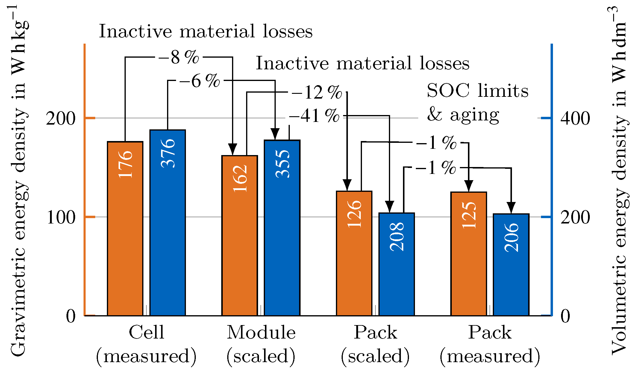
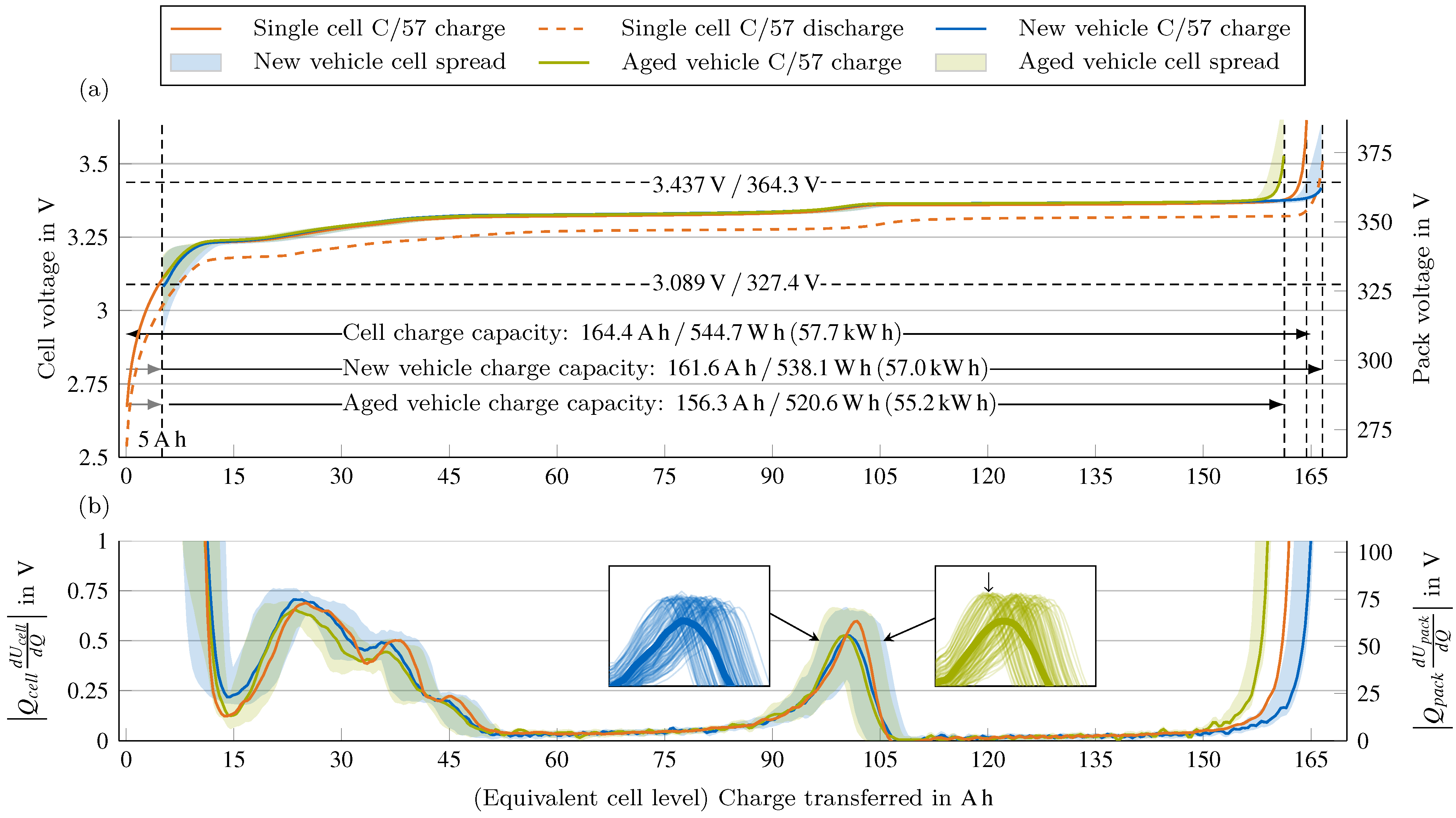
  • Component integration, energy density, and aging diagnosis.
    From 176 Wh/kg gravimetric and 376 Wh/L volumetric energy density on the cell level, the energy density drops down to 162 Wh/kg and 355 Wh/L on the module level and even further to 126 Wh/kg and 208 Wh/L on the battery pack level. If the voltage limit on the battery pack level is also considered, an additional 1% of energy density is lost. Transferring the DVA results from the cell level to the battery pack or vehicle level provides consistent results. This analysis enables aging observations in early states of calendric and cyclic aging.
  • Power unit efficiency.
    All tests on the chassis dynamometer were recorded with the vehicle set to dyno mode, which limits its power capabilities. For the installed LFP cells, the SOC only negligibly affected the power unit’s efficiency, as shown by differences in the efficiency map of low, middle (reference), and high SOC levels. The maximum efficiency of 97% in both maps is reached at high speeds of 12,000–16,000 1/min and rather low torques.
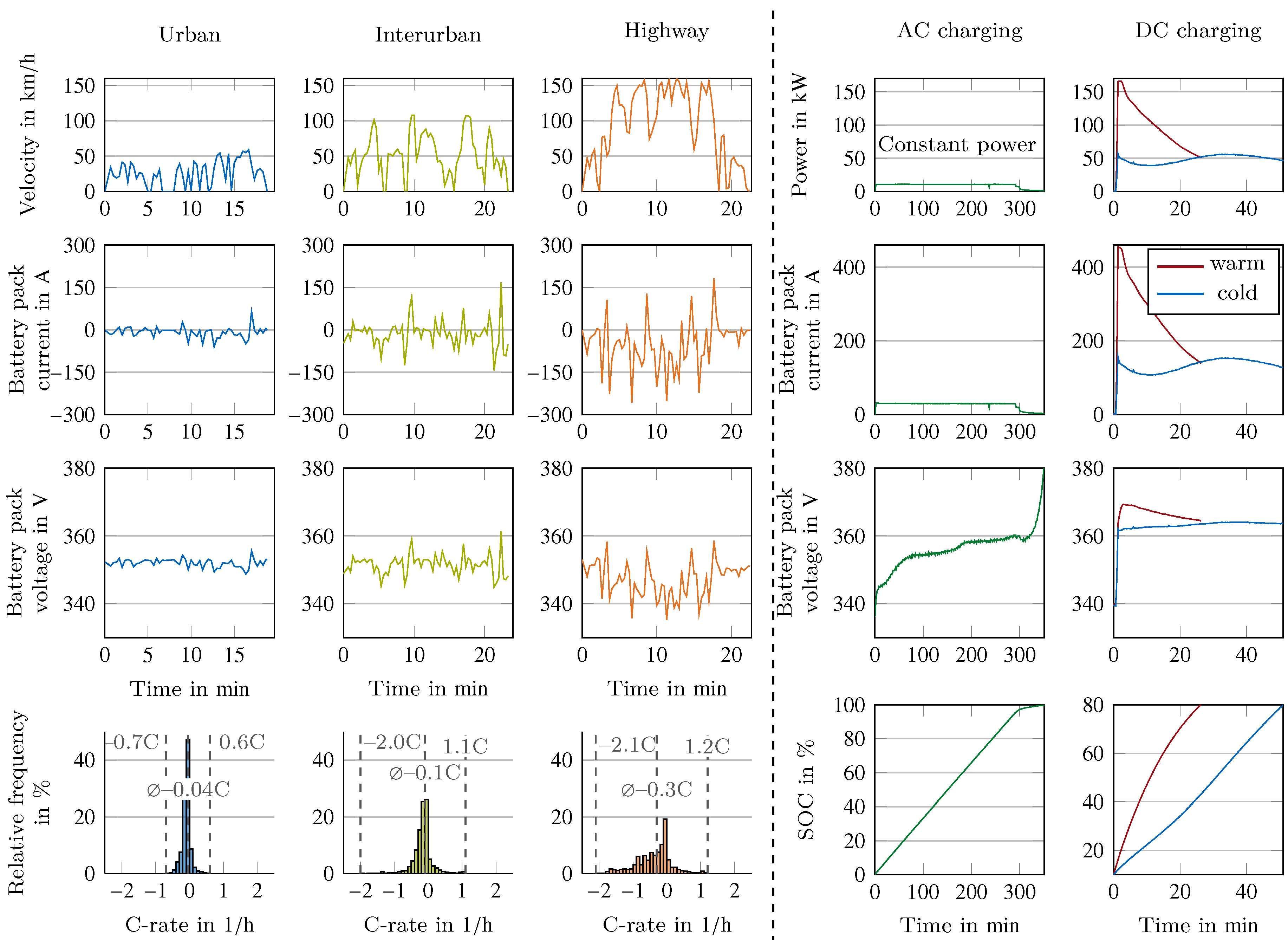
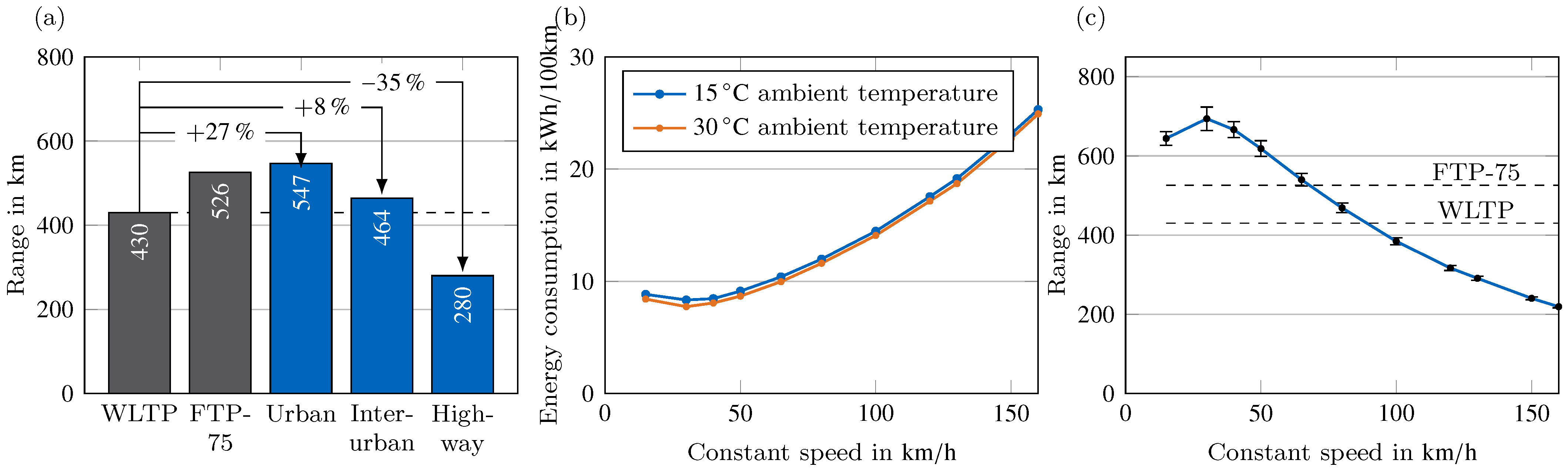
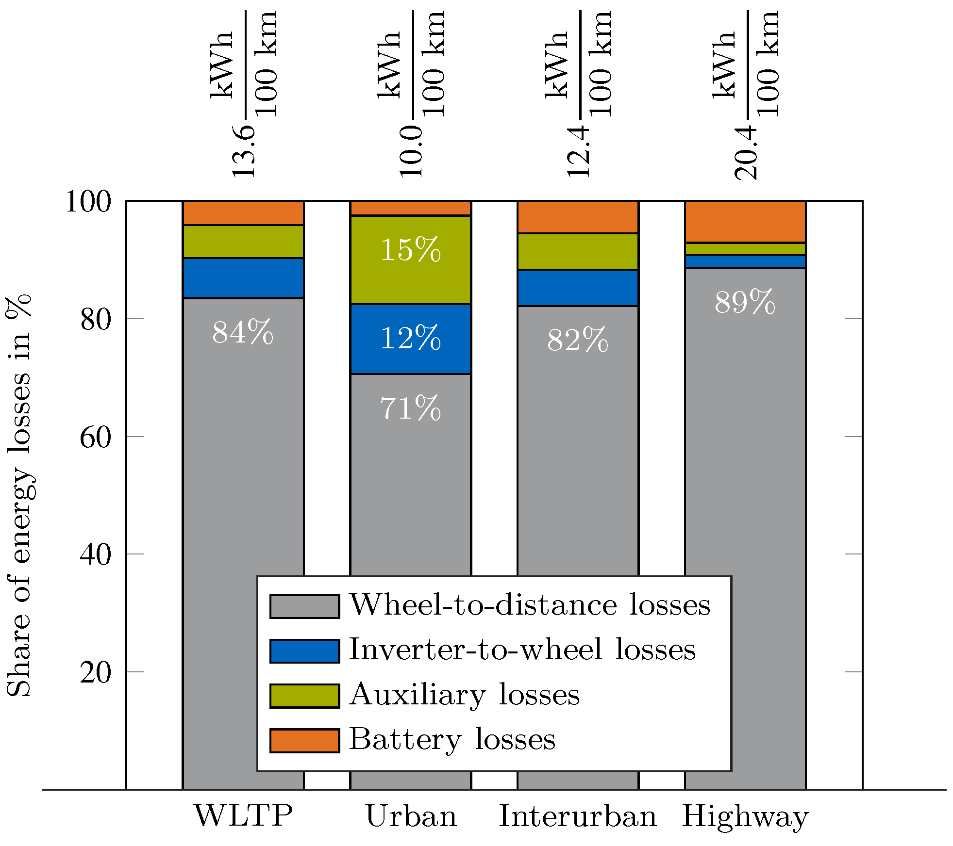
  • Range deviations from standard cycles.
    When comparing real-world driving scenarios to the official test procedures, the range of the urban (547 km) and interurban (464 km) drive cycles exceeds the range of the WLTP cycle (430 km), while only the urban cycle exceeds the Federal Test Procedure (FTP-75) cycle’s range (526 km). Due to aerodynamic losses, the highway cycle (280 km) reaches the lowest achievable electric range, even though the power unit reaches the highest possible efficiency at high speeds. Comparing the different shares of energy losses, the wheel-to-distance losses appear to reach the highest shares (between 71% and 89%), with other losses in similar shares in the respective drive cycles depending on the vehicle’s velocity. The electric range during real-world usage could be improved either by adjusting the areas of highest efficiency closer to those regions that are mainly driven, or by enhancing the current regenerative braking control logic, which might be set too conservatively regarding potential lithium plating of the LFP cells. This latter was observed during the braking test series, in which the brake pedal did not impact the share of regenerative braking. Although this is connected to more tuning effort, increasing the electric braking shares during brake pedal activation would increase the vehicle’s efficiency. Depending on the current vehicle state, a more advanced control strategy that distinguishes between different driving and charging modes might further improve the vehicle’s range.
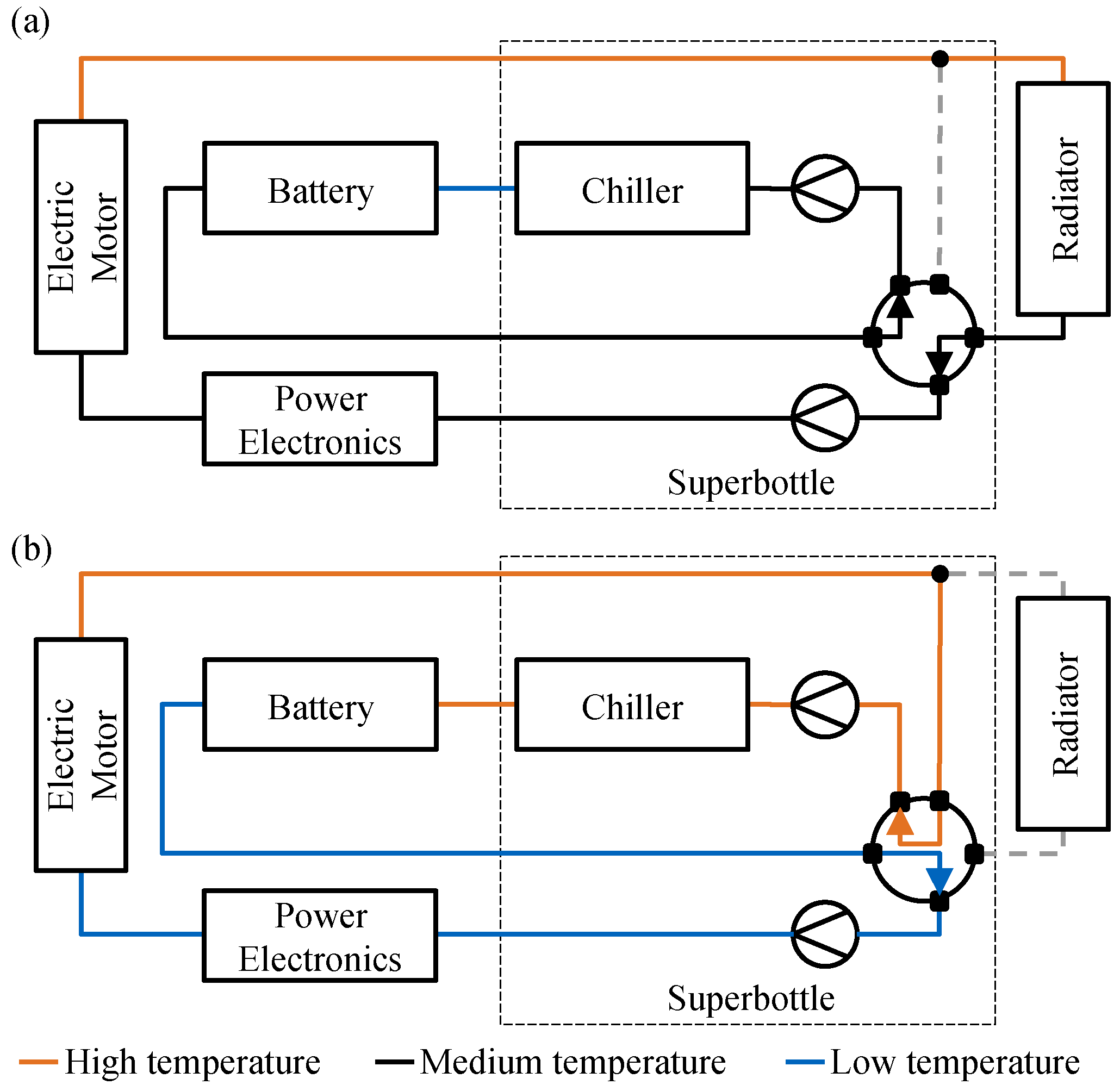
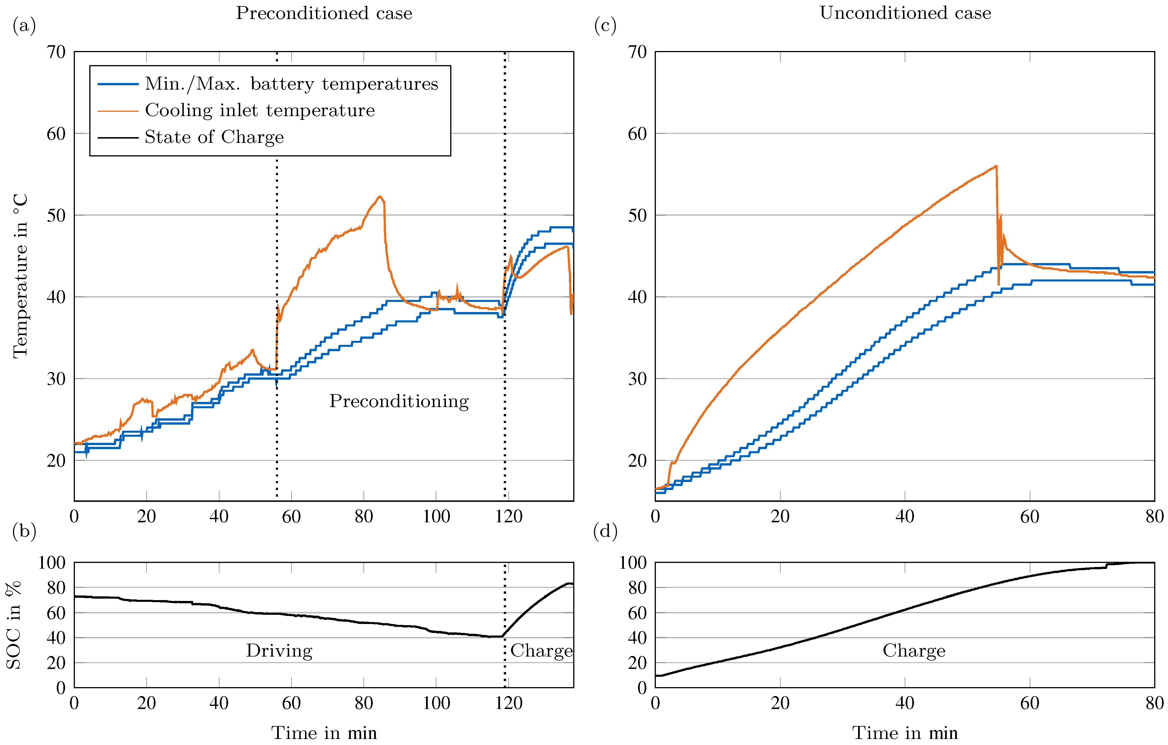
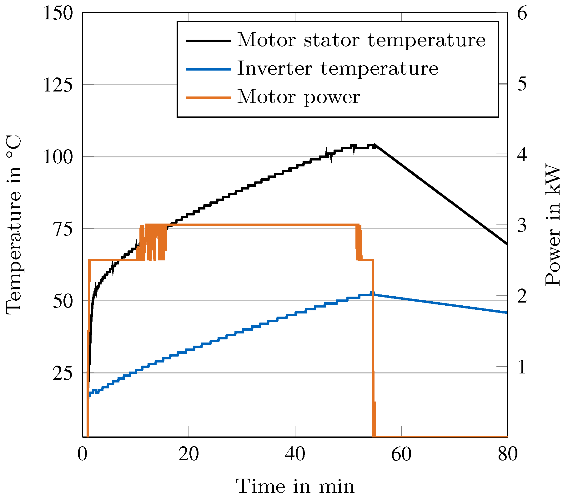
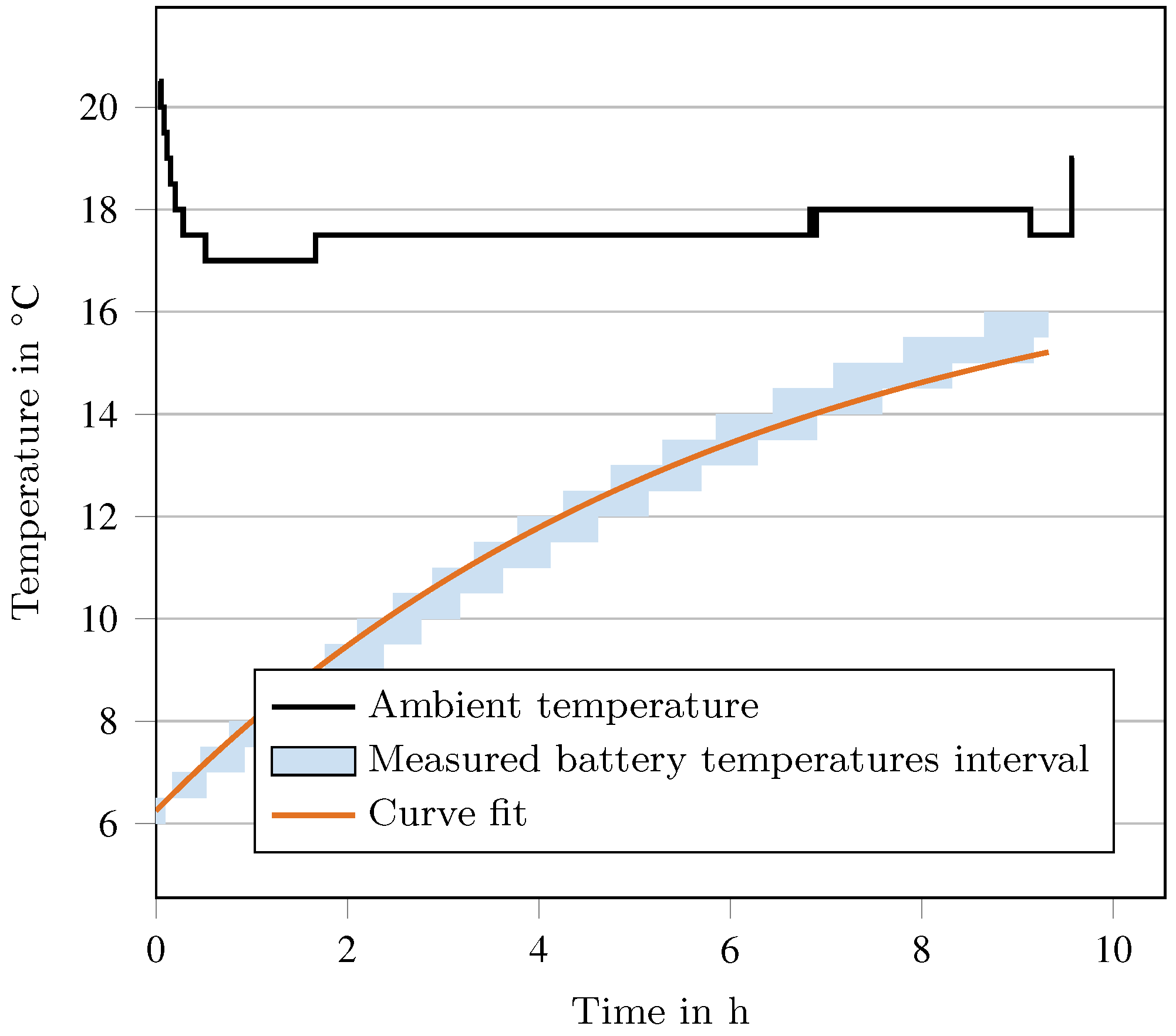
  • Thermal management of the battery pack.
    A maximal thermal gradient between the battery modules of 2 K while driving within the highway scenario and 3.5 K during fast charging with an active chiller cooling was measured. During battery heating, a maximum spread of 3 K occurs. The threshold of 5 K from the literature was not exceeded in any of the investigated scenarios, underlining the importance of temperature homogeneity for the battery’s performance and lifetime. When parking at low ambient temperatures, fast cool-down of the battery pack can be observed. Therefore, active battery heating is required, which is realized by serial connection between the electric motor and the battery within the cooling circuit. The heating power is provided by the generation of up to 3 kW additional power losses in the electric motor. Our investigation of the charging protocols shows that fast charging is targeted at battery surface temperatures between 40 °C to 50 °C, which is also advised in literature, where a maximum of 60 °C is stated. The battery heating preconditioning starts one hour prior to reaching the targeted charging station. During the charging process, the battery is cooled to stay below 50 °C. The presented thermal management strategies could be optimized using intelligent automated self-learning strategies to reduce charging times and extend the battery’s lifetime.

Author Contributions

N.R.: conceptualization, methodology, investigation, resources, writing —original draft, visualization, writing—review and editing, project administration. N.R. is the first author. P.R.: investigation, writing—original draft, writing—review and editing, visualization. P.B.: investigation, writing—original draft, writing—review and editing, visualization. J.S. (Jan Schöberl): investigation, writing—original draft, writing—review and editing, visualization. O.T.: investigation, writing—original draft, writing—review and editing, visualization. J.S. (Jakob Schneider): investigation, writing—original draft, writing—review and editing, visualization. K.A.G.: investigation, writing—original draft, writing—review and editing, visualization. C.A.: investigation, writing—original draft, writing—review and editing, visualization. B.D.: investigation, writing—original draft, writing—review and editing, visualization. M.S.: investigation, writing—review and editing, visualization. M.A.: investigation, writing—review and editing, visualization. T.K.: investigation, writing—review and editing, visualization, data curation. A.K.: investigation, writing—review and editing, visualization. M.L.: resources, supervision, writing—review and editing, funding acquisition. All authors have read and agreed to the published version of the manuscript.

Funding

This project has been partly funded by the German Federal Ministry for Economic Affairs and Climate Action (BMWK) within the projects “ScaleUp-eDrive” under grant number 16THB0006C, “NEFTON” under grant number 01MV21004A, and “ultraBatt” under grant number 01MV21015D; partly funded by the German Federal Ministry of Education and Research (BMBF) within the projects “BALd” under grant number 03XP0320B, “BetterBat” under grant number 03XP0362C, “OptiPro” under grant number 03XP0364B, “ComfficientShare” under grant number 03ZU1105CA, and “TUBE” under grant number 03XP0425; and partly funded by the Bavarian Ministry of Economic Affairs and Information and Communication Technology program within the projects ”charge.COM” under grant number DIK-0262/02 and “KiBaTest” under grant number DIK-0123/01.

Data Availability Statement

The original data presented in the study are available as open source via mediaTUM: https://doi.org/10.14459/2024mp1735494. Also, data of 228 individual real-world driving situations is accesible via mediaTUM: https://doi.org/10.14459/2024mp1735471.

Conflicts of Interest

The authors declare no conflicts of interest.

Appendix A. Vehicle Specifications

The vehicle specifications of the vehicle under study are provided in Table A1.
Table A1. Overview of vehicle specifications of the Tesla Model 3 under study. Data are collected from the Certificate of Conformity (COC) according to EU Regulation 2018/858 [29], vehicle registration documents, previous material analysis of the battery cell [75], and assumptions based on media and press releases.
DomainAttributeValueUnit
VehicleRange (WLTP) c440km
Max. speed c225km/h
Mass c1825 kg
Actual mass c1861 kg
Tyres c235/45R18 98Y-
Tyre radius m346.8mm
load coefficient—f0 c149.92N
load coefficient—f1 c0.6299N/(km/h)
load coefficient—f2 c0.02482N/(km/h)2
Power unitMax. power c239kW
30 min power c100kW
Max. rotations a16,0001/min
Max. torque r420Nm
Drive type aSyn-RM
Inverter aMOSFET
Gearing ratio c9.04:1-
Battery unitPack energy r58kWh
Cell capacity l161.2Ah
Cell format lprismatic-
Chemistry lLFP-
m Determined by measurements c Taken from the Certificate of Conformity (COC) r Taken from the vehicle registration documents l Taken from the literature, i.e., [75] a Assumptions taken from media and press releases.

Appendix B. Coast-Down Procedure and Driving Resistance Regressions

The coast-down procedure was performed multiple times to ensure statistical safety by reducing the impact of irregularities on the road surface. Every run was repeated three times in both directions for every speed level. The remaining deviations are explained by the test track, or rather by its unevenness and slope on the one hand and by the subdivided speed levels routed in the shortness of the test track on the other. These deviations lead to curvature errors, considering that the dynamometer does not consider slopes when simulating the results from the test track. Figure A1a shows the results from the coast-down procedure on the test track against the simulations on the chassis dynamometer. Evaluating the results from the test track, the target coefficients of the vehicle are determined to be a 0 = 177.205   N ,   a 1 = 5.743   N / ( m / s ) and a 2 = 0.254   N / ( m / s ) 2 . Transferring the parameters of real driving behavior on the dynamometer while considering its resistances, the parameters were adjusted iteratively until both curves could be superposed with an acceptable error. The closest parameter set meeting the results of the test track was achieved by a 0 = 65.0   N ,   a 1 = 4.09   N / ( m / s ) and a 2 = 0.254   N / ( m / s ) 2 with an RMSE of 0.67 km/h.
Figure A1. Coast-down measurements. (a) Coast-down velocity over time measured on the test track and on the dynamometer. (b) Driving resistance measured on the test track compared to data from the Certificate of Conformity (CoC) and data from the Environmental Protection Agency (EPA).
Wevj 15 00268 g0a1
Figure A1b compares the experimentally conducted coast-down curve to the parameters in the CoC provided in Table A1. In addition to the parameters provided by the manufacturer, the coast-down curve of the Environmental Protection Agency (EPA) is included with the parameters of a 0 = 134.8   N ,   a 1 = 2.12   N / ( m / s ) and a 2 = 0.283   N / ( m / s ) 2 [75]. Both curves present clear deviations from the officially provided coast-down curve, especially the measured curve in the lower speed range (which might be explained by the uneven road surface of the test track and optimal boundary conditions during the manufacturer’s test) and the EPA-curve in higher speed ranges. Comparing these results to the ones of the dynamometer range tests, the deviations are considered acceptable.

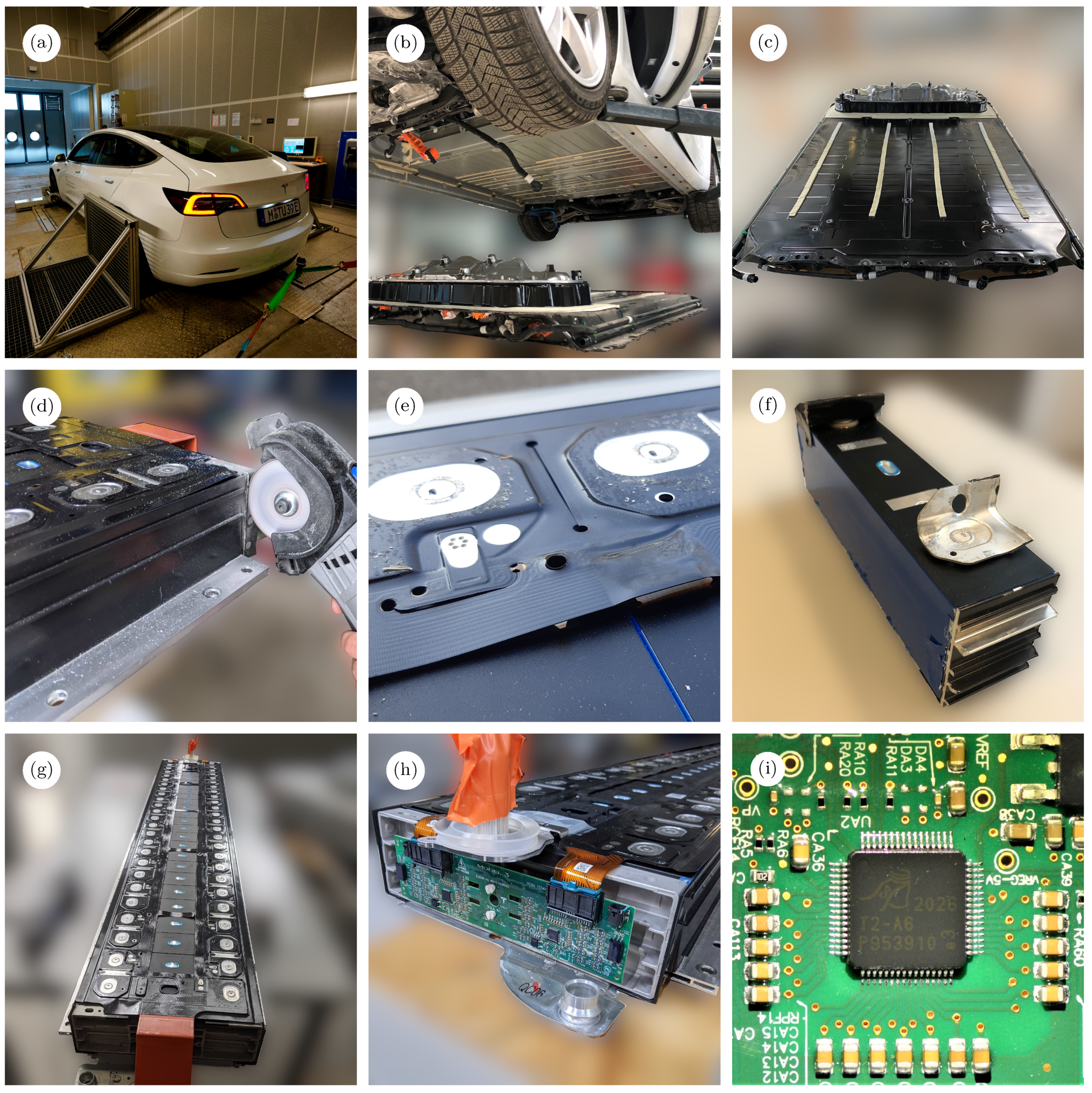
Appendix C. Battery Pack Teardown

As shown in Figure A2b, we removed the battery pack from the vehicle in order to gather information about its geometry and mass. Contrary to many other BEVss, such as the VW ID.3 [15], it is secured with threaded fasteners from both the bottom and top, requiring partial disassembly of interior components. Figure A2c shows the entire battery pack, the coolant lines around it, and the “penthouse” hump in the rear housing, which contains the BMS, the DC–DC converter feeding the 12 V system, and the onboard AC–DC converter for charging. Indents in the pack’s upper cover indicate the internal structure of four side-by-side longitudinal modules, each containing one row of hardcase prismatic cells. While the outer two are configured as 25s1p modules, the longer inner ones possess three more cells each, resulting in a 28s1p configuration. All modules are connected in series, leading to a 106s1p pack configuration. The cells have a nominal capacity and voltage of 161 A h and 3.2 V, respectively [76], leading to a nominal pack energy content and voltage of 54.6 kW h and 339.2 V. For further assessment on lower integration levels, an entire outer module was acquired from a torn-down equivalent vehicle of unknown mileage and disassembled for cell testing.
Structurally, the module braces (and presumably pre-tensions) its cells using one extruded L-shaped aluminum beam on either side, which are covered in black adhesive foil and stiffened by multiple fins. They are held together by two cast-aluminum end caps connected with three rivets at each corner and glued to the cells. The separation of the end caps from the beams during teardown is shown in Figure A2d. Further pre-tension is achieved by a 3.5 mm thick (in a compressed state) white foam material in between each end cap and cell stack. The two bracing beams of our small type module are not mirrored, with the one on the outer side of the pack having a considerably larger bare aluminum rib (Figure A2d) used to bolt the module down in the pack and the inner one interfacing with a longitudinal spar in the pack structure. The lower arm of the L-shaped beams secures the aluminum cooling plate to the cell stack, which contains six parallel coolant channels (trapezoid cross-section: ca. 15 mm by 3 mm each) ending in one pipe connector orificed to a diameter of 10 mm on either end. The channels are not evenly distributed across the cooling plate’s width, instead being arranged in two sets of three below the cells’ terminal areas. The thermal connection is established by a 0.5 mm thick green liquid resin applied to the mating face and cured to a hard state. Two spacer strips between the mating surfaces ensure a constant resin thickness. The cells’ thin bare aluminum cases are individually wrapped in multiple layers of blue adhesive foil on the sides and bottom. At the same time, the top is covered in black electrically insulating material, except for the functional surfaces described later and visible in Figure A2f.
Electrically, the cells are connected to each other using 54 mm wide and 1.5 mm thick aluminum bus bars, which are laminated in multifunctional black plastic wrapping except for the mating and welding surfaces. A further plastic insulator is lightly glued onto the laminate after welding, covering these open electrical points. All but of the one bus bars have narrow points (minimum width 47.5 mm) in between the cell terminals, while the one between cells 17 and 18 (counting from the negative module end) features an orifice of four separate prongs, each 3.3 mm wide, of uncertain function. This is probably designed as an emergency fuse, as there is no second voltage sense point for it, which would be required for a current shunt. The cells and bus bars are 12.7 mm, ring-shaped, and laser welded, with a weld line of width approximately 2.6 mm on top. While the laminated wrapping ensures proper positioning of all bars prior to module assembly and enables simultaneous welding processes on multiple cells, it also integrates the voltage and temperature sensors and wiring, which is done using flexible printed circuit (FCP) technology. The voltage sense lines end in a metal strip, one of which is spot-welded (with the spots arranged in a hexagon) to every bus bar, as shown in Figure A2e. The FCP wires end in connectors on the positive end of the module, leading into the BMS PCB. Three temperature sensors are present in the module on top of the first, third, and last cells (counting from the negative end). These are covered by glass fiber reinforced plastic (GFRP) stiffening plates laminated into the wrapping and connected using mint-green thermal pads onto off-center bare points of the cells’ top surface on either side of the vent hole (visible without a thermal pad in Figure A2f). Each cell features a centrally positioned oval pressure relief valve (23 mm by 13 mm) on top.
Figure A2. Test and tear-down procedures. (a) Vehicle under test on a chassis dynamometer. (b,c) Battery pack outside the vehicle. (d) Module teardown procedure. (e) Laminated cell terminal bus bars, including voltage sense and wiring. (f) Single cell prepared for testing. (g) Module under investigation. (h) BMS PCB of a module. (i) Microcontroller on PCB of the module’s BMS.
Wevj 15 00268 g0a2
The BMS PCB of the investigated module has a size of 232 mm by 60 mm and is mounted on the front side of the module in a vertical position as displayed in Figure A2h. A detailed view of the PCB is provided in Figure A3 in Appendix D. As two connection pins on the PCB are labeled “ISOSPI-A-N” and “ISOSPI-A-P”, the communication protocol used for the microcontroller is ISOSPI.
The layout of the PCB is divided into two similar setups, one for each connector to the FCP wires. In addition to other components, the setups consist of several identical resistor groups. The numbering of the resistor setups starts at 0 and runs up to 28, with setup number 14 found in the setups of both connectors. Regarding the doubled setup for index 14, this results in a total number of resistor setups of 30. As described by Samaddar et al. [77], a passive balancing circuit for n cells usually requires n + 1 resistors. Assuming that both setups contain a separate balancing circuit for n A (respectively, n B ) cells, the total number of resistors n resistors for a total of n A + n B = 25 cells is computed to be n resistors = ( n A + 1 ) + ( n B + 1 ) = 27 , which does not match the 30-resistor setups found on the PCB. Due to the battery pack’s inhomogeneous module size, it is assumed that the same BMS PCB is used for both module sizes, as the larger 28-cell module satisfies the equation for 30 resistors.

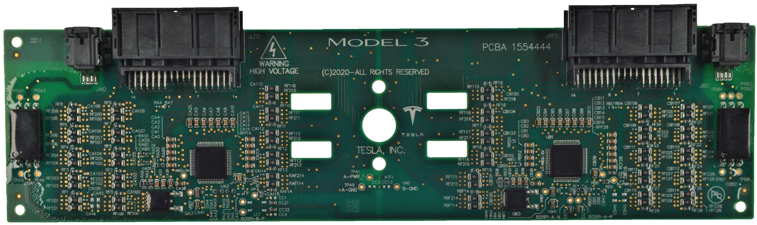
Appendix D. Printed Circuit Board of the Battery Management System of the Module Under Investigation

The PCB described in Appendix C was detached from the investigated battery module, which is illustrated in Figure A3.
Figure A3. PCB of the BMS of the 25 cell module under investigation.
Wevj 15 00268 g0a3

References

  1. International Energy Agency. Global EV Outlook 2023; International Energy Agency: Paris, France, 2023. [Google Scholar]
  2. European Union Council. Regulation (EU) 2021/1119 of the European Parliament and of the Council of 30 June 2021 Establishing the Framework for Achieving Climate Neutrality and Amending Regulations (EC) No 401/2009 and (EU) 2018/1999 (‘European Climate Law’); European Union Council: Brussels, Belgium, 2021. [Google Scholar]
  3. European Environment Agency. Transport and Environment Report 2021: Decarbonising Road Transport—The Role of Vehicles, Fuels and Transport Deman; European Environment Agency: Brussels, Belgium, 2021. [Google Scholar] [CrossRef]
  4. European Commission. Delivering the European Green Deal; European Commission: Brussels, Belgium, 2022. [Google Scholar]
  5. Allinson, M. How have electric cars advanced in the past 10 years and what’s the future? In Robotics Automation News; European Commission: Brussels, Belgium, 2023. [Google Scholar]
  6. König, A.; Nicoletti, L.; Schröder, D.; Wolff, S.; Waclaw, A.; Lienkamp, M. An Overview of Parameter and Cost for Battery Electric Vehicles. World Electr. Veh. J. 2021, 12, 21. [Google Scholar] [CrossRef]
  7. van Mierlo, J.; Berecibar, M.; El Baghdadi, M.; de Cauwer, C.; Messagie, M.; Coosemans, T.; Jacobs, V.A.; Hegazy, O. Beyond the State of the Art of Electric Vehicles: A Fact-Based Paper of the Current and Prospective Electric Vehicle Technologies. World Electr. Veh. J. 2021, 12, 20. [Google Scholar] [CrossRef]
  8. Blomgren, G.E. The Development and Future of Lithium Ion Batteries. J. Electrochem. Soc. 2017, 164, A5019–A5025. [Google Scholar] [CrossRef]
  9. Momen, F.; Rahman, K.; Son, Y. Electrical propulsion system design of Chevrolet Bolt battery electric vehicle. IEEE Trans. Ind. Appl. 2018, 55, 376–384. [Google Scholar] [CrossRef]
  10. Sarlioglu, B.; Morris, C.T.; Han, D.; Li, S. Benchmarking of electric and hybrid vehicle electric machines, power electronics, and batteries. In Proceedings of the 2015 Intl Aegean Conference on Electrical Machines & Power Electronics (ACEMP), 2015 Intl Conference on Optimization of Electrical & Electronic Equipment (OPTIM) & 2015 Intl Symposium on Advanced Electromechanical Motion Systems (ELECTROMOTION), Online, 2–4 September 2015; pp. 519–526. [Google Scholar] [CrossRef]
  11. Kovachev, G.; Schröttner, H.; Gstrein, G.; Aiello, L.; Hanzu, I.; Wilkening, H.; Foitzik, C.; Wellm, M.; Sinz, W.; Ellersdorfer, C. Analytical Dissection of an Automotive Li-Ion Pouch Cell. Batteries 2019, 5, 67. [Google Scholar] [CrossRef]
  12. Löbberding, H.; Wessel, S.; Offermanns, C.; Kehrer, M.; Rother, J.; Heimes, H.; Kampker, A. From Cell to Battery System in BEVs: Analysis of System Packing Efficiency and Cell Types. World Electr. Veh. J. 2020, 11, 77. [Google Scholar] [CrossRef]
  13. Oh, G.; Leblanc, D.J.; Peng, H. Vehicle Energy Dataset (VED), A Large-Scale Dataset for Vehicle Energy Consumption Research. IEEE Trans. Intell. Transp. Syst. 2020, 11, 23. [Google Scholar] [CrossRef]
  14. Diez, J. Advanced Vehicle Testing and Evaluation, Final Technical Report Encompassing Project Activities from 1 October 2011 to 30 April 2018; Technical Report; Intertek Testing Services, NA, Inc.: Arlington, IL, USA, 2018. [Google Scholar]
  15. Wassiliadis, N.; Steinsträter, M.; Schreiber, M.; Rosner, P.; Nicoletti, L.; Schmid, F.; Ank, M.; Teichert, O.; Wildfeuer, L.; Schneider, J.; et al. Quantifying the state of the art of electric powertrains in battery electric vehicles: Range, efficiency, and lifetime from component to system level of the Volkswagen ID.3. eTransportation 2022, 12, 100167. [Google Scholar] [CrossRef]
  16. Lancelot, J.; Rimal, B.P.; Dennis, E.M. Performance Evaluation of a Lane Correction Module Stress Test: A Field Test of Tesla Model 3. Future Internet 2023, 15, 138. [Google Scholar] [CrossRef]
  17. Xu, B.; Arjmandzadeh, Z. Parametric study on thermal management system for the range of full (Tesla Model S)/ compact-size (Tesla Model 3) electric vehicles. Energy Convers. Manag. 2023, 278, 116753. [Google Scholar] [CrossRef]
  18. Ank, M.; Sommer, A.; Gamra, K.A.; Schöberl, J.; Leeb, M.; Schachtl, J.; Streidel, N.; Stock, S.; Schreiber, M.; Bilfinger, P.; et al. Lithium-Ion Cells in Automotive Applications: Tesla 4680 Cylindrical Cell Teardown and Characterization. J. Electrochem. Soc. 2023, 170, 120536. [Google Scholar] [CrossRef]
  19. Statista.com. Best-Selling Plug-in Electric Vehicle Models Worldwide in 2022. 2023. Available online: https://www.statista.com (accessed on 14 February 2023).
  20. EV Specifications. 2017 Tesla Model 3 Long Range RWD—Specifications; Hearst Autos Inc.: Chamblee, GA, USA, 2022. [Google Scholar]
  21. EV Specifications. 2018 Tesla Model 3 Mid Range RWD—Specifications; Hearst Autos Inc.: Chamblee, GA, USA, 2022. [Google Scholar]
  22. EV Specifications. 2019 Tesla Model 3 Standard Range RWD—Specifications; Hearst Autos Inc.: Chamblee, GA, USA, 2022. [Google Scholar]
  23. EV Specifications. 2019 Tesla Model 3 Standard Range Plus RWD—Specifications; Hearst Autos Inc.: Chamblee, GA, USA, 2022. [Google Scholar]
  24. EV Specifications. 2023 Tesla Model 3 RWD—Specifications; Hearst Autos Inc.: Chamblee, GA, USA, 2022. [Google Scholar]
  25. EV Specifications. 2021 Tesla Model 3 Long Range AWD—Specifications and Price; Hearst Autos Inc.: Chamblee, GA, USA, 2022. [Google Scholar]
  26. EV Specifications. 2021 Tesla Model 3 Performance AWD—Specifications and Price; Hearst Autos Inc.: Chamblee, GA, USA, 2022. [Google Scholar]
  27. InsideEVs. Tesla Now Has Multiple Battery Options: Which One Should You Choose? Hearst Autos Inc.: Chamblee, GA, USA, 2022. [Google Scholar]
  28. ISO 1176:1990-07; Road Vehicles—Masses—Vocabulary and Codes. International Organization for Standardization: Geneva, Switzerland, 1990.
  29. European Parliament. Regulation (EU) 2018/858 of the European Parliament and of the Council of 30 May 2018 on the Approval and Market Surveillance of Motor Vehicles and Their Trailers, and of Systems, Components and Separate Technical Units Intended for such Vehicles, Amending Regulations (EC) No. 715/2007 and (EC) No. 595/2009 and Repealing Directive 2007/46/EC; European Parlament: Strasbourg, France, 2018. [Google Scholar]
  30. Wardell, J. Model3dbc. Available online: https://github.com/joshwardell/model3dbc (accessed on 14 February 2023).
  31. Barai, A.; Uddin, K.; Dubarry, M.; Somerville, L.; McGordon, A.; Jennings, P.; Bloom, I. A comparison of methodologies for the non-invasive characterisation of commercial Li-ion cells. Prog. Energy Combust. Sci. 2019, 72, 1–31. [Google Scholar] [CrossRef]
  32. Lewerenz, M.; Marongiu, A.; Warnecke, A.; Sauer, D.U. Differential voltage analysis as a tool for analyzing inhomogeneous aging: A case study for LiFePO4-Graphite cylindrical cells. J. Power Sources 2017, 368, 57–67. [Google Scholar] [CrossRef]
  33. Fath, J.P.; Dragicevic, D.; Bittel, L.; Nuhic, A.; Sieg, J.; Hahn, S.; Alsheimer, L.; Spier, B.; Wetzel, T. Quantification of aging mechanisms and inhomogeneity in cycled lithium-ion cells by differential voltage analysis. J. Energy Storag. 2019, 25, 100813. [Google Scholar] [CrossRef]
  34. Dubarry, M.; Devie, A.; Liaw, B.Y. The value of battery diagnostics and prognostics. Energy Power Sources 2014, 1, 242–249. [Google Scholar]
  35. Pütz, R.; Serne, T. Rennwagentechnik—Praxislehrgang Fahrdynamik, 1st ed.; Springer: Wiesbaden, Germany, 2017. [Google Scholar] [CrossRef]
  36. Liebl, J.; Lederer, M.; Rohde-Brandenburger, K.; Biermann, J.W.; Roth, M.; Schäfer, H. Energiemanagement im Kraftfahrzeug, 1st ed.; Springer Vieweg: Wiesbaden, Germany, 2014. [Google Scholar] [CrossRef]
  37. The European Comission. Comission Regulation (EU) 2018/1832; The European Comission: Geneva, Switzerland, 2018. [Google Scholar]
  38. Gyenes, B.; Stevens, D.A.; Chevrier, V.L.; Dahn, J.R. Understanding Anomalous Behavior in Coulombic Efficiency Measurements on Li-Ion Batteries. J. Electrochem. Soc. 2015, 162, A278–A283. [Google Scholar] [CrossRef]
  39. Petzl, M.; Danzer, M.A. Advancements in OCV Measurement and Analysis for Lithium-Ion Batteries. IEEE Trans. Energy Convers. 2013, 28, 675–681. [Google Scholar] [CrossRef]
  40. Simolka, M.; Heger, J.F.; Traub, N.; Kaess, H.; Friedrich, K.A. Influence of Cycling Profile, Depth of Discharge and Temperature on Commercial LFP/C Cell Ageing: Cell Level Analysis with ICA, DVA and OCV Measurements. J. Electrochem. Soc. 2020, 167, 110502. [Google Scholar] [CrossRef]
  41. Noel, M.; Santhanam, R. Electrochemistry of graphite intercalation compounds. J. Power Sources 1998, 72, 53–65. [Google Scholar] [CrossRef]
  42. Aurbach, D.; Markovsky, B.; Weissman, I.; Levi, E.; Ein-Eli, Y. On the correlation between surface chemistry and performance of graphite negative electrodes for Li ion batteries. Electrochim. Acta 1999, 45, 67–86. [Google Scholar] [CrossRef]
  43. Winter, M.; Besenhard, J.O.; Spahr, M.E.; Novák, P. Insertion Electrode Materials for Rechargeable Lithium Batteries. Adv. Mater. 1998, 10, 725–763. [Google Scholar] [CrossRef]
  44. Lerf, A. Storylines in intercalation chemistry. Dalton Trans. 2014, 43, 10276–10291. [Google Scholar] [CrossRef] [PubMed]
  45. Keil, P.; Jossen, A. Calendar Aging of NCA Lithium-Ion Batteries Investigated by Differential Voltage Analysis and Coulomb Tracking. J. Electrochem. Soc. 2017, 164, A6066–A6074. [Google Scholar] [CrossRef]
  46. Keil, P.; Schuster, S.F.; Wilhelm, J.; Travi, J.; Hauser, A.; Karl, R.C.; Jossen, A. Calendar Aging of Lithium-Ion Batteries. J. Electrochem. Soc. 2016, 163, A1872–A1880. [Google Scholar] [CrossRef]
  47. Sarasketa-Zabala, E.; Gandiaga, I.; Rodriguez-Martinez, L.M.; Villarreal, I. Calendar ageing analysis of a LiFePO4/graphite cell with dynamic model validations: Towards realistic lifetime predictions. J. Power Sources 2014, 272, 45–57. [Google Scholar] [CrossRef]
  48. Li, D.; Danilov, D.L.; Gao, L.; Yang, Y.; Notten, P.H.L. Degradation Mechanisms of the Graphite Electrode in C6/LiFePO4 Batteries Unraveled by a Non-Destructive Approach. J. Electrochem. Soc. 2016, 163, A3016–A3021. [Google Scholar] [CrossRef]
  49. Dubarry, M.; Anseán, D. Best practices for incremental capacity analysis. Front. Energy Res. 2022, 10, 555. [Google Scholar] [CrossRef]
  50. Schaltz, E.; Norregaard, K.; Christensen, A. Incremental Capacity Analysis Applied on Electric Vehicles for Battery State-of-Health Estimation. In Proceedings of the 2019 Fourteenth International Conference on Ecological Vehicles and Renewable Energies (EVER), Monte-Carlo, Monaco, 8–10 May 2019. [Google Scholar]
  51. Schaltz, E.; Stroe, D.I.; Norregaard, K.; Ingvardsen, L.S.; Christensen, A. Incremental Capacity Analysis Applied on Electric Vehicles for Battery State-of-Health Estimation. IEEE Trans. Ind. Appl. 2021, 57, 1810–1817. [Google Scholar] [CrossRef]
  52. Weng, C.; Feng, X.; Sun, J.; Peng, H. State-of-health monitoring of lithium-ion battery modules and packs via incremental capacity peak tracking. Appl. Energy 2016, 180, 360–368. [Google Scholar] [CrossRef]
  53. Nicoletti, L. Parametric Modeling of Battery Electric Vehicles in the Early Development Phase. Ph.D. Thesis, Technical University of Munich, Munich, Germany, 2022. [Google Scholar]
  54. EV Database. Tesla Model 3 Standard Plus; EV Database: Amsterdam, The Netherlands, 2020. [Google Scholar]
  55. MotorBiscuit. Tesla Driving Mode Was so Dangerous that Tesla Disabled It; Tesla Company: San Carlos, CA, USA, 2022. [Google Scholar]
  56. Binder, A. Elektrische Maschinen und Antriebe: Grundlagen, Betriebsverhalten; Springer: Berlin/Heidelberg, Germany, 2012; pp. 617–619. [Google Scholar]
  57. Doppelbauer, M. Grundlagen der Elektromobilität: Technik, Praxis, Energie und Umwelt; Springer: Berlin/Heidelberg, Germany, 2020; pp. 48–200. [Google Scholar]
  58. Krull, J.T.; Pinto, P.M. Heating and Cooling Reservoir for a Battery Powered Vehicle. U.S. Patent 1,066,590,8B2, 26 May 2020. [Google Scholar]
  59. Yang, B.; Martins, T.V.; Graves, S.M.; Swint, E.; Bellemare, E.; Fedoseyev, L.; Dellal, B.; Olsen, L.E.; Hain, A. Electric Motor Waste Heat Mode to Heat Battery. U.S. Patent 1,121,804,5B2, 4 January 2022. [Google Scholar]
  60. Pesaran, A.A. Battery thermal models for hybrid vehicle simulations. J. Power Sources 2002, 110, 377–382. [Google Scholar] [CrossRef]
  61. Chung, Y.; Kim, M.S. Thermal analysis and pack level design of battery thermal management system with liquid cooling for electric vehicles. Energy Convers. Manag. 2019, 196, 105–116. [Google Scholar] [CrossRef]
  62. Wang, J.; Lu, S.; Wang, Y.; Li, C.; Wang, K. Effect analysis on thermal behavior enhancement of lithium–ion battery pack with different cooling structures. J. Energy Storage 2020, 32, 101800. [Google Scholar] [CrossRef]
  63. Yang, X.G.; Liu, T.; Gao, Y.; Ge, S.; Leng, Y.; Wang, D.; Wang, C.Y. Asymmetric Temperature Modulation for Extreme Fast Charging of Lithium-Ion Batteries. Joule 2019, 3, 3002–3019. [Google Scholar] [CrossRef]
  64. Yin, Y.; Choe, S.Y. Actively temperature controlled health-aware fast charging method for lithium-ion battery using nonlinear model predictive control. Appl. Energy 2020, 271, 115232. [Google Scholar] [CrossRef]
  65. Liu, T.; Ge, S.; Yang, X.G.; Wang, C.Y. Effect of thermal environments on fast charging Li-ion batteries. J. Power Sources 2021, 511, 230466. [Google Scholar] [CrossRef]
  66. Wassiliadis, N.; Schneider, J.; Frank, A.; Wildfeuer, L.; Lin, X.; Jossen, A.; Lienkamp, M. Review of fast charging strategies for lithium-ion battery systems and their applicability for battery electric vehicles. J. Energy Storage 2021, 44, 103306. [Google Scholar] [CrossRef]
  67. Tomaszewska, A.; Chu, Z.; Feng, X.; O’Kane, S.; Liu, X.; Chen, J.; Ji, C.; Endler, E.; Li, R.; Liu, L.; et al. Lithium-ion battery fast charging: A review. eTransportation 2019, 1, 100011. [Google Scholar] [CrossRef]
  68. Yang, X.G.; Liu, T.; Wang, C.Y. Thermally modulated lithium iron phosphate batteries for mass-market electric vehicles. Nat. Energy 2021, 6, 176–185. [Google Scholar] [CrossRef]
  69. Yang, X.G.; Wang, C.Y. Understanding the trilemma of fast charging, energy density and cycle life of lithium-ion batteries. J. Power Sources 2018, 402, 489–498. [Google Scholar] [CrossRef]
  70. Wassiliadis, N.; Abo Gamra, K.; Zähringer, M.; Schmid, F.; Lienkamp, M. Fast charging strategy comparison of battery electric vehicles and the benefit of advanced fast charging algorithms. In Proceedings of the Advanced Automotive Battery Conference, Detroit, MI, USA, 14–17 June 2022. [Google Scholar]
  71. Nobis, C.; Kuhnimhof, T. Mobilität in Deutschland- MiD: Ergebnisbericht; Bundesministerium für Verkehr und Digitale Infrastruktur: Bonn, Germany, 2018. [Google Scholar]
  72. Steinhardt, M.; Barreras, J.V.; Ruan, H.; Wu, B.; Offer, G.J.; Jossen, A. Meta-analysis of experimental results for heat capacity and thermal conductivity in lithium-ion batteries: A critical review. J. Power Sources 2022, 522, 230829. [Google Scholar] [CrossRef]
  73. Lienhard, I.V.J.H.; Lienhard, V.J.H. A Heat Transfer Textbook, 5th ed.; Dover Publications: Mineola, NY, USA, 2019. [Google Scholar]
  74. De Felice, M. Country Averages of Copernicus ERA5 Hourly Meteorological Variables; Zenodo: Geneva, Switzerland, 2018. [Google Scholar] [CrossRef]
  75. United States Environmental Protection Agency (EPA). Data on Cars Used for Testing Fuel Economy; EPA: New York, NY, USA, 2021.
  76. Contemporary Amperex Technology Ltd. Product Specifications—LFP6228082-161Ah; CATL: Ningde, China, 2023. [Google Scholar]
  77. Samaddar, N.; Kumar, N.S.; Jayapragash, R. Passive Cell Balancing of Li-Ion batteries used for Automotive Applications. J. Phys. Conf. Ser. 2020, 1716, 012005. [Google Scholar] [CrossRef]
Figure 1. Three real-world usage patterns measured during vehicle operation. Measured vehicle velocity, pack current, voltage, and load spectrum analysis for urban, interurban, and highway driving scenarios. Discharge sequences measured from 80% UI-SOC. Note that the grey dashed lines illustrate the minima, maxima, and arithmetic average of the underlying event. Pack power, current, and voltage for an 11 kW AC charge and 170 kW DC fast charge event. The DC fast charge event is split into operating temperature (red) and cold temperature (blue). AC charging between 0–100% UI-SOC. DC fast charging between 10–80% UI-SOC.
Wevj 15 00268 g001
Figure 2. Overview of the dimensions of the battery cell, module, and pack. All dimensions are indicated in mm. The drawings are not true to scale. For further geometrical information, the reader is referred to the reconstructed computer aided design (CAD) models in the supplementary materials provided alongside the article.
Wevj 15 00268 g002
Figure 3. Energy densities determined experimentally with C/57 CC charge sequences, weighing, and geometrical measurements at multiple integration levels.
Wevj 15 00268 g003
Figure 4. Thermodynamic battery behavior at C / 57 and 25(1) °C taken from both single cell (orange) and vehicle-level (blue/green) measurements. The right-hand side vertical axes are scaled by the number of cells in series to enable direct comparison between the vehicle-level measurements and left-hand side cell-level measurements. (a) The pOCV curves indicate the charge and energy throughput and the usable capacity on vehicle level. (b) The corresponding DVA curves; the ↓ indicates a number of cells shifted towards the left in the aged vehicle.
Wevj 15 00268 g004
Figure 5. Efficiency characteristics of the powertrain unit, inverter, and electric machine, created with discrete measurement points through recorded onboard data with estimated signals (i.e., motor torque). Base points are illustrated as crosses.
Wevj 15 00268 g005
Figure 6. Efficiency differences dependent on the SOC measured with software version 2022.20.8 (Figure 5b). (a) Low SOC level from 0–29% and (b) high SOC level from 61–100% compared to the reference model in the SOC range of 30–60%. Positive percentages stand for higher efficiencies compared to reference measurement.
Wevj 15 00268 g006
Figure 7. Experimentally determined travel distances. (a) Maximum achievable range in international test procedures compared to real-world cycles at an ambient temperature of 23 °C. (b) Experimentally determined energy consumption at constant speed levels with HVAC off. (c) Maximum achievable range at constant speed levels. Note that all experiments in (a) were been performed by continuously driving the vehicle until it could no longer follow the target velocity.
Wevj 15 00268 g007
Figure 8. Shares of different energy losses in the Tesla Model 3 for four driving cycles and total energy consumption.
Wevj 15 00268 g008
Figure 9. Cooling circuit, including the Superbottle. (a) In cooling mode, there are two separate cooling circuits. (b) In heating mode, the electric motor and the battery are connected in series to heat the battery.
Wevj 15 00268 g009
Figure 10. Thermal management engagement and temperature recordings of the battery pack and the cooling inlet. Δ T is calculated between the maximum and minimum temperature in the battery pack at each sample point. (a,b) Repeated highway cycle on the dynamometer and (c,d) DC fast charging event recorded at a 350 kW charging station.
Wevj 15 00268 g010
Figure 11. Fast charge processes at a 250 kW Ionity charger for a preconditioned battery when targeting a Tesla Supercharger within navigation compared to an unconditioned battery: (a,b) show the battery and cooling inlet temperature as well as the SOC for the conditioned case, while (c,d) display the unconditioned case.
Wevj 15 00268 g011
Figure 12. Motor stator and inverter temperature along with motor power during waste heat operation mode for battery heating while fast charging in the unconditioned case.
Wevj 15 00268 g012
Figure 13. Measurement and curve fit of Tesla Model 3 battery heating up to ambient temperature. The blue band is defined by the minimum and maximum measured battery temperatures.
Wevj 15 00268 g013
Figure 14. Battery temperature at the start of a trip for different initial temperatures after a range of parking durations at an ambient temperature of −8.5 °C.
Wevj 15 00268 g014
Figure 15. Single cell voltages and charging power during charging at an 11 kW wallbox to (a) 100% and (b) 88%. Each color represents a single cell. In (a), two deviating cell voltages and a switch from CP to CV charging are visible. Cell voltages during the relaxation phase in (b) clearly show noise-like behavior for approximately 40 min.
Wevj 15 00268 g015
Disclaimer/Publisher’s Note: The statements, opinions and data contained in all publications are solely those of the individual author(s) and contributor(s) and not of MDPI and/or the editor(s). MDPI and/or the editor(s) disclaim responsibility for any injury to people or property resulting from any ideas, methods, instructions or products referred to in the content.

