Abstract
This study provides a comprehensive simulation for understanding the influence of EV growth and its external factors on grid stability and offers insights into effective management strategies. To manage the growth of battery-based electric vehicles (BEVs) in Indonesia and mitigate their impact on the power grid’s supply–demand equilibrium, regulatory adjustments and subsidies can be implemented by the government. The Jawa-Madura-Bali (Jamali) electrical system, as the largest in Indonesia, is challenged with accommodating the rising number of vehicles. Following an analysis of Jamali’s electricity supply using data from the National Electricity Company (RUPTL), simulations are constructed to model the grid’s demand side. Input variables such as Jamali’s population, the numbers of internal combustion engine (ICE) and electric vehicles, initial charging times (ICT), slow and fast charging ratios, and BEV charge load curves are simulated. Scenario variables, including supply capacity growth rate, vehicle population growth rate, subsidy impact on EV attractiveness, ICT, and fast charging ratio, are subsequently simulated for the 2024–2029 period. Four key simulation outcomes are identified. The best-case scenario (scenario 1776) achieves the highest EV growth with minimal grid disruption, resulting in a 45.38% EV percentage in 2029 and requiring an annual allocation of 492 billion rupiah to match supply with demand. The worst-case scenario leads to a 23.12% EV percentage, necessitating 47,566 billion rupiah for EV subsidies in 2029. Additionally, the most and least probable scenarios based on the literature research are evaluated. This novel simulation and its results provide insights into EV growth’s impact on the grid’s balance in one presidential term from 2024 to 2029, aiding the government in planning regulations and subsidies effectively.
1. Introduction
Indonesia’s power system is one of the largest and most complex in Southeast Asia, characterized by its vast geographic spread across thousands of islands. The primary electricity provider is PLN (Perusahaan Listrik Negara, Jakarta, Indonesia), a state-owned enterprise that oversees the generation, transmission, and distribution of electricity. The power system is divided into several regional grids, with the Jawa-Bali grid being the largest and most significant, serving most of the population and industrial activities [1].
Indonesia is rapidly transitioning from internal combustion engine (ICE) vehicles to electric vehicles (EVs) to reduce dependency on imported fossil fuels, improve energy security, and meet climate goals. The shift will cut greenhouse gas emissions from the transportation sector and leverage Indonesia’s position as the world’s largest nickel producer, crucial for EV batteries. Government policies, incentives, and infrastructure development further support this swift transition to EVs.
As Indonesia transitions from ICE vehicles to EVs, ensuring the steady growth of BEVs is crucial to prevent disruption to the country’s power grid balance. Considering that the Jawa-Madura-Bali (Jamali) system constitutes Indonesia’s largest electrical system [1] and these islands accommodate the highest total number of vehicles [2], it is imperative to simulate the accelerated growth of electric vehicles to assess its impact.
The analysis of the Jamali electricity supply involves utilizing data from the National Electricity Company’s RUPTL [3]. Simulation of the grid’s demand side incorporates various input variables, including the Jamali population, populations of internal combustion engine (ICE) vehicles and electric vehicles (EVs), initial charging time (ICT), the ratio between slow and fast charging, and the charge load curve for each vehicle type. Moreover, scenario variables such as the rate of growth in supply capacity, vehicle population growth, the impact of subsidies on EV attractiveness, ICT, and the fast charging ratio are also simulated.
Following an examination of the data and simulations spanning the presidential period of 2024–2029, four prominent outcomes merit scrutiny: the best-case scenario, showcasing the most substantial EV growth while upholding the grid’s supply–demand equilibrium; the most probable scenario derived from extant literature; the least probable scenario; and the worst-case scenario.
The inputs of this simulation are adaptable to meet various requirements, and its outputs provide a framework for understanding the impact of EV growth on the grid’s supply –demand equilibrium from 2024 to 2029. By analyzing both the best- and worst-case scenario outcomes, the government can formulate regulations and subsidies accordingly.
This study aims to simulate the impact of EV growth on the grid’s stability from 2024 to 2029, considering various dynamic factors such as population growth and peak load variations. By leveraging data from RUPTL PLN and using MATLAB and Simulink for simulation, this research seeks to provide actionable insights into how to manage the increasing EV demand through effective policies or subsidies.
1.1. Jawa-Madura-Bali Power System (Grid Capacity and Peak Load Demand)
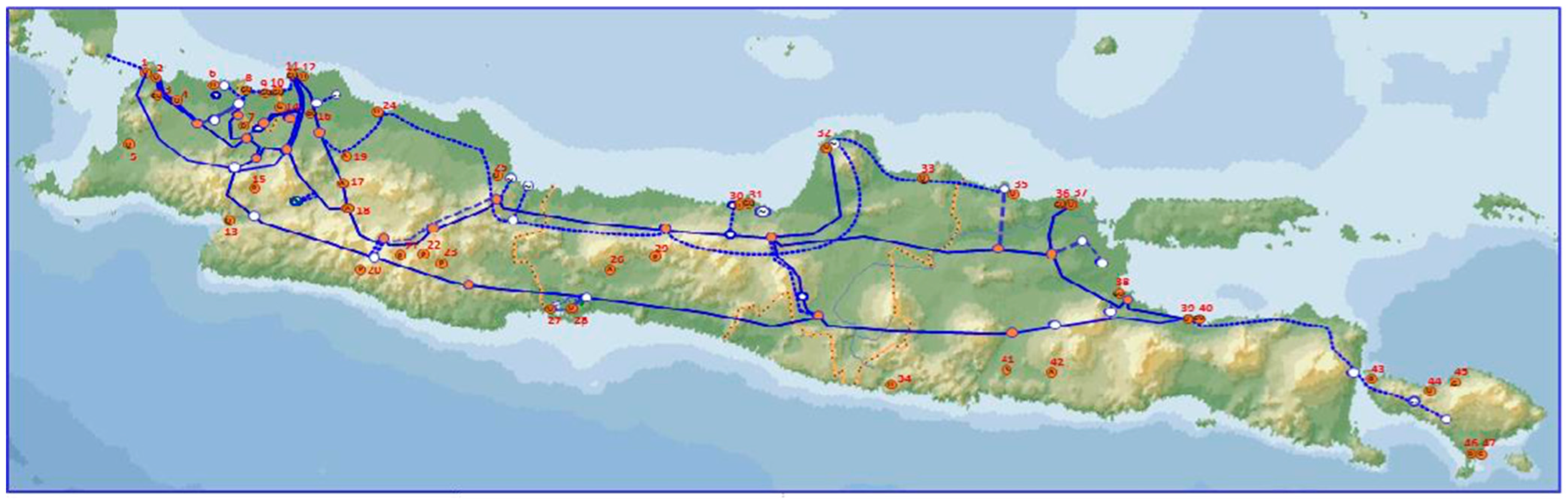
The Jawa Bali grid system, depicted in Figure 1, plays a vital role in providing power to the islands of Java and Bali in Indonesia, supporting their sizable populations and industrial sectors. With an installed capacity of 47,647 megawatts (MW) in 2023, it ranks among the most substantial electricity grids in Southeast Asia [1]. During that year, the system faced a peak load of approximately 40,223 MW during peak hours, indicating a relatively narrow margin between capacity and demand [1].

Figure 1.
The Jamali Power System. Reprinted from Ref [3].
As of 2022, the population of the combined regions of Java and Bali in Indonesia is estimated to be around 157 million [4]. The expected population growth for Jawa and Bali regions to 2029 is projected to be significant, driven by factors such as natural population increase (births exceeding deaths) and migration from other parts of Indonesia to these regions. While specific population projections can vary depending on various factors and assumptions, it is estimated that the population of Jawa and Bali regions could surpass 164 million by 2029 (around 0.8% growth [4]).
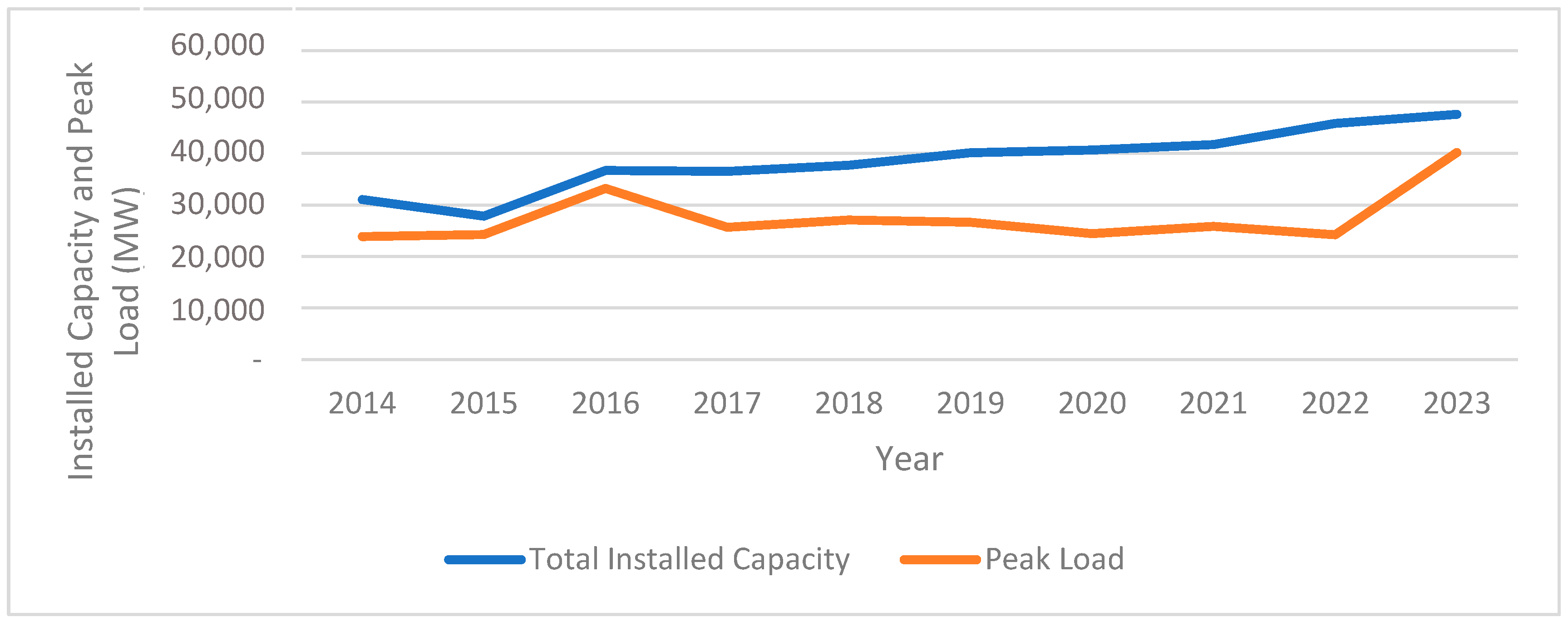
However, the region’s rapid economic expansion and urbanization are anticipated to drive an annual peak load increase of about 8%. To accommodate this growth and ensure a dependable power supply, significant investments are being made in infrastructure and renewable energy sources to bolster the Jawa Bali grid system. The average capacity growth, depicted in Figure 2, from 2014 to 2023 is 5.37%, according to PLN’s Statistic data from 2014 to 2023 [5] (pp. iii, 1–3).
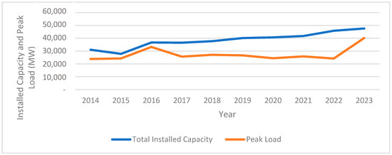
Figure 2.
Jamali System Capacity and Peak Load Demand for 2014–2023.
Two key variables of Jamali system important for this simulation are peak load and installed capacity. Peak load represents the highest load reached by each system within a calendar year. Installed capacity refers to the capacity of a single generating unit as indicated on the generator nameplate or prime mover, whichever is smaller [5]. Upon analyzing historical supply–demand data from the Jamali system, a notable increase in peak load is observed in 2023. This surge could suggest a rise in demand attributable to the growth of electric vehicles (EVs).
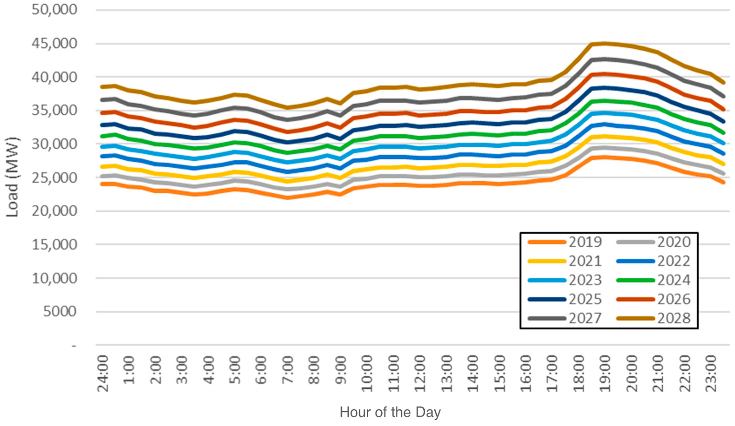
The peak load for the Jawa-Bali grid system, as illustrated in Figure 3, typically occurs between 18:00 and 19:00, when demand is at its highest. This peak load is influenced by several factors, including the time of day, season, and level of economic activity.
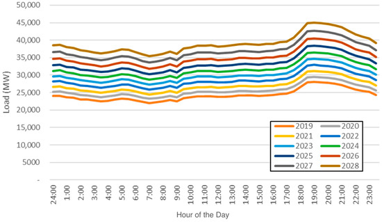
Figure 3.
Jamali Hourly Peak Load. Reprinted from Ref [6].
A crucial aspect of this simulation is the determination of the base peak load, which represents the electricity demand excluding the demand from electric vehicles (EVs). While obtaining this metric can be challenging, it can be estimated through extrapolation of historical data. Since the number of EVs before the introduction of subsidies and regulations in 2023 was minimal, their load demand was insignificant. Therefore, the peak load before that year can be closely regarded as the base peak load.
1.2. Java and Bali’s EV Growth
The electric vehicle (EV) market in Indonesia is poised for significant growth over the next five years, with a range of factors driving this expansion. The government’s supportive policies, including tax incentives and subsidies, are expected to encourage more consumers to switch to EVs [7]. Additionally, the country’s commitment to reducing carbon emissions and addressing air pollution is likely to drive the demand for cleaner transportation options.
In terms of EV preferences, the market in Indonesia is expected to be diverse. While there is a growing interest in luxury EVs, especially among affluent consumers in urban areas, there is also a significant demand for more affordable EVs that cater to daily commuting needs. In 2023, Hyundai sold 7176 units of the Ioniq 5 and Wuling sold 5575 units of the Air EV [8]. They have the highest sales number that year. This dual focus of market preferences is expected to shape the EV market in Indonesia, with manufacturers offering a range of EV models to meet different consumer needs.
Charging infrastructure is a crucial factor in the growth of the EV market and Indonesia is making efforts to expand its charging network. While slow-/home charging is more widely available and convenient for daily use, fast-/public charging stations are also being installed, particularly along major highways and in urban centers, to cater to longer trips and provide more flexibility to EV owners. As the charging infrastructure continues to improve, it is expected to further boost consumer confidence in EVs and drive their adoption in Indonesia. As the beginning of 2024, 1124 public charger were made available by PLN [9]. This does not count public charger made available by landowners or private companies.
1.3. Indonesia’s EV Regulations and Subsidies
Indonesia has been implementing several regulations and incentives to encourage the adoption of electric vehicles (EVs) and address environmental and energy challenges. Some of these regulations include:
- Odd–even license plate policy: In major cities like Jakarta, the odd–even license plate policy restricts vehicles based on their license plate numbers on certain days. This measure aims to reduce traffic congestion and air pollution, indirectly encouraging the use of EVs [10].
- Tax reduction: The government offers tax incentives for EVs, including lower import duties and luxury goods tax exemptions. These incentives make EVs more affordable for consumers and help stimulate the EV market [11].
- Parking benefits: Some cities provide free or discounted parking for EVs to incentivize their use. This can reduce the overall cost of owning an EV and make them more attractive to consumers [12].
- Charging infrastructure: The government has been investing in EV charging infrastructure to support the growth of the EV market. This includes installing charging stations in public areas and along highways [9].
In terms of subsidies, the Indonesian government has implemented additional programs to expedite this transition. These include a 10% VAT tax deduction for four-wheeler electric vehicles (4wEV), as outlined in Ministry of Finance Regulation number 38 of 2023 [13], and an IDR 7,000,000 deduction for two-wheeler electric vehicles (2wEV), as specified in Ministry of Industry Regulation number 6 of 2023 [14].
The political landscape in Indonesia plays a crucial role in influencing the growth of electric vehicles (EVs) in the country. The regulations and subsidies pertaining to EVs until 2029 will be determined by the President elected in 2024, who will serve a single term of five years [15].
1.4. Literature Review and Contribution Overview
To contextualize this study, related works on EV integration into power grids and their impact on supply–demand balance are reviewed. Previous research has highlighted the challenges of integrating EVs into existing grids, emphasizing the need for advanced simulation models to predict and manage these impacts. However, there remains a gap in incorporating dynamic factors such as population growth and peak load variations, which this study aims to address.
Previous research papers have explored simulations to forecast EV load AI-based demand load prediction utilizing historical data by utilizing artificial neural network (ANN) and recurrent neural network (RNN) methodologies for predicting demand for plug-in hybrid electric vehicles (PHEVs) [16], as well as factors like temperature and traffic that are often overlooked in conventional EV load prediction models [17] and user behavior data [18]. Additionally, a simulation has been developed by considering variables such as the state of charge, arrival time, charging duration, charging rate, maximum charging power, and engagement rate [19].
Others have explored various impacts of electric vehicle (EV) growth and proposed solutions. These include the use of Vehicle-to-Grid (V2G) technology, which enables EV load to serve as distributed energy resources that contribute to grid stability. V2G systems operate by charging EVs during periods of low electricity demand, typically off-peak hours, and discharging them back to the grid during peak demand, thereby mitigating fluctuations and enhancing grid stability [20]. Another solution is a coordinated charging to manage load demand surges by utilizing pricing mechanisms to guide EV charging, which has emerged as a significant policy tool for demand-side management [21].
This paper is novel in its approach as it introduces a dynamic simulation model that overcomes the limitations of existing static growth simulations identified in the literature. By integrating multiple growth factors and enabling real-time adjustments, this study offers a more comprehensive and precise representation of the interactions between electric vehicle (EV) adoption and grid dynamics. These contributions effectively address critical research gaps and provide valuable insights for policymakers and grid managers. The primary contributions of this paper are as follows:
- Novel Simulation Approach: Introduces a novel approach to simulating the impact of EVs on the grid’s supply–demand balance, with a specific focus on the regions of Jawa and Bali.
- Policy and Subsidy Management Tool: Provides a tool to predict optimal management strategies for the increasing number of EVs, considering the effects of policies and subsidies.
- Dynamic Simulation Model: Shifts from traditional static growth simulations to a dynamic simulation model implemented in MATLAB R2021b and Simulink 10.4.
- Comprehensive Growth Factor Integration: Incorporates seven key yearly growth factors:
- ₋
- Power plant capacity
- ₋
- Base peak load demand
- ₋
- Personal vehicle growth
- ₋
- EV attractiveness
- ₋
- Subsidy impact
- ₋
- Vehicle type
- ₋
- Charging preferences
- Accurate Grid Dynamics Representation: Delivers a more accurate representation of the complex interactions between EV adoption and grid dynamics, effectively filling gaps in the existing literature.
- Valuable Tool for Policymakers: Offers policymakers a robust simulation tool for managing the integration of EVs into the grid more effectively.
- Flexible Scenario Modeling: Allows for the adjustment of simulation inputs to model specific scenarios, enhancing the flexibility and applicability of the simulation.
- Potential for Further Development: Demonstrates potential for further development to include additional growth factors, thereby increasing the accuracy and realism of the simulation outputs.
2. Data Gathering and Data Analysis
The analysis initiates with the acquisition of data pertaining to the present and anticipated growth of variables impacting both the supply and demand aspects of the grid. These data are imperative for the execution of the simulation.
2.1. Power Grid Capacity
Most of the data regarding the current supply and base demand of the grid, along with its historical data and predicted growth factors, are sourced from the annual reports of Indonesia’s sole national electricity company (PLN), referred to as RUPTL. Statistic reports from RUPTL and PLN from 2014 to 2023 have been considered to enhance the accuracy of historical data and growth projections. This historical data are presented in Table 1.

Table 1.
Jamali System Supply and Demand Historical Data. Reprinted from Ref [1,5].
Utilizing the National Electricity Company’s data (RUPTL) [3], an analysis of the Jamali electricity supply can be conducted. The supply side of the grid is simulated by projecting the current capacity, depicted in Table 2, and a growth factor based on the RUPTL.
Table 2.
Supply Side Input Variables Values.
2.2. Demand Peak Load
The demand side of the grid contains two main components, including the base peak load that excludes the electric vehicle load and the EV load itself. A demand simulation model for the EV load was created to calculate the total increase in demand load with a combination of ICE and the electric vehicle population, initial charging time (ICT), the ratio between slow and fast charging, and the charge load curve of each type of vehicle using the data gathered. The variables related to the demand side and their values, as presented in Table 3, are as follows:
Table 3.
Demand side input variables values.
- Base Peak Load (excluding EV Load Demand) [1,5]
- Jamali Population [4]
- Personal Vehicle Population [22]
- Electric Vehicle Population Probability [23]
- The Ratio of 2- to 4-Wheeled EVs [22]
2.3. Initial Charging Time
In the simulation of demand load, it is imperative to account for the initial charging time (ICT), denoting the moment when EVs are connected to the grid for daily charging. For most EV users, ICT can be approximated as coinciding with the conclusion of their daily travel, as illustrated in Figure 4. As per the National Household Travel Survey (NHTS) findings, the distribution of end-of-travel times depicted in the graph conforms to a normal distribution [24]. Subsequently, the data for hourly initial charging times is segmented into intervals of 12 min each (5 ICTs per hour, with a resolution of 12 min), depicted in Figure 5. The probability density function of the graph is presented below.
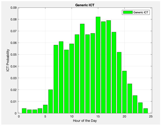
Figure 4.
Generic Initial Charging Time.
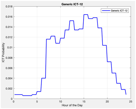
Figure 5.
ICT with 12-Minute Resolution.
2.4. Electric Vehicle’s Specification Details and Charge Curve
The total load demand will be divided into two categories: two types of four-wheeled EVs (4wEV) and two types of two-wheeled EVs (2wEV). Each category represents both a luxury and a daily-use type of vehicle for both four-wheeled and two-wheeled EVs. The samples are as follows:
- 2021 Hyundai Ioniq 5 Long Range
- 2023 Wuling Air EV Long Range
- 2022 United TX1800
- 2023 Viar new Q1L, with following specifications detailed in Table 4:
Table 4. EV Type Specifications.
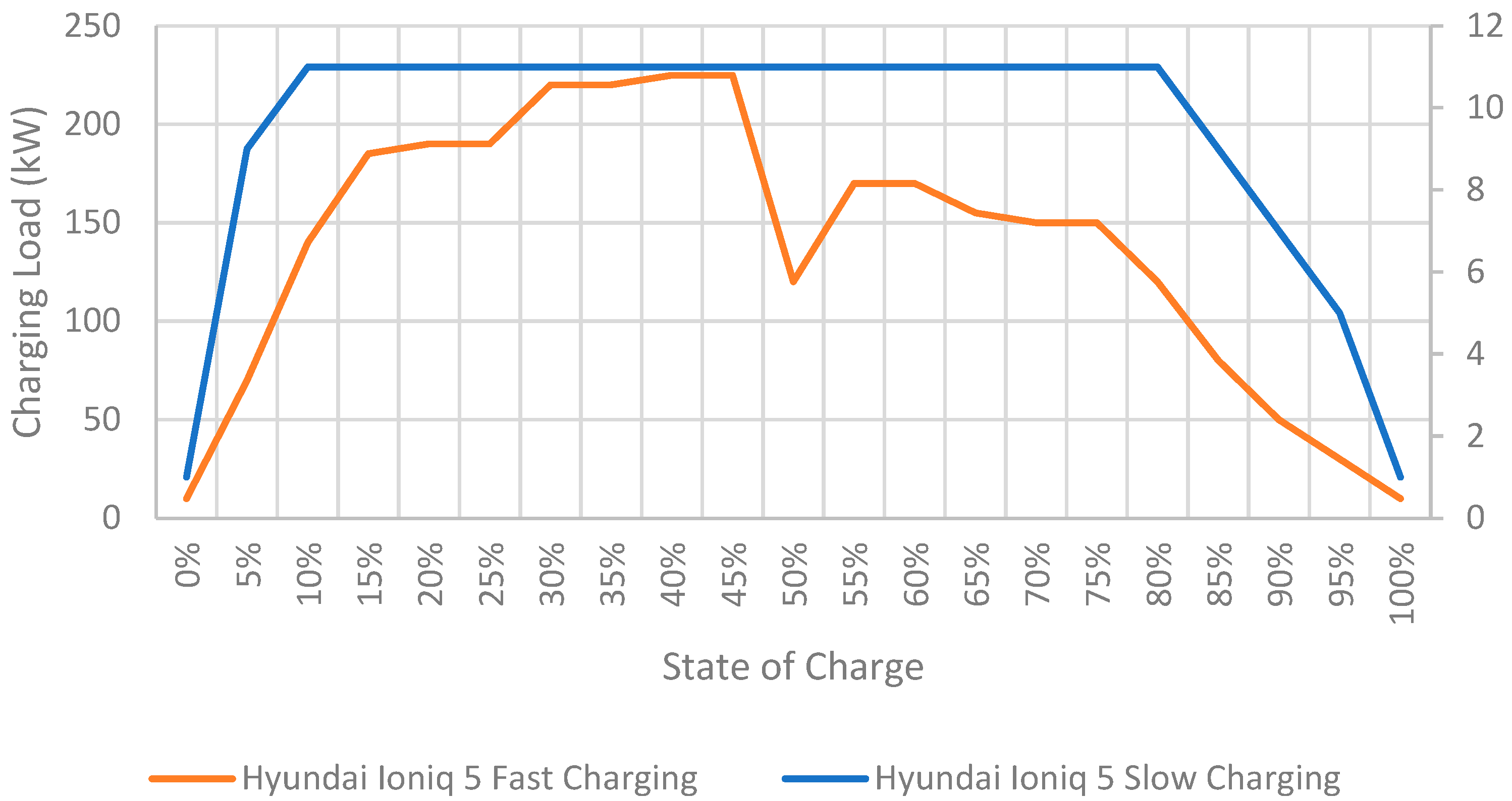
The charging load data for four-wheeled electric vehicles (4wEV) is based on the charge load curve of the 2021 Hyundai Ioniq5, which features a 72.6 kWh battery capacity [25]. The Hyundai Ioniq is Indonesia’s top-selling 4wEV, with 7.176 units sold in 2023 [8]. During slow charging mode, the peak load of the Ioniq5 is 7.2 kW, while the peak demand during fast charging mode reaches 225 kW [25].
The frequency of charging for an electric vehicle (EV) is determined by the total travel distance covered per charge. For example, the IONIQ 5, with a range of 450 km [25], divided by a norm of 30 km traveled each day [26], would require charging approximately every 15 days. Figure 6 illustrates the charge curve of the IONIQ, as measured during charging [27].
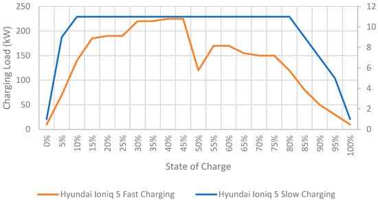
Figure 6.
Hyundai Ioniq 5 Long Range Charge Curve.
Another source for charging load data for budget four-wheeled electric vehicles (4wEV) was obtained from the Wuling Air EV Long Range model [28]. The Air EV is the second best-selling 4wEV unit in 2023 [8]. Unlike the Ioniq5, it does not feature fast charging capability. Based on the average daily commute, the Wuling Air EV Long Range model requires charging approximately every 10 days. Figure 7 illustrates the charge curve of the Wuling Air EV.
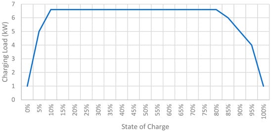
Figure 7.
Wuling Air EV Long Range Charge Curve.
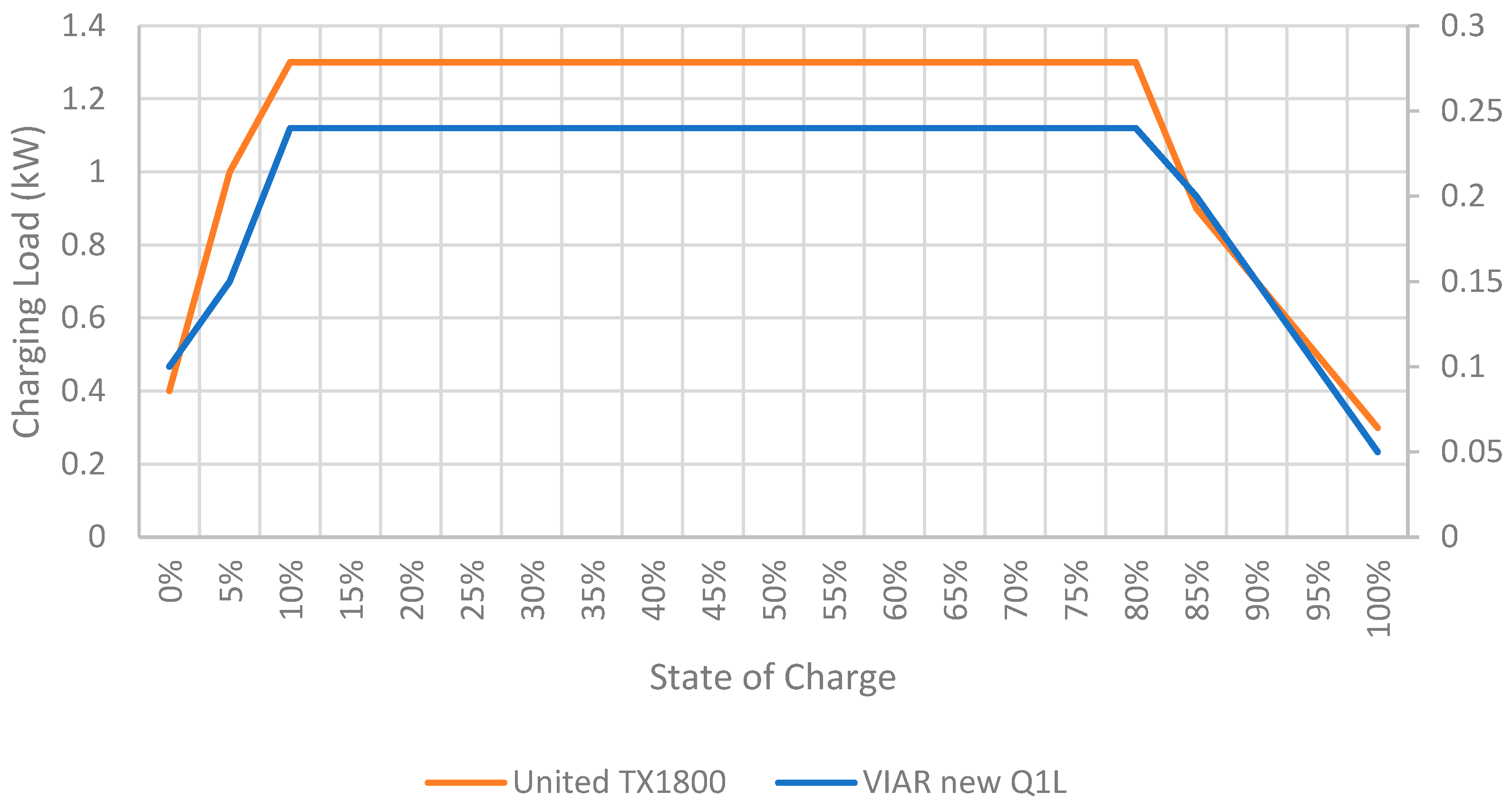
The total load from two-wheeled electric vehicles (2wEV) is calculated using charge load data obtained from the United TX1800 [29] and the budget-oriented VIAR new Q1L electric motorcycle, which was a pioneer of 2wEV in Indonesia in 2017 [30]. The United TX1800 has a 1300 W charge peak [29], while the VIAR new Q1L has a 0.24 kW peak [30]. The daily distance traveled and initial charging time (ICT) are similar to the 4wEV load simulation. Generally, 2wEVs in Indonesia do not feature fast charging capabilities. Figure 8 illustrates their charge curves.
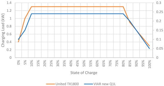
Figure 8.
United TX 1800 and VIAR New Q1L Charge Curve.
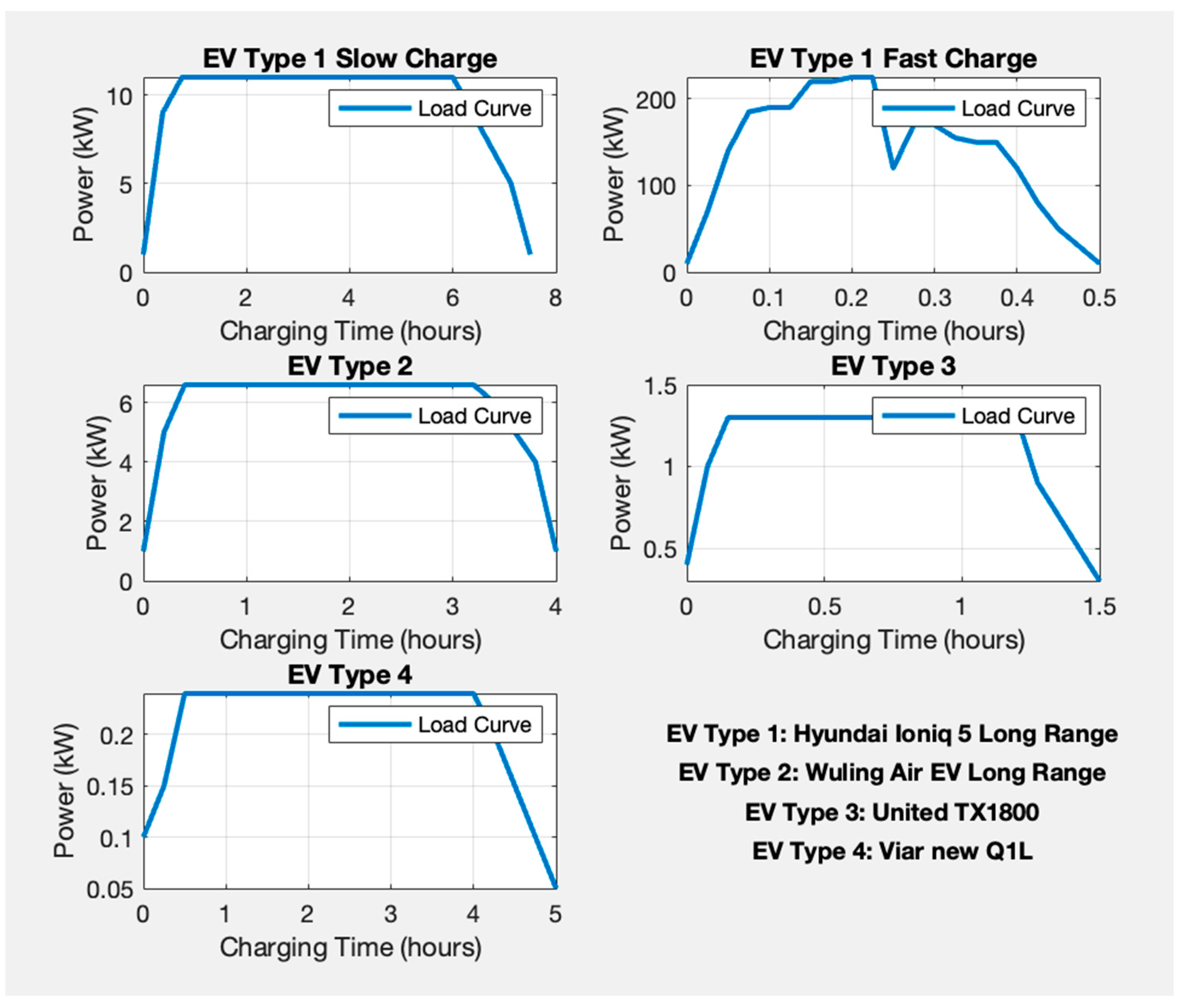
These charge curves, depicted in Figure 9, are utilized as inputs in the demand simulation. The total additional electricity demand from EVs is determined by the combination of the number and type of vehicles, ICT, and the fast/slow charging curve of each vehicle. The charge curves from each EV type used in the simulation are shown below.
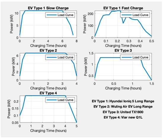
Figure 9.
EV Charge Curves.
3. Simulations
The simulation model was developed using MATLAB and Simulink. MATLAB was chosen for this supply–demand simulation due to its powerful computational capabilities, which can efficiently handle complex models and large datasets. Its integration with Simulink provides a graphical environment for modeling and simulating dynamic systems, essential for power grid analysis. MATLAB’s flexibility allows for custom scripts and functions to tailor simulations to specific needs. It excels in data handling and visualization, aiding in the interpretation of results. Additionally, MATLAB’s interoperability with other software and languages supports a multidisciplinary approach, and its optimization for modern hardware ensures faster simulations and the efficient handling of complex models. These features collectively make MATLAB an effective choice for accurate supply–demand simulations in power grid and EV integration contexts.
For running these simulations, a high-performance PC is typically required. This usually includes a multi-core processor (such as an Intel i7 or better), at least 16 GB of RAM (32 GB or more is recommended for large-scale simulations), and a solid-state drive (SSD) for faster data access and storage. In this study, the simulations were performed on an Apple M1 chip with 8 GB of RAM. Despite the relatively modest hardware, the total simulation time was less than 1 h, demonstrating the efficiency of the simulation setup and the capabilities of the chosen hardware. This efficiency ensures that multiple scenarios can be tested and analyzed within a reasonable timeframe.
Key components of the model and their interactions in this simulation, as illustrated in Figure 10, are outlined below:
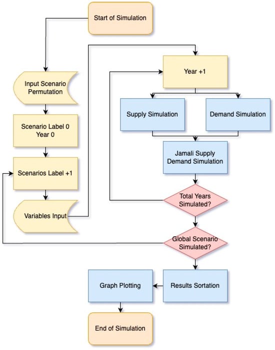
Figure 10.
Flowchart of the Simulation.
- Scenario Permutations: The simulation begins with the permutation of input scenarios. Each permutation provides values for the variables. With 3 possibilities for each of the 7 different variables, this results in 2187 scenarios.
- Supply–Demand Simulations: Based on the values of each scenario, the supply and demand simulations commence. Each supply–demand simulation runs for five years, covering the period from 2024 to 2029.
- Simulink EV Load Simulation Models: Charge load simulations are conducted individually for each type of EV.
- Output Assessment and Sortation: Scenario outputs are sorted based on their EV percentage by 2029, cost allocation for the additional yearly electricity supply, and cost allocation for the yearly EV subsidies.
3.1. Variable Inputs
The simulation incorporates two primary groups of inputs, each processed at different stages of the simulation. Initially, global input parameters are processed at the beginning of the simulation during the scenario development and permutation phase. Subsequently, the supply–demand simulation utilizes variable inputs, which are dynamic and updated annually based on the scenario effects and the previous year’s simulation outcomes.
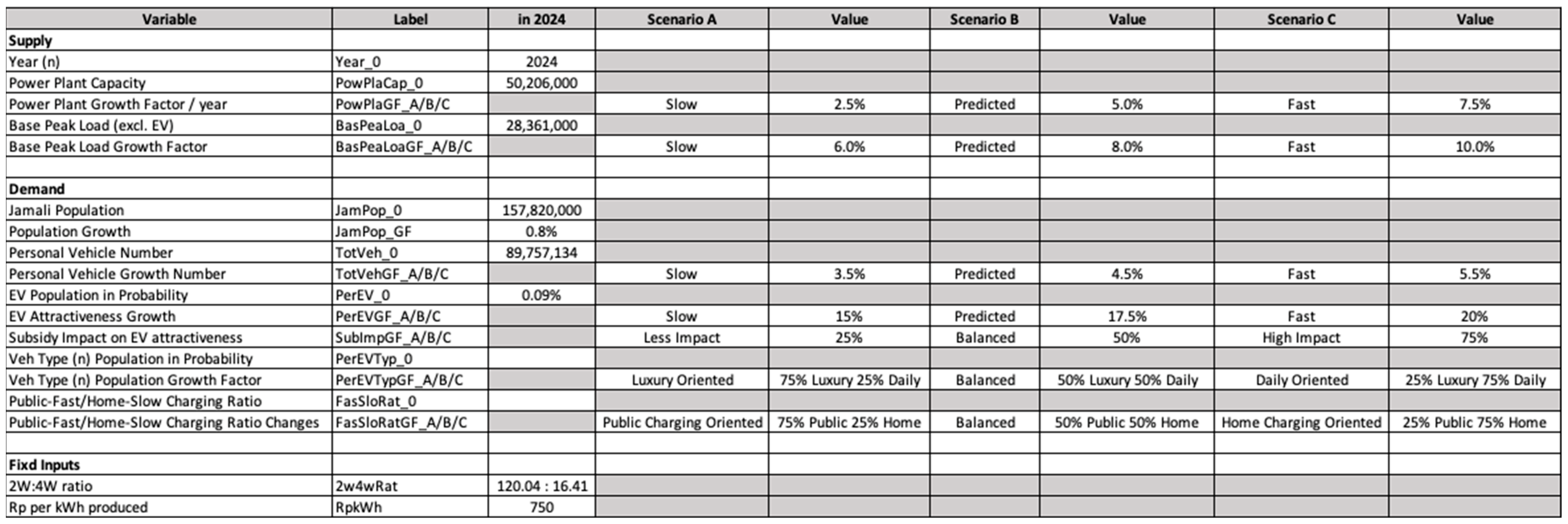
The global variable inputs, presented in Table 5, establish the scenario and growth factors that influence the trajectory of the simulation. These inputs depict the impacts of policies, market conditions, subsidy effects, and public preferences over a five-year period. The global variable inputs include the following:
Table 5.
Global Variable Inputs.
The variable inputs for the supply–demand simulation, however, will specifically affect the outcomes of each annual supply–demand simulation. The results from the previous year’s simulation will serve as inputs for the subsequent year. Table 6 presents the variable inputs for the supply–demand simulation:
Table 6.
Supply–Demand Variable Inputs.
Within the demand simulation, there are inputs specific to each type of EV. These variable inputs include the following:
- EV Type Population
- Driving Range
- Battery Size
- DC Fast Charging Capability
- Charging Duration
- Maximum Charging Load
- Yearly Sales
- Production Start
For simulation time efficiency, certain input factors have been excluded from the current model. These factors will be incorporated in the next development phase of the simulation to enhance its accuracy and comprehensiveness. Specifically, the negative growth of EV attractiveness, which accounts for potential declines in EV adoption based on market conditions and consumer preferences identified in the literature review, has been omitted. Additionally, the simulation does not currently consider negative growth in base load, which reflects scenarios where the overall electricity demand decreases due to factors such as increased energy efficiency or economic downturns. The detailed input factors are attached in Appendix A.
Lastly, the current simulation does not include the regulatory effect of load, where an increase in load causes a voltage drop and consequently a decrease in load. However, this omission does not significantly impact the simulation’s outcomes because the model focuses on the maximum peak load for each scenario. By considering the maximum peak load, the simulation captures the critical stress points on the grid, which are the primary concern for grid stability and planning. Therefore, while the regulatory effect of load is an important aspect, its exclusion in this context does not undermine the overall reliability and relevance of the simulation results.
3.2. Scenario Development and Permutations
In addition to the supply–demand simulations for the period 2024–2029, various scenarios are to be simulated. Each scenario involves variations in the growth speed of each supply–demand simulation’s input variable. These variations in growth factors include the following:
- Power Plant Capacity Growth [1,5]
- Base Peak Load Growth Factor, using historical data projection [1,5]
- Personal Vehicle Growth Factor [2,31]
- Electric Vehicle Attractiveness Growth Factor [32]
- Subsidy Impact on EV Attractiveness
- Vehicle Type Preferences
- Home/Public Charging Preferences, with the following values
The seven growth factors, as presented in Table 7, substantially influence the grid’s supply–demand balance. The first two factors, power plant capacity and base peak load growth, determine the remaining available capacity that can be allocated for EV charging load.
Table 7.
Input Variation’s Value.
The subsequent three factors, including personal vehicle growth, EV attractiveness, and the impact of subsidies on EV attractiveness, will determine the total number of EVs in each given year.
The final two factors, namely, vehicle type and preferences for home or public charging, will define the specific charging load curve for each simulated EV.
These factors collectively encompass most of the variables necessary to determine the grid’s supply–demand balance. Based on the annual outputs of these scenarios, the simulation will assess the impact on EV growth, cost allocation for supply adjustments, and cost allocation for EV subsidies, which are the primary outputs to be evaluated when analyzing each scenario.
For each growth factor, three scenarios—A, B, and C—are provided. For power plant capacity, base peak load demand, personal vehicle growth, and EV attractiveness growth factors, scenario B simulates the predicted growth factor based on the literature. Scenarios A and C simulate slower and faster growth factors, respectively, according to the literature and historical data.
The subsidy impact growth factor in scenario B reflects a balanced 50% impact based on the literature research, while scenarios A and C depict a lesser 25% impact and a higher 75% impact, respectively. Vehicle type and home/public charging preferences are given a balanced 50:50 ratio for scenario B, with a 75% preference for each charging type in scenarios A and C.
In combinatorial mathematics, a permutation refers to the different ways of selecting and arranging objects. It represents an arrangement of objects in a specific order. When repetition is allowed and the order matters, the number of possible permutations of r elements taken from a set of n elements is given by (nr) [33].
nr = 37 = 2187
Since the repetition of combinations is allowed, each of the 7 variable inputs can be filled with any of the 3 growth factor speed variations, giving us 2187 possible scenarios.
3.3. Power Plant Capacity and Base Load Profile Simulation
The collected data will serve as inputs in MATLAB and will be simulated in Simulink. The power plant capacity will act as the supply capacity in the simulation. The current capacity and its projected growth factor were sourced from the RUPTL PLN. The projection is using the formula for compound growth.
where:
Vn = V0 × (1 + GF)t
- Vn is the variable’s value at year n.
- V0 is the initial value at year 0.
- GF is the growth factor based on the scenario simulated.
- t is the number of years between year n and year 0.
Actual Power Plant Capacity = Capacity in 2024 × (1 + Capacity Growth Factor) ^ Number of Year
The base peak load, which excludes EV load, is also simulated using its current value and growth factor.
Actual Base Peak Load = Base Load in 2024 × (1 + Base Load Growth Factor) ^ Number of Year
3.4. EV Load Simulation
The EV demand load was calculated based on the Jamali population and its ratio to vehicle ownership. A certain percentage of these vehicles are EVs. The growth factor of EVs is influenced by their attractiveness and the impact of EV subsidies.
Actual Jawa Bali Population = Population in 2024 × (1 + Population Growth Factor) ^ Number of Year
Equation (5) calculates the actual population of Jawa Bali in any given year based on the population in 2024 and an annual population growth factor. This equation accounts for the number of years since 2024 and multiplies this by the growth factor and the initial population, providing an estimate of the population growth over time. This is crucial for understanding the demographic changes that influence transportation needs and energy consumption.
Actual Total Vehicle Population = (Actual Jawa Bali Population × Vehicle to Population Ratio) + (Number of Year × Vehicle Growth Factor × Total Vehicle Population in 2024)
Equation (6) determines the actual total vehicle population by considering both the current population of Jawa Bali and the annual vehicle growth factor.
EV Growth Factor = EV Attractiveness Growth Factor + Subsidy Impact Growth Factor
Equation (7) calculates the EV growth factor by summing the EV attractiveness growth factor and the subsidy impact growth factor. This reflects the combined effect of market attractiveness and governmental incentives on EV adoption.
Actual EV Population = Total Vehicle Population × Total Vehicle to EV Ratio + (Number of Year × EV Population Growth Factor + EV Population in 2024
Equation (8) estimates the actual EV population by considering the total vehicle population, the ratio of total vehicles to EVs, and the annual growth factor of EVs, adjusted by the number of years and the initial EV population in 2024.
The demand simulation then progresses in Simulink. The simulations are conducted individually for each type of EV: including EVTyp_1F, EVTyp_1S, EVTyp2, EVTyp3, and EVTyp4.
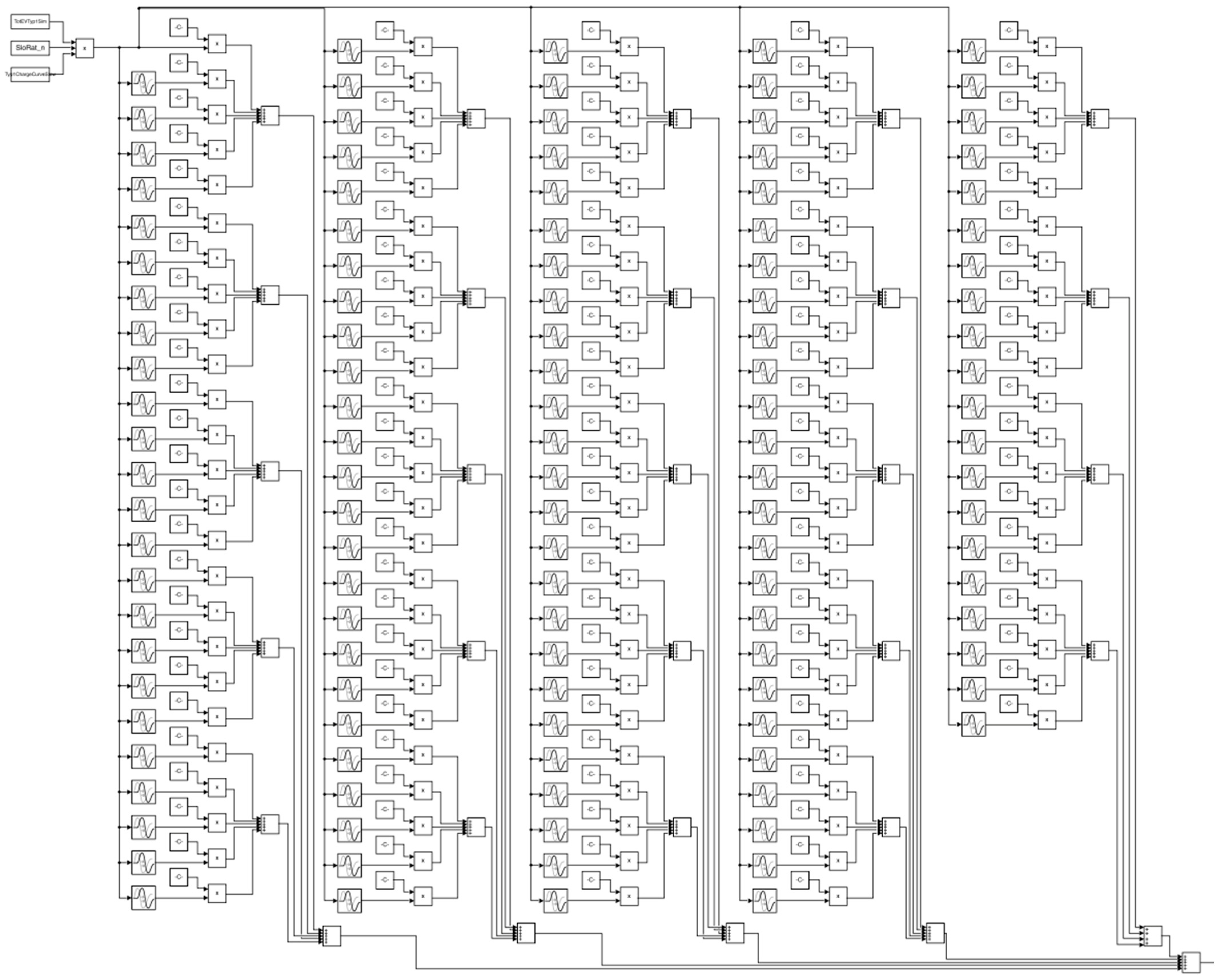
A novel Simulink model, as presented in Figure 11, was developed to simulate the demand dynamics of each EV types charging loads. The model’s primary inputs for each simulation include the number of vehicles for each given year and scenario, the ratio of home and public charging, and a charge load curve specific to each charging process. The vehicle count for each EV type is simulated by extrapolating the current number of vehicles using a growth factor specific to each scenario.
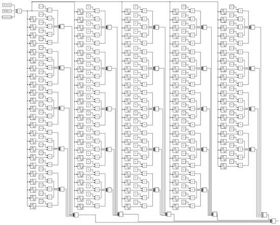
Figure 11.
Simulink Model of Load Demand Simulation for Each EV Type.
These inputs, in conjunction with the ICT, determine the number of charging processes initiated at each time of the day. If a previous charging process overlaps with another during the subsequent ICT, the loads are aggregated to simulate the cumulative charging load at each time interval. The total load is then modeled over a 24-h period with a resolution of 12 min.
3.5. Simulation’s Output Assestment and Sortation
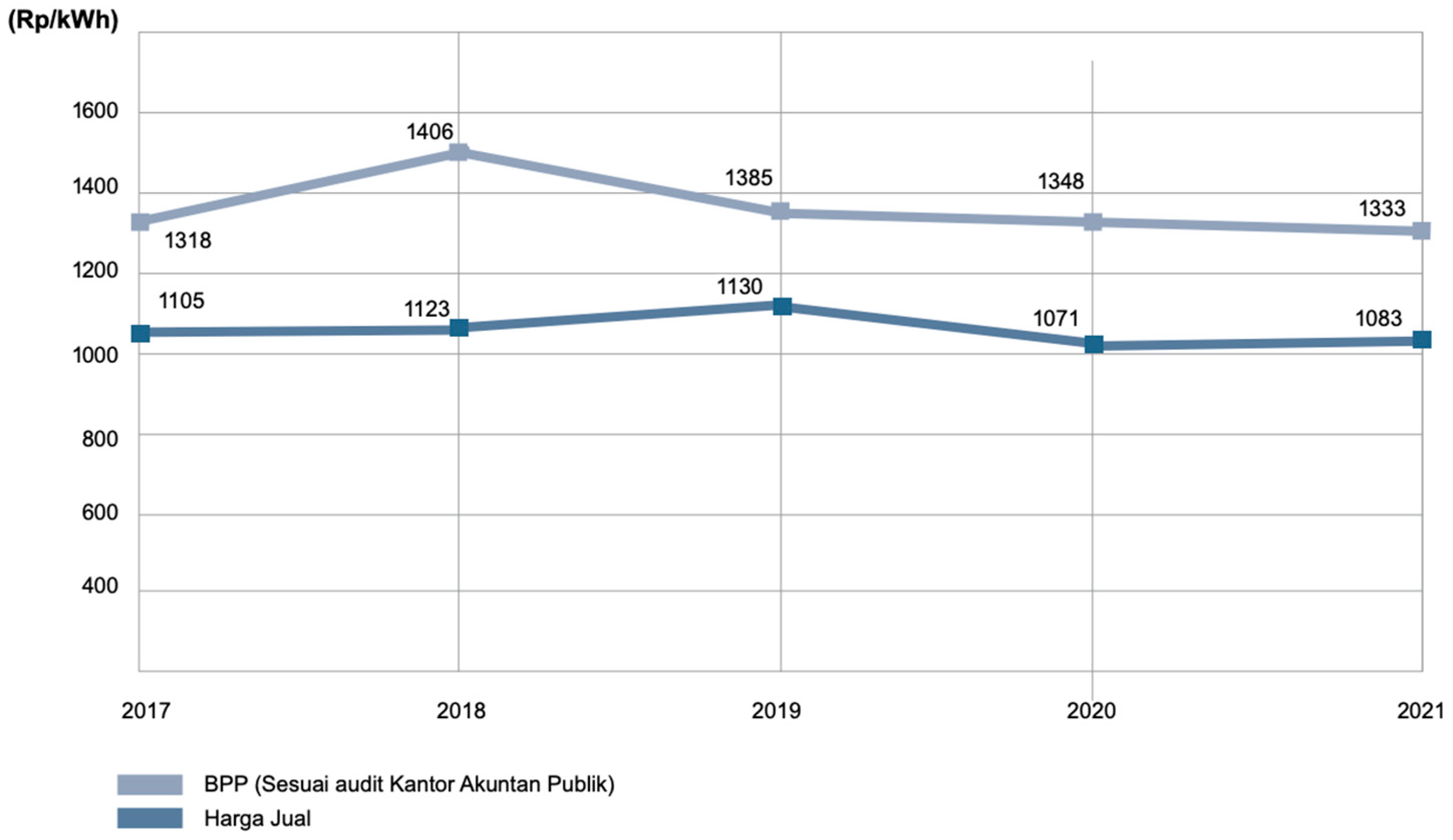
The three main outputs for each scenario are the end EV percentage by 2029, cost allocation for the additional yearly electricity supply, and cost allocation for the yearly EV subsidies. The total cost allocation for the additional yearly electricity supply was simulated by considering the deficit in power plant capacity by the end of 2029. The average supply cost per kilowatt-hour (kWh) of Rp1108/kWh, as presented in Figure 12, was derived from BPP PLN [34].
Cost Allocation for Additional Electricity Supply = (Total Simulated Load 2029 − Power Plant Capacity 2029) × Supply Cost
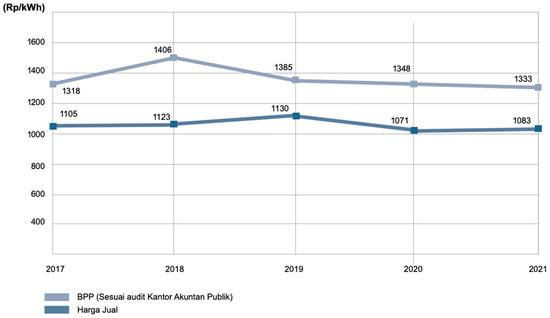
Figure 12.
Supply Cost per kWh (BPP PLN) for 2018–2022. Reprinted from Ref [34].
On the contrary, the cost allocation for the yearly EV subsidies was determined by considering the surplus of the power plant capacity. To achieve a balance in the grid’s supply and demand, a specific number of EVs must be added to offset the supply. These include a 10% VAT tax deduction each 4wEV [13] and an IDR 7,000,000 deduction for each 2wEV [14].
Cost Allocation for the EV Subsidies = −(Total Simulated Load 2029 − Power Plant Capacity 2029) × Subsidy Cost
The outputs from each of the 2187 scenarios are sorted based on three criteria, as presented in Table 8. Given that EV growth is the primary goal of the government, the initial sorting criterion for the best scenarios is the highest EV percentage result in 2029. Subsequently, the scenarios are sorted by the minimum yearly cost allocation. Conversely, to identify the worst possible scenario, the simulation sorts by the least EV percentage with the highest yearly cost allocation.
Table 8.
Output’s Priority Order.
The second sortation criterion (cost allocation for the additional yearly electricity supply and cost allocation for the yearly EV subsidies) will offset each other depending on the power plant capacity deficit by the year 2029. Apart from presenting the best and worst possible outputs given the scenarios available, the simulation should be able to execute the inputted scenarios.
4. Results
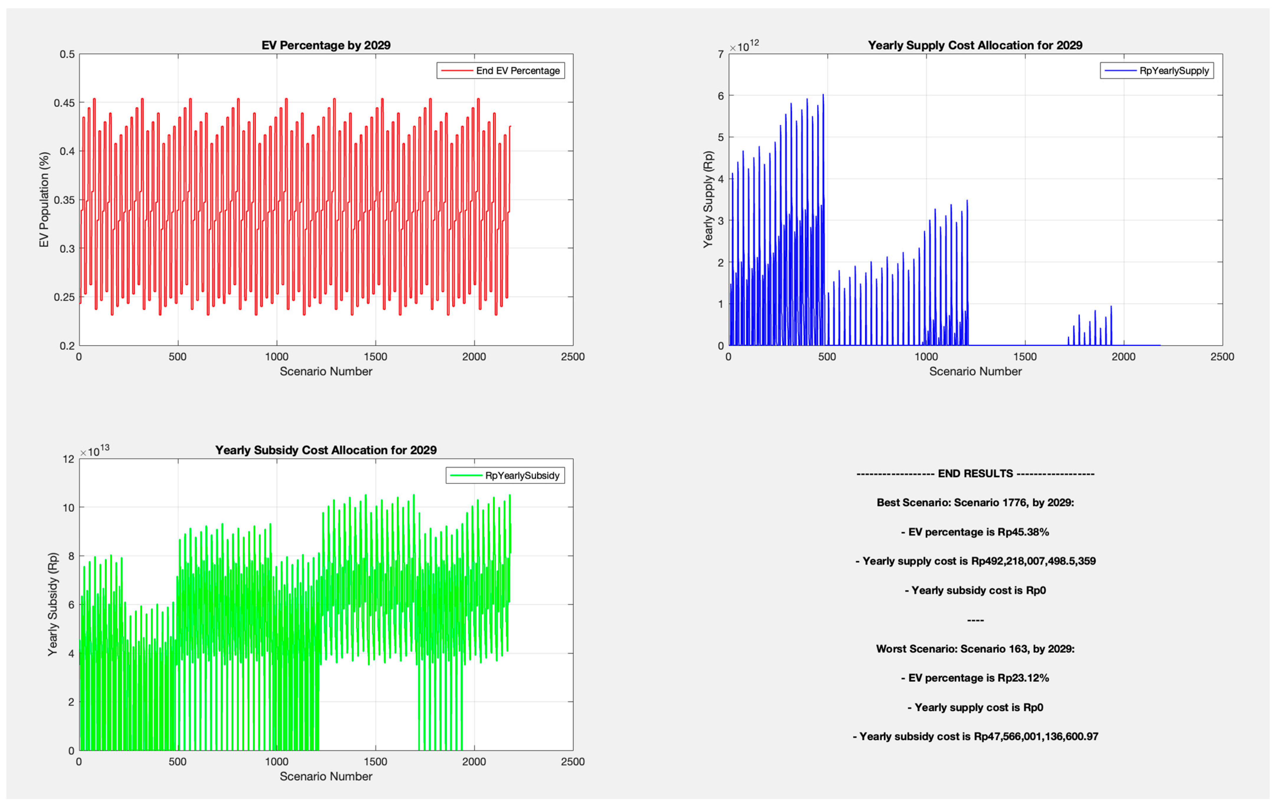
After simulating the 2187 scenarios, four results are worth considering: the scenario with the best outputs, the scenario with the worst outputs, and the most and least probable scenarios based on the information and predictions formed during the literature review. These four results should illustrate the magnitude of the impact that each input scenario has on the percentage of electric vehicles and the associated cost allocations. The detailed outputs are attached in Appendix B.
The scenario with the best result yielded the highest EV percentage of 45.38% by 2029 with the lowest yearly cost allocation for supply adjustment at Rp492,218,007,498. Conversely, the scenario with the worst result produced the lowest EV percentage of 23.12% by 2029 and the highest yearly cost allocation for subsidies at Rp47,556,001,136,600.
The most probable scenario resulted in an EV percentage of 42.98% and an annual subsidy cost allocation of Rp970,330,692,972. On the other hand, the least probable scenario yielded an EV percentage of 24.32% with an annual subsidy cost allocation of Rp45,475,187,899,827. The specifics of these four scenarios, as presented in Table 9, will be elaborated upon in the following sections.
Table 9.
Scenario Outputs.
4.1. Best Case Scenario
Based on the output simulation of 2187 scenarios for 2024–2029, the best-case scenario achieves the highest EV growth without disturbing the grid’s supply and demand balance. In the global scenario, all results were sorted, and the scenario with the highest EV percentage by 2029 was selected. Subsequently, all scenarios with the best EV percentage were sorted based on the lowest cost allocation for supply adjustment or subsidy allocation. The best-case scenario was labelled 1776. The input for this scenario permutation was 3213313, which translates to the following variable inputs (highlighted blue in Table 10):
Table 10.
Best Scenario Inputs.
This input scenario demonstrates that a rapid capacity expansion, coupled with a gradual and regulated increase in EV adoption, along with significant subsidies and a preference for home charging, can effectively balance the grid’s supply and demand. The best-case scenario resulted in the supply and demand details outlined in Table 11:
Table 11.
Best Scenario Outputs.
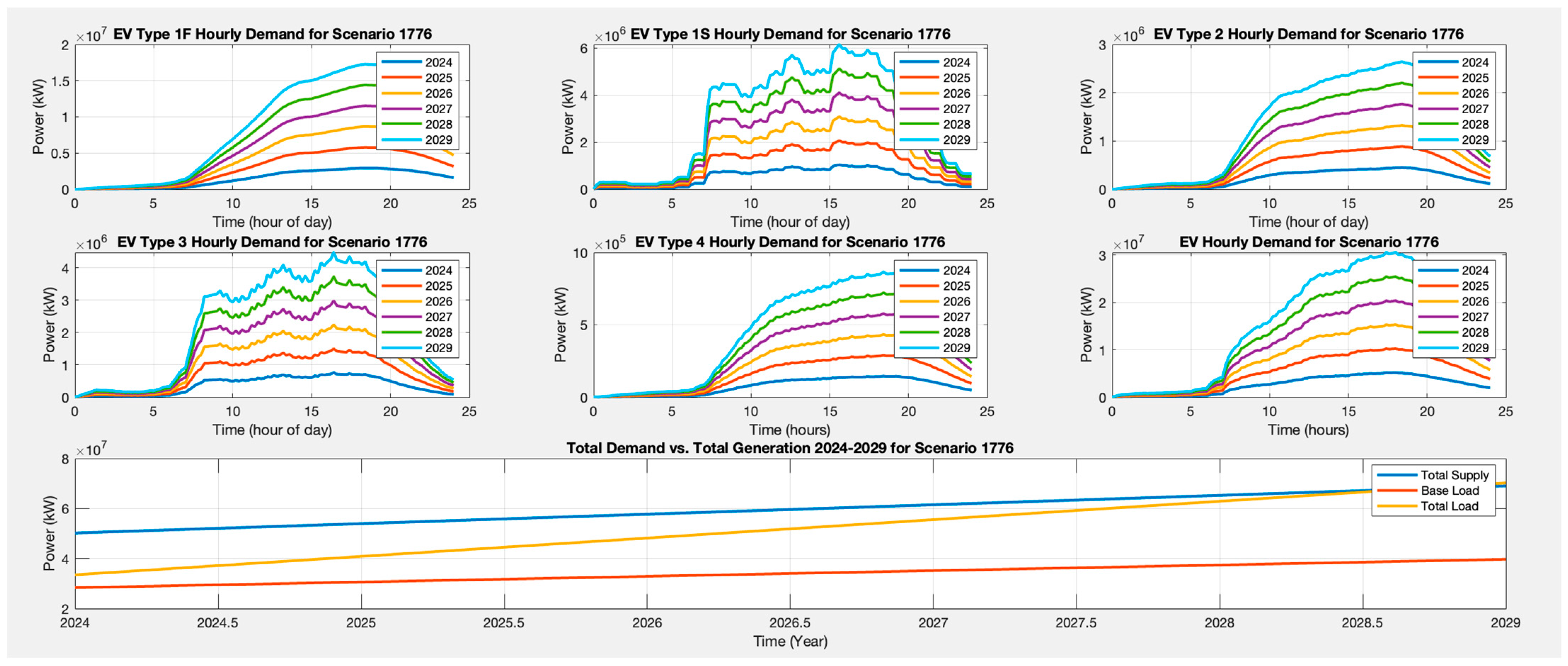
This input scenario resulted in the minimal disparity between the grid’s supply and demand, indicating a synchronized growth between the supply and demand sides of the grid. This scenario yielded the highest percentage of EV adoption with the lowest annual cost allocation. The hourly demand for each EV type and the total power plant deficit are displayed in Figure 13.
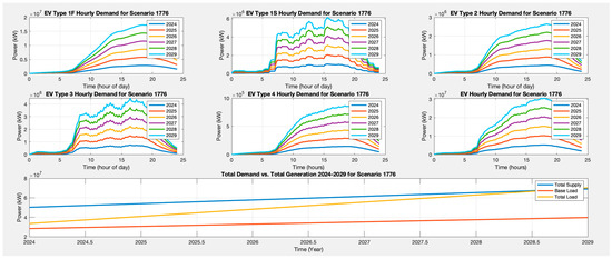
Figure 13.
Best Scenario Output Graphs.
4.2. Worst-Case Scenario
Based on the output simulation of 2187 scenarios for 2024–2029, the worst-case scenario was selected by sorting the scenarios with the least EV percentage in 2029. These scenarios were then resorted based on the highest cost allocation for supply adjustment or subsidy allocation. The worst-performing scenario was labeled 163. Its scenario permutation was 1131111 with the following input details (highlighted blue in Table 12).
Table 12.
Worst Scenario Inputs.
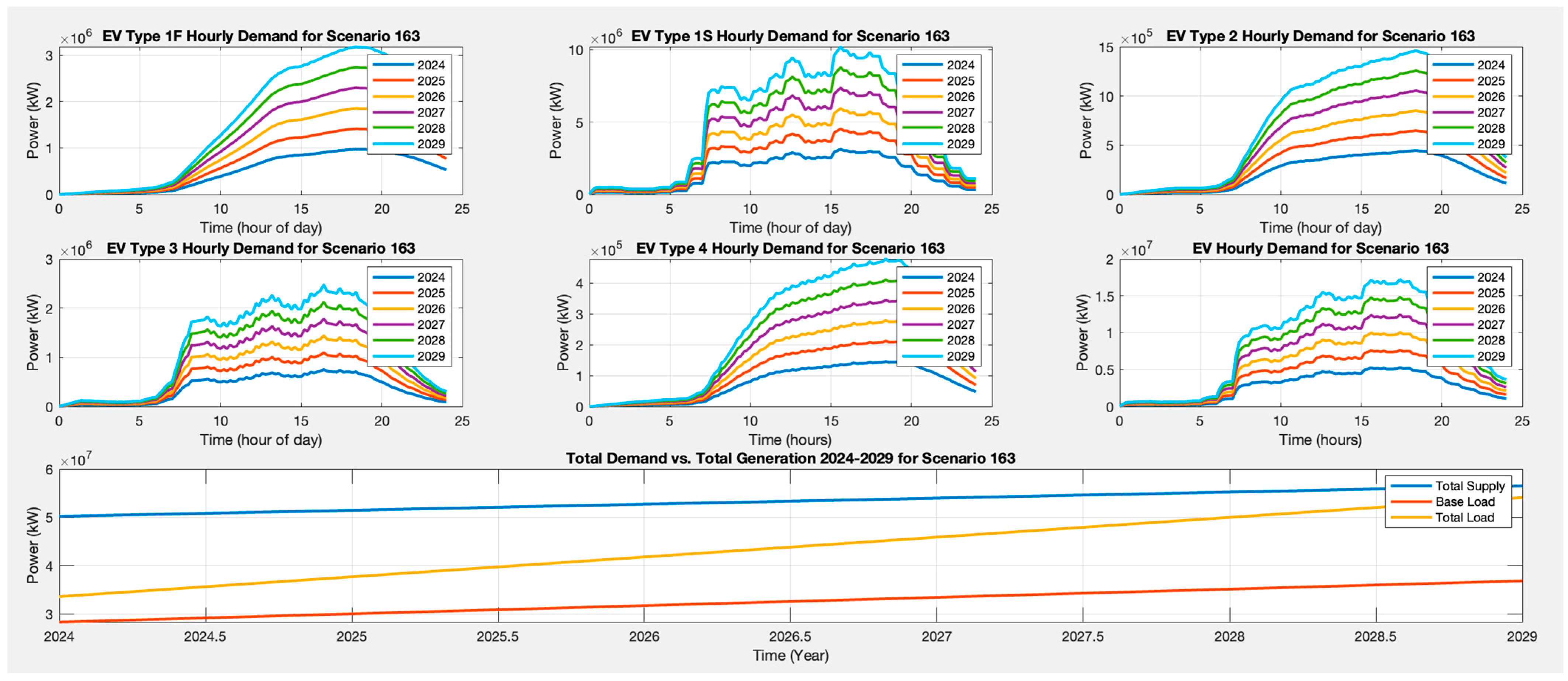
The worst-case scenario demonstrates that rapid and unregulated EV adoption, along with minimal subsidy impact and a preference for public charging, resulted in the lowest percentage of EV adoption and the highest annual allocation for EV subsidies. This scenario resulted in the supply and demand details presented in Table 13.
Table 13.
Worst Scenario Outputs.
The lack of synchronization between grid supply and demand will lead to a significant increase in EV subsidy costs required to maintain grid balance. The hourly demand for each EV type and the total power plant surplus are shown in Figure 14.
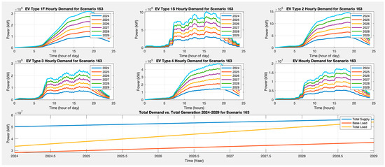
Figure 14.
Worst Scenario Output Graphs.
4.3. Most Probable Scenario
Another simulation result worth analyzing is the most probable scenario, as highlighted blue in Table 14. This scenario was determined based on information collected during the literature research. The growth of power plant capacity is expected to be slow due to PLN’s current oversupply issue [35]. Normal predictions are made for base peak load demand, personal vehicle population, and EV attractiveness growth [36]. According to a survey conducted by Indonesia Cerah in January 2024, subsidies are expected to have a high impact on EV attractiveness in Indonesia [37]. In the last year, there has been a strong preference for budget daily cars, reflecting the direction of the Indonesian market [38]. Home charging is strongly preferred over public charging [39].
Table 14.
Most Probable Scenario Inputs.
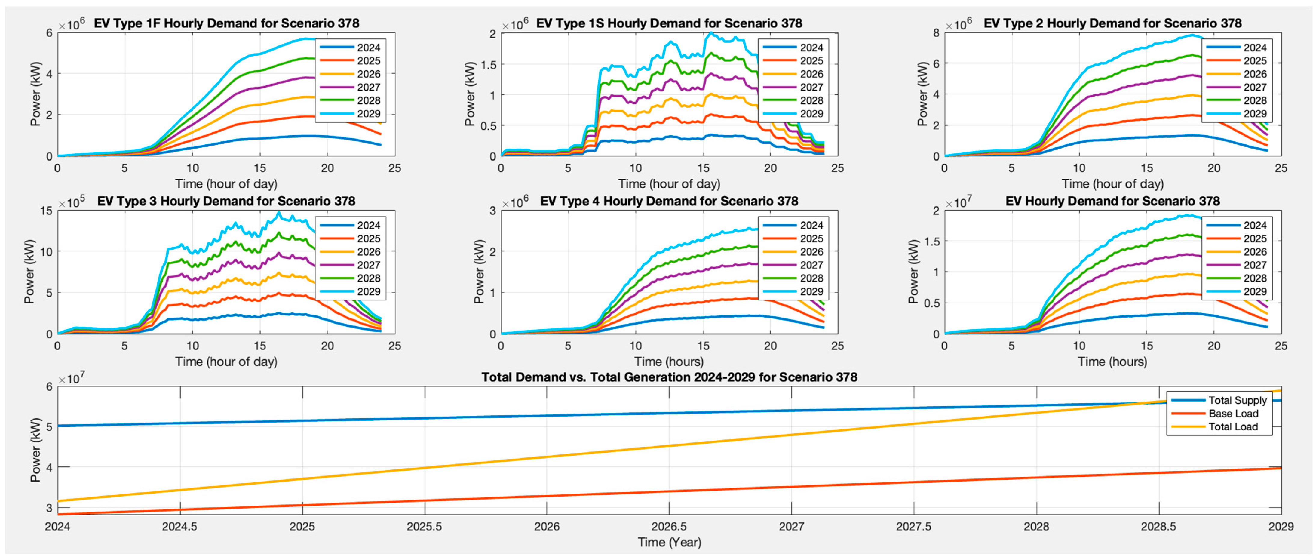
The scenario permutation of 1222333 (highlighted in blue) translates to the scenario labelled 378. This scenario resulted in a 42.98% EV percentage in 2029, as presented in Table 15. In that year, there is a power plant capacity deficit of 2397 MW. To achieve supply–demand balance, a cost allocation of Rp970,330,692,972 needs to be prepared.
Table 15.
Most Probable Scenario Outputs.
The most probable scenario unexpectedly resembles the best-case scenario, wherein the growth of both the supply and demand sides of the grid are relatively proximal synchronized. This outcome led to a lower annual cost allocation required to sustain the grid’s equilibrium. The hourly demand for each EV type and the total power plant deficit are presented in Figure 15.
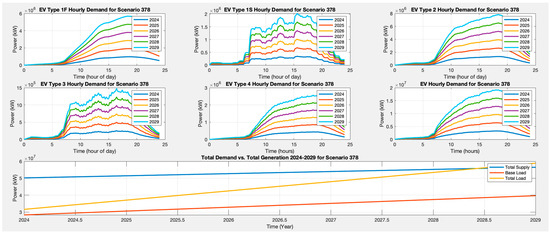
Figure 15.
Most Probable Scenario Output Graphs.
4.4. Least Probable Scenario
On the other hand, the least probable scenario, based on the literature review, features inputs that are the opposite of the most probable scenario. The inputs for scenario 1621 of 3111111 (highlighted in blue) are shown in Table 16.
Table 16.
Least Scenario Inputs.
Based on the literature research, the least probable scenario depicts a scenario where the grid’s supply grows significantly while EV adoption remains slow, with minimal subsidy impact and a preference for public charging. This scenario resulted in supply and demand details as outlined in Table 17.
Table 17.
Least Probable Scenario Outputs.
This scenario results in an imbalanced growth between the supply and demand sides of the grid, necessitating a substantial allocation of costs for EV subsidies to synchronize the grid’s supply–demand equilibrium. The hourly demand for each EV type and the total power plant surplus are shown in Figure 16.
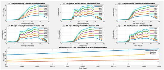
Figure 16.
Least Scenario Output Graphs.
4.5. Accuracy Checks
To ensure the accuracy of the results obtained from the model, several verification approaches have been implemented:
- Historical Data Validation: The model’s outputs have been compared against actual historical data on population growth, vehicle adoption rates, EV usage, and grid performance, as presented in Table 18. This comparison has helped identify any discrepancies and allowed for refinement of the model to improve accuracy.
Table 18. Accuracy Check Using 5-Year Supply Capacity Installed Historical Data.
- Sensitivity Analysis: Sensitivity analysis has been conducted to assess the model’s robustness by testing it under various assumptions and input scenarios, ensuring that the model remains reliable under different conditions.
- Expert Evaluation: The model has undergone evaluation by experts in the field, providing critical feedback.
By implementing these validation steps, the model is now suitable for developing development strategies with confidence in its accuracy and reliability.
5. Conclusions
The simulation outputs are intended to act as predictive guidelines for forecasting and implementing measures to sustain the supply–demand balance in Jamali’s power grid. This includes considerations for the growing presence of electric vehicles and the influence of subsidies.
According to the best-case scenario, achieving a high percentage of electric vehicles (EVs) by 2029 with minimal cost allocation necessitates a strategy of deliberate, gradual EV population growth, while maximizing the subsidy’s impact on EV attractiveness and encouraging home charging. In this simulation, vehicle preferences have a relatively minor impact on the output compared to the preferences for public versus home charging.
The worst-case scenario depicts the negative outcomes of rapid and unregulated EV growth, combined with a low subsidy impact and a strong preference for public charging. This scenario leads to a significantly low EV percentage by 2029 and a huge allocation of costs for subsidies. It serves as a cautionary example, emphasizing the criticality of strategic planning and policy implementation to guide EV adoption toward sustainable and balanced growth.
Due to limitations in data availability, variables such as dynamic population growth factors, dynamic peak load curves on weekends, and dynamic initial charging times (ICT) were not included in this simulation. These variables could be integrated into future improvements to enhance the model’s accuracy. Improving the simulation’s inputs and incorporating additional variables should markedly enhance its accuracy and utility.
Future work should focus on incorporating real-time data and exploring additional variables to further refine the model. This simulation could also serve as a foundation for a larger simulation addressing another significant change in the grid’s supply and demand, such as integrating solar panels into the supply side. Utilizing the scenario function of this simulation, scenarios could be simulated to assess the impact of different levels of solar panel penetration on the grid. Real-time data on energy production from photovoltaic systems can be incorporated as an input in the annual supply–demand simulation.
This paper presents a comprehensive simulation of the impact of EV growth on the grid’s supply–demand balance in the Jawa and Bali regions, addressing significant research gaps by incorporating dynamic growth factors and real-time data inputs. The findings and methodologies outlined not only provide valuable insights for current policy and infrastructure planning but also serve as a robust foundation for future developments in managing the integration of EVs into the power grid.
Author Contributions
Conceptualization, J.V.T. and R.D.; methodology, J.V.T. and R.D.; software, J.V.T.; validation, J.V.T. and R.D.; formal analysis, J.V.T. and R.D.; investigation, J.V.T. and R.D.; resources, J.V.T. and R.D.; data curation, J.V.T.; writing—original draft preparation, J.V.T.; writing—review and editing, J.V.T.; visualization, J.V.T.; supervision, R.D.; project administration, R.D.; funding acquisition, R.D. All authors have read and agreed to the published version of the manuscript.
Funding
This research was funded by Dissertation Research Grant for International Publication Universitas Indonesia (Hibah Riset PUTI UI) no. NKB-339/UN2.RST/HKP.05.00/2022.
Data Availability Statement
The original contributions presented in the study are included in the article, further inquiries can be directed to the corresponding author.
Acknowledgments
The authors would like to express their gratitude and appreciation to the Research and Development Department of the University of Indonesia (Risbang UI) for financing this study through the Dissertation Research Grant for International Publication (Hibah Riset PUTI UI) no. NKB-339/UN2.RST/HKP.05.00/2022.
Conflicts of Interest
The authors declare no conflicts of interest.
Appendix A. Simulation Input Excel Data
Figure A1 depicts a screenshot of an Excel table utilized as the initial input for the simulation, with adjustable inputs as needed [1,2,3,4,5,22,23,31,32].
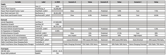
Figure A1.
Screen capture of the initial input excel data.
Figure A1.
Screen capture of the initial input excel data.
Appendix B. Results Data and Graphs
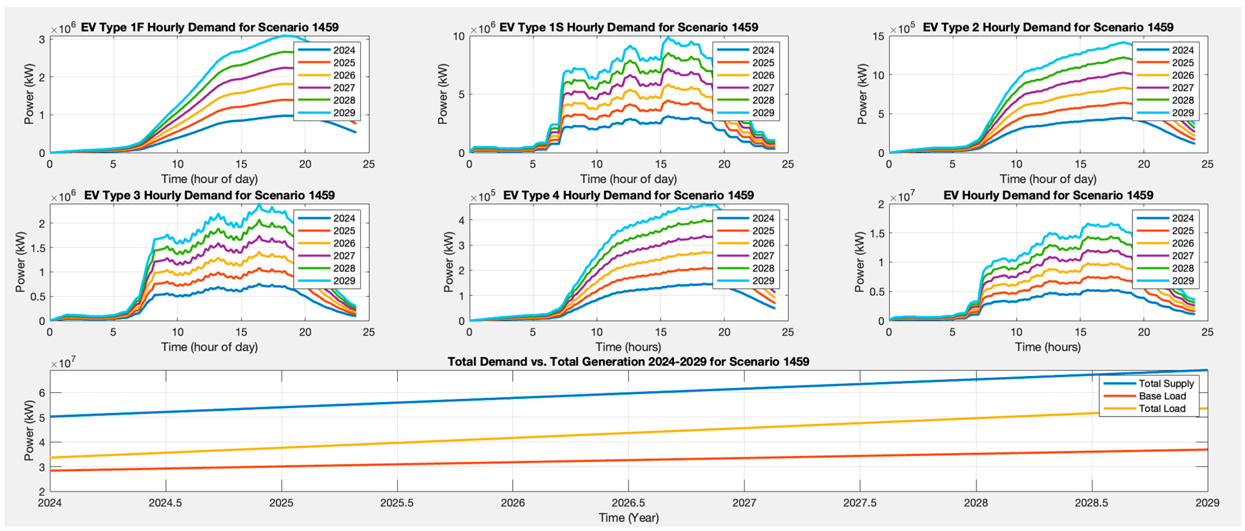
After each supply–demand simulation, the following output data could be displayed for further detail analysis. Figure A2 displays the hourly demand for each vehicle type in each year. It also shows the grid’s yearly total supply, yearly total demand, and yearly base load.
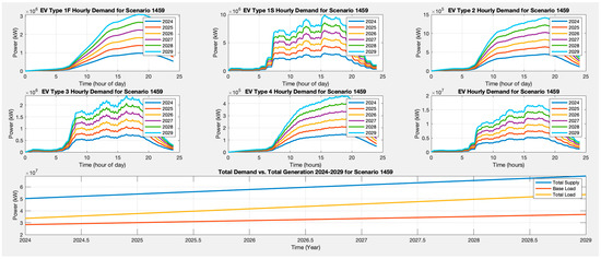
Figure A2.
Scenario Output Graphs.
Figure A2.
Scenario Output Graphs.
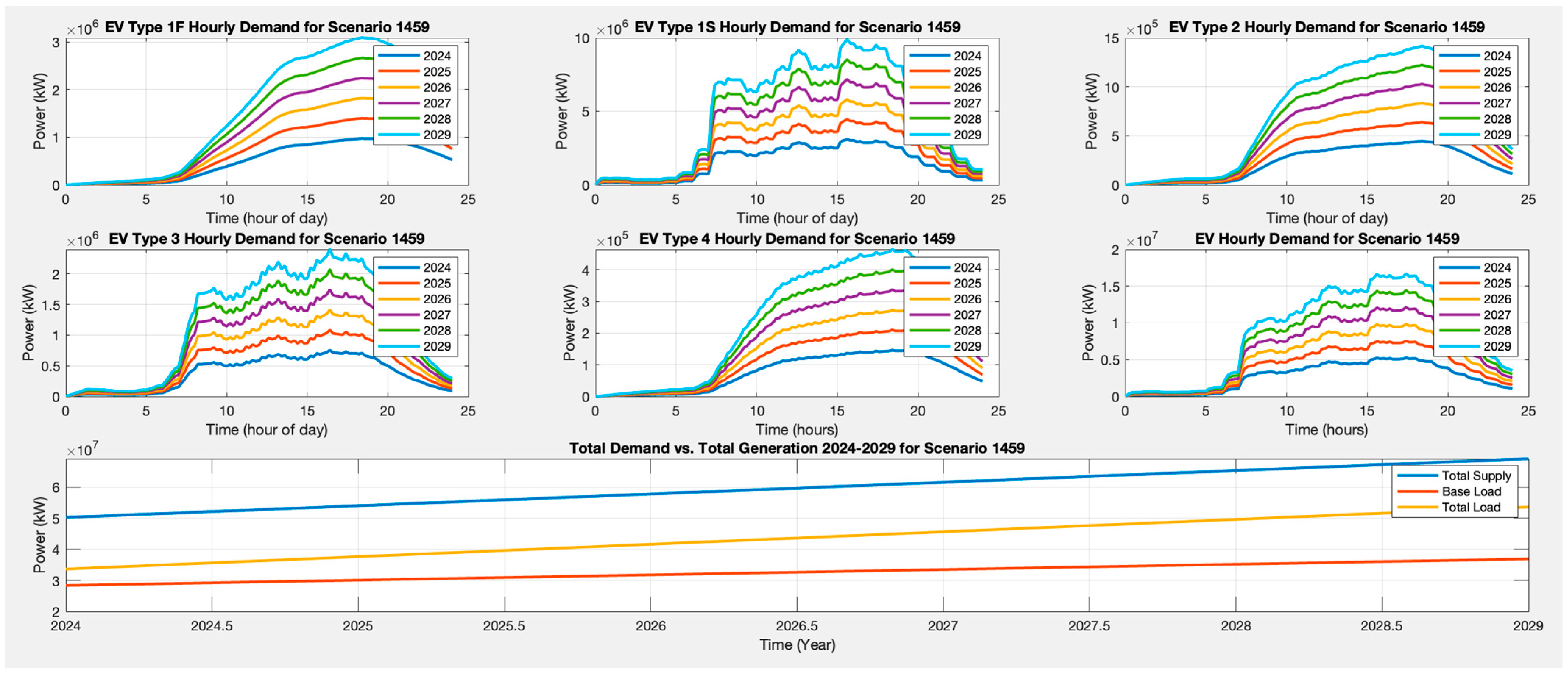
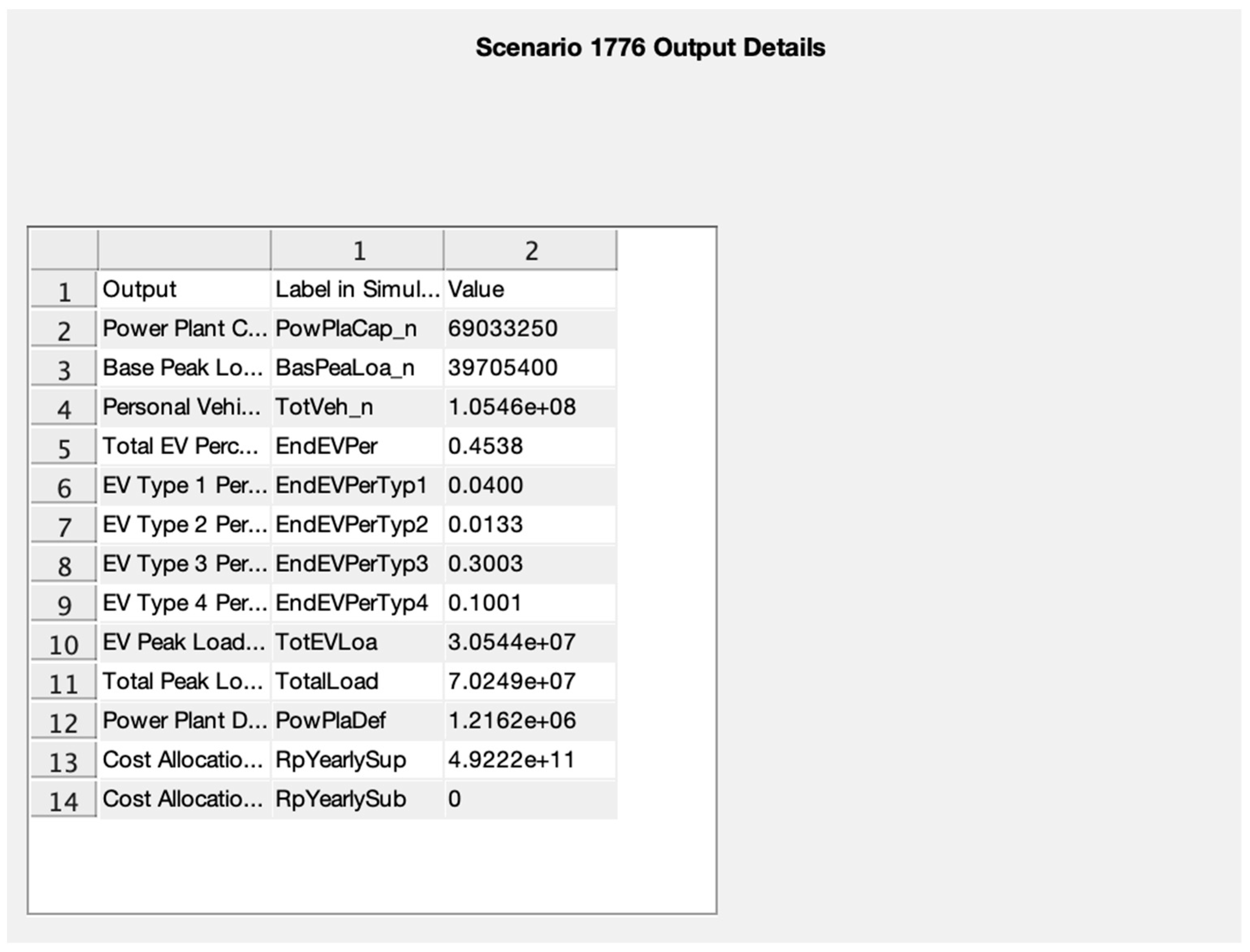
Figure A3 could also be displayed for each specific scenario, providing detailed output figures for further analysis.

Figure A3.
Scenario Output Details.
Figure A3.
Scenario Output Details.
Following the comprehensive scenario and supply–demand simulation, Figure A4 presents the three output factors, including EV percentage, annual supply cost allocation, and annual subsidy cost allocation, for the results sortation.

Figure A4.
Global Simulation Output Graphs.
Figure A4.
Global Simulation Output Graphs.
References
- PT. PLN (Persero). Statistik PLN 2023; PT. PLN (Persero): Jakarta, Indonesia, 2024; p. 1. [Google Scholar]
- Badan Pusat Statistik: Jumlah Kendaraan Bermotor Menurut Provinsi dan Jenis Kendaraan (Unit). 2022. Available online: https://www.bps.go.id/id/statistics-table/3/VjJ3NGRGa3dkRk5MTlU1bVNFOTVVbmQyVURSTVFUMDkjMw==/jumlah-kendaraan-bermotor-menurut-provinsi-dan-jenis-kendaraan--unit---2022.html?year=2022 (accessed on 8 May 2024).
- PT. PLN (Persero). Rencana Usaha Penyediaan Tenaga Listrik (RUPTL) 2021–2030; PT. PLN (Persero): Jakarta, Indonesia, 2021; pp. IV–2, V–4, V–154. [Google Scholar]
- Direktorat Jenderal Kependudukan dan Catatan Sipil. Laporan Tahun 2022; Direktorat Jenderal Kependudukan dan Catatan Sipil: Jakarta, Indonesia, 2022. [Google Scholar]
- PT. PLN (Persero). Statistik PLN 2014-2022; PT. PLN (Persero): Jakarta, Indonesia, 2015; pp. 1–3. [Google Scholar]
- Tambunan, H.B.; Hakam, D.F.; Prahastono, I.; Pharmatrisanti, A.; Purnomoadi, A.P.; Aisyah, S.; Wicaksono, Y.; Sandy, I.G.R. The Challenges and Opportunities of Renewable Energy Source (RES) Penetration in Indonesia: Case Study of Java-Bali Power System. Energies 2020, 22, 5903. [Google Scholar] [CrossRef]
- Pemerintah Pusat. Peraturan Presiden (Perpres) Nomor 79 Tahun 2023 tentang Perubahan atas Peraturan Presiden Nomor 55 Tahun 2019 Tentang Percepatan Program Kendaraan Bermotor Listrik Berbasis Baterai (Battery Electric Vehicle) untuk Transportasi Listrik; Pemerintah Pusat: Jakarta, Indonesia, 2023.
- The Association of Indonesia Automotive Industries. Indonesian Automotive Industry Data 2023; GAIKINDO: Jakarta, Indonesia, 2024. [Google Scholar]
- PT. PLN: Press Release No. 047.PR/STH.00.01/II/2024. Available online: https://web.pln.co.id/cms/media/siaran-pers/2024/02/lebih-dari-1-100-spklu-tersedia-pln-siap-layani-mobilitas-ev-di-hari-h-pemilu-2024/ (accessed on 5 May 2024).
- Pemerintah Daerah Khusus Ibukota Jakarta. Peraturan Gubernur (PERGUB) Provinsi Daerah Khusus Ibukota Jakarta Nomor 88 Tahun 2019 Tentang Perubahan Atas Peraturan Gubernur Nomor 155 Tahun 2018 Tentang Pembatasan Lalu Lintas Dengan Sistem Ganjil Genap; Pemerintah Daerah Khusus Ibukota Jakarta: Jakarta, Indonesia, 2019. [Google Scholar]
- Kementrian Keuangan. Peraturan Menteri Keuangan Nomor 10 Tahun 2024 tentang Perubahan Atas Peraturan Menteri Keuangan Nomor 26/PMK.010/2022 tentang Penetapan Sistem Klasifikasi Barang Dan Pembebanan Tarif Bea Masuk Atas Barang Impor; Kementrian Keuangan: Jakarta, Indonesia, 2024. [Google Scholar]
- Kementrian Perdagangan Republik Indonesia. Surat Edaran Nomor 03 Tahun 2023 tentang Penyediaan Stasiun Pengisian Kendaraan Listrik Umum dan Pemberian Tempat Parkir Prioritas Untuk Kendaraan Bermotor Listrik Berbasis Baterai (Battery Electrical Vehicle) di Pusat Perbelanjaan; Kementrian Perdagangan Republik Indonesia: Jakarta, Indonesia, 2023. [Google Scholar]
- Kementrian Keuangan. Peraturan Menteri Keuangan Nomor 38 Tahun 2023 tentang Pajak Pertambahan Nilai atas Penyerahan Kendaraan Bermotor Listrik Berbasis Baterai Roda Empat Tertentu dan Kendaraan Bermotor Listrik Berbasis Baterai Bus Tertentu yang Ditanggung Pemerintah Tahun Anggaran 2023; Kementrian Keuangan: Jakarta, Indonesia, 2023. [Google Scholar]
- Kementrian Perindustrian. Peraturan Menteri Perindustrian Nomor 6 Tahun 2023 Tentang Pedoman Pemberian Bantuan Pemerintah Untuk Pembelian Kendaraan Bermotor Listrik Berbasis Baterai Roda Dua; Kementrian Perindustrian: Jakarta, Indonesia, 2023. [Google Scholar]
- Pemerintah Pusat. Undang-undang (UU) Nomor 42 Tahun 2008 tentang Pemilihan Umum Presiden dan Wakil Presiden; Pemerintah Pusat: Jakarta, Indonesia, 2008; p. 5. [Google Scholar]
- Zulfiqar, M.; Alshammari, N.F.; Rasheed, M.B. Reinforcement Learning-Enabled Electric Vehicle Load Forecasting for Grid Energy Management. Mathematics 2023, 11, 1680. [Google Scholar] [CrossRef]
- Feng, J.; Chang, X.; Fan, Y.; Luo, W. Electric Vehicle Charging Load Prediction Model Considering Traffic Conditions and Temperature. Processes 2023, 11, 2256. [Google Scholar] [CrossRef]
- Khan, W.; Somers, W.; Walker, S.; de Bont, K.; Van der Velden, J.; Zeiler, W. Comparison of electric vehicle load forecasting across different spatial levels with incorporated uncertainty estimation. Energy 2023, 283, 129213. [Google Scholar] [CrossRef]
- Jaruwatanachai, P.; Sukamongkol, Y.; Samanchuen, T. Predicting and Managing EV Charging Demand on Electrical Grids: A Simulation-Based Approach. Energies 2023, 16, 3562. [Google Scholar] [CrossRef]
- Umair, M.; Hidayat, N.M.; Ali, N.H.; Abdullah, E.; Johari, A.R.; Hakomori, T. The effect of vehicle-to-grid integration on power grid stability: A review. IOP Conf. Ser. Earth Environ. Sci. 2023, 1281, 012070. [Google Scholar] [CrossRef]
- Lu, D.; Lu, Y.; Zhang, K.; Zhang, C.; Ma, S.C. An Application Designed for Guiding the Coordinated Charging of Electric Vehicles. Sustainability 2023, 15, 10758. [Google Scholar] [CrossRef]
- Badan Pusat Statistik: Perkembangan Jumlah Kendaraan Bermotor Menurut Jenis (Unit), 2021–2022. Available online: https://www.bps.go.id/id/statistics-table/2/NTcjMg==/perkembangan-jumlah-kendaraan-bermotor-menurut-jenis--unit-.html (accessed on 6 April 2024).
- Kementrian Perhubungan. Populasi Kendaraan Listrik di Indonesia berdasarkan Registrasi Uji Tipe; Kementrian Perubungan: Jakarta, Indonesia, 2023. [Google Scholar]
- Wang, H.J.; Wang, B.; Fang, C.; Li, W.; Huang, H.W. Charging Load Forecasting of Electric Vehicle Based on Charging Frequency. IOP Conf. Ser. Earth Environ. Sci. 2019, 237, 062008. [Google Scholar] [CrossRef]
- Hyundai Ioniq Specification. Available online: https://www.hyundai.com/id/id/find-a-car/ioniq5/specification (accessed on 1 April 2024).
- Khairunisa, W.A.; Munandar, A. The Commuting Pattern Analysis of Commuters from Depok City West Java. J. Spat. Wahana Komun. Dan Inf. Geogr. 2020, 20, 1–9. [Google Scholar]
- Inside EV: Hyundai Ioniq 5 Amazes: Real Fast Charging Session Data Analyzed. Available online: https://insideevs.com/news/503522/hyundai-ioniq5-fast-charging-analysis/ (accessed on 3 April 2024).
- Wuling Air Specification. Available online: https://wuling.id/id/air-ev?product_id=18 (accessed on 5 April 2024).
- United TX1800 Specification. Available online: https://unitedmotor.co.id/product/tx1800/ (accessed on 5 April 2024).
- Viar New Q1L Specification. Available online: https://viarmotor.com/subsidi-motor-listrik-viar-new-q1/ (accessed on 5 April 2024).
- Sefriyadi, I.; Andani, I.G.A.; Raditya, A.; Belgiawan, P.F.; Windasari, N.A. Private car ownership in Indonesia: Affecting factors and policy strategies. TRIP Transp. Res. Interdiscip. Perspect. 2023, 19, 100796. [Google Scholar] [CrossRef]
- Bloomberg Newsletter: Electric Vehicle Market Looks Headed for 22% Growth This Year. Available online: https://www.bloomberg.com/news/newsletters/2024-01-09/electric-vehicle-market-looks-headed-for-22-growth-this-year (accessed on 1 May 2024).
- Uspensky, J.V. Introduction to Mathematical Probability; McGraw-Hill: New York, NY, USA, 1937. [Google Scholar]
- PT. PLN (Persero). Statistik PLN 2021; PT. PLN (Persero): Jakarta, Indonesia, 2022; p. 77. [Google Scholar]
- Hamdi, E.; Adhiguna, P. Indonesia Wants to Go Greener, but PLN Is Stuck with Excess Capacity from Coal-Fired Power Plants; IEEFA: Lakewood, OH, USA, 2021; pp. 2–4. [Google Scholar]
- Jones, G.W. The 2010–2035 Indonesian Population Projection; UNFPA: Jakarta, Indonesia, 2014. [Google Scholar]
- Indonesia Cerah. Survey Kebijakan Transisi Energi Berkeadilan; Yayasan Indonesia Cerah: Jakarta, Indonesia, 2024. [Google Scholar]
- VERO. The Road to Southeast Asia. Available online: https://vero-asean.com/whitepaper/chinese-automotive-in-southeast-asia/ (accessed on 28 June 2024).
- IESR. Indonesia Electric Vehicle Outlook 2023; IESR: South Jakarta, Indonesia, 2023; p. 27. [Google Scholar]


Disclaimer/Publisher’s Note: The statements, opinions and data contained in all publications are solely those of the individual author(s) and contributor(s) and not of MDPI and/or the editor(s). MDPI and/or the editor(s) disclaim responsibility for any injury to people or property resulting from any ideas, methods, instructions or products referred to in the content. |
© 2024 by the authors. Licensee MDPI, Basel, Switzerland. This article is an open access article distributed under the terms and conditions of the Creative Commons Attribution (CC BY) license (https://creativecommons.org/licenses/by/4.0/).