Abstract
This article presents the instrumentation of an electronic–mechanical differential prototype, consisting of an arrangement of three throttles to operate two hub motors on the rear wheels of an electric vehicle. Each motor is connected to its respective throttle, while a third throttle is connected in series with the other two. This configuration allows for speed control during both rectilinear and curvilinear motion, following Ackermann differential geometry, in a simple manner and without the need for complex electronic systems that make the electronic differential more expensive. The differential throttles are strategically positioned on the mass bars connected to the steering system, ensuring that the rear wheels maintain the appropriate differential ratio. For this reason, it is referred to as an “electronic–mechanical differential”. Additionally, this method can be extended to a four-wheel differential system.
1. Introduction
Today, the automotive industry is facing one of the greatest challenges in its history: there is an urgent need to adopt innovative and effective solutions that drastically reduce environmental impact and contribute toward the fight against climate change. Many companies are joining this noble cause through contributions such as the development of electric vehicles (EVs), hybrids, and more efficient and cleaner propulsion systems. Although significant progress has been made, there is still a long way to go to achieve truly sustainable and environmentally friendly mobility and transport.
As for EVs, research efforts have concentrated on every part of the vehicle, from the lithium-ion battery [1] to the mechanical transmission of the vehicle [2]; therefore, it is of the utmost importance to consider the energy autonomy of EVs, in which the body, chassis, and transmission of the vehicle are involved.
In particular, the transmission requires a differential that allows for the rotation of the wheels to be controlled according to the curve of the road. When an engine is used that provides the transmission of the movement through an axle, as is classically presented in internal combustion (IC) vehicles, a mechanical differential (MD) is required, generally consisting of a gear formed by a crown and satellite pinions, which allows for differentiating the movement of one wheel with respect to the other, depending on the requirements of the curve of the road [2].
With the advent of EVs, the MD is still functional; however, in recent years, the use of hub motors for EV propulsion has been proposed. In general, hub motors are positioned in the rims of the tires; therefore, the mechanical differential is no longer directly functional, and either adjustments or a move of what is known as the electronic differential (ED) must be made.
In [3], the main objective of the work was to implement a vehicle differential mechanism using electronic means. Measuring the actual wheel speed and estimating the required speed of the direct current (DC) motor are both necessary to generate the appropriate control signal for achieving the desired speeds on different wheels. The motor shaft is connected to an optical encoder, which converts the speed into a train of TTL-compatible pulses. This pulse train is then fed to the frequency-to-voltage converter (FVC), a technique that is typical of electronic differentials (EDs).
In this context, we propose the instrumentation of an electronic differential for hub motors (HMs) used for the propulsion of an EV, basically making an arrangement of commercial throttles and controllers. For the reasons presented here, it is called the electrical–mechanical differential (DEM) because the instrumentation of commercial electronic components requires it to be implemented in an ingeniously mechanical way for their corresponding drive. This arrangement, implemented in a prototype, was proved to be both efficient and significantly more economical than the ED, as it eliminates the need for complex electronics, such as encoders and data processors, to correlate the rotation of the front tires in a curve with the rotational speed of the rear tires.
2. Background
Research centers at universities and laboratories have been dedicated to EV research, some concentrating on the optimization of the electric motor (EM). In general, there is an evolution taking place in terms of the change from internal combustion engines to electric motors in automobiles, an evolution that dates back to 1832 and is almost on par with the evolution of the internal combustion engine.
There are five types of EM suitable for electromobility: induction motors, direct-current motors, synchronized permanent magnet motors, BLDC motors, and switched reluctance motors [2,4]. BLDC motors are the most popular in electromobility, while the induction motor is the most advanced technology for EV applications [5]. BLDC motors weigh less and are smaller than a brush motor that has equal power, making them ideal for reducing space [6]. Thus, HMs allow for more space for passengers and simplify the mechanics of the car, improving handling [6] and making them suitable for urban use. Additionally, an HM on each wheel is controlled independently [7]. HMs are used in bicycles, motorcycles, scooters, solar cars, and many other lightweight EVs [8,9]. These EVs are practical, economical, and eliminate environmental pollution, and, due to their manufacturing size, they also reduce road congestion in cities.
A three- or four-wheeled vehicle requires a differential to ensure that the speed of each wheel is controlled. The equations of the Ackermann model are used to achieve this purpose [8,10]. An ED can be implemented regardless of the type of motor applied. In [11,12], traction control is reported using induction motors. Haddoun [11] used a dSPACE-type embedded system to calculate speed of the rear wheels. A Tabbache traction system was also reported [12] for which an algorithm based on a speed observer and adaptive flow was used, allowing for torque control, all in order to ensure stability of the vehicle in curves.
In [13], the design and evaluation of an ED system are reported, with four independent HMs. There are three driven configurations: front, rear, and four-wheel; there is a great versatility in controlling the axles and the wheels.
For example, an ED design, with a system with BLDC motors in each wheel of 15 kW in a Fiat vehicle, is given in [14]. Another implementation of a differential with three-phase commercial motors, with a squirrel cage rotor, which were rewound to operate with 28 Vrms of line while maintaining their original power, is presented in [15]; in the said works, an electronic arrangement was made to implement a DE with a single controller. An ED applied in BLDC motors and that does not require specific sensors to measure the steering angle or speed sensors, as implemented in an electric tricycle, is presented by Clavero in [16].
It should be mentioned that BLDC motors have a counter-electromotive force that is not sinusoidal; rather, it is trapezoidal, and due to the difference in its waveform with the stator currents, a ripple is created in the torque, which in turn creates speed fluctuations, vibration, and acoustic noise in the motor. Similarly, in [17], a ripple-free torque controller for a BLDC motor is proposed, which is also tolerant of phase faults.
The drive systems of EVs are divided into two groups: single-drive systems and multi-drive systems. The single-drive system consists of a high-speed motor, reduction gears, clutch, gearbox, and a differential; this type of drive reduces the efficiency of the EV due to the mechanical parts. In multiple-drive systems, each of the vehicle wheels is driven with a high-torque EM, and, in this way, mechanical parts are eliminated and efficiency increases [9]. The second system has a high-speed motor; therefore, reduction gears, a clutch, a gearbox, and a differential are required; thus, the efficiency of the EV is reduced due to the number of mechanical parts required. However, in the multiple-drive system, the differential behavior of the vehicle’s wheels during curves must be controlled, requiring an ED; that is, a technological device is required for curves. The wheels of the same axle rotate at different speeds to prevent one of them from skidding and losing traction. Meanwhile, on straight roads, the two tires must roll at the same speed by means of electronic control for each wheel, replacing the traditional planetary gear differential [2,16].
In most of the works, the simulation of the electronic differential was conducted using Simulink R2024b software from Matlab, [7,18,19,20,21]. In [18], a comparison is also made with Codesys simulation software. In [3], electronic instrumentation using MOSFETs was used for the simulation, presenting both theoretical and experimental results; the optical encoder was attached to the motor shaft, converting the motor’s speed into a pulse train with a frequency corresponding to the motor’s RPM. The encoder used in this setup generated 36 pulses per revolution. A frequency-to-voltage converter IC, LM2907, was employed to produce a 5V analog signal at the motor’s maximum speed. The microcontroller used was the AT89S52, which was interfaced with an 8-bit A/D converter IC, ADC0809.
In [22], an FPGA card with Verilog and HDL programming was used to achieve practical results, comparing them with the simulation of the torque results in Simulink-Matlab. Also, in [23], the electronic differential utilized the steering wheel command signal, throttle position signals, and engine speed signals to regulate the power supplied to each wheel, ensuring that all wheels received the necessary torque. The proposed control structure was based on PID control for each wheel motor. Subsequently, the performance of the PID control system was assessed in the Matlab-Simulink environment.
In order to calculate the speed of each wheel, an Ackermann-type model is suitable. The ED makes the use of this model, as the angular velocity of each wheel is calculated using the desired steering angle and reference speed. All wheels are required to have the same turning radius to apply in this model.
3. Materials and Methods
The innovation of the ED proposed herein is its skillful simplicity, since it can be directly implemented with commercial accessories: controllers and accelerators. The proposed implementation, unlike others [14,16], has an arrangement of three accelerators driven by the steering linkage in order to obtain the ratio of the rear tires of the EV after calculating the relationship between the speed and rotation of the vehicle according to Ackermann’s geometry.
The methodology for the instrumentation of the DEM differential is for an EV with rear-wheel drive and is based on two hub motors installed, one in each wheel, with independent controllers, and an arrangement of three accelerators connected in parallel series and mechanically implemented between the mass of the tires and the fixed part of the EV chassis. This instrumentation can be easily extended to the use of four or more pairs of engines, one HM for each tire. Therefore, the elements used in the EV is first described for the implementation of a DEM and then the methodology of the calculations necessary to form the control relationship is discussed. Also, the accessories, including hub motors, controllers, and throttles, are described below.
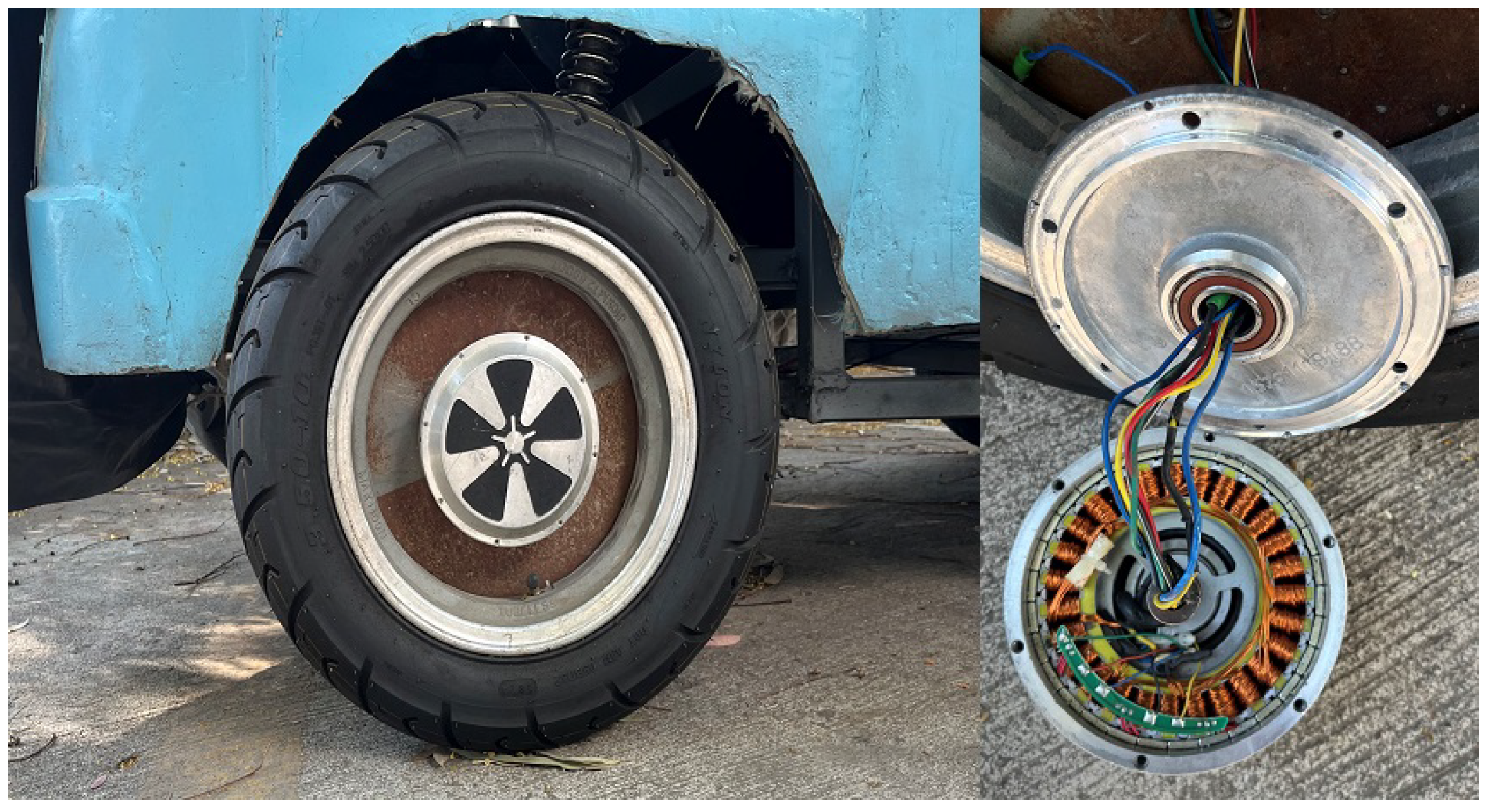
3.1. Hub Motors
In IC-to-EV conversion vehicles or even in some EVs, the engine throttles the power to the mechanical transmission called the “gearbox”; in its two modalities, the system has an integrated differential or the system that transmits power to an external differential. A different proposal from the former scheme is to transmit power directly to the rims using an HM; this is generally a brushless DC motor-type BDCL, (see Figure 1), with the external rotor and stator attached to the wheel axle, which remains fixed to the EV chassis. The rotor is thus connected directly to the rim of the wheel [8].
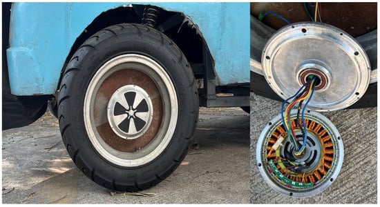
Figure 1.
Hub motor-type BDCL.
This is a 350 W motor that has an aluminum casing and a rotor with a 13 cm external diameter, operates at 36 V, is placed on a rim for a 40 cm diameter wheel, turns at maximum speed at an EV speed of 50 KM/h. The motor has 5 wires for Hall sensors for positioning magnetic fields and 3 power wires for three-phase rotor supply power.
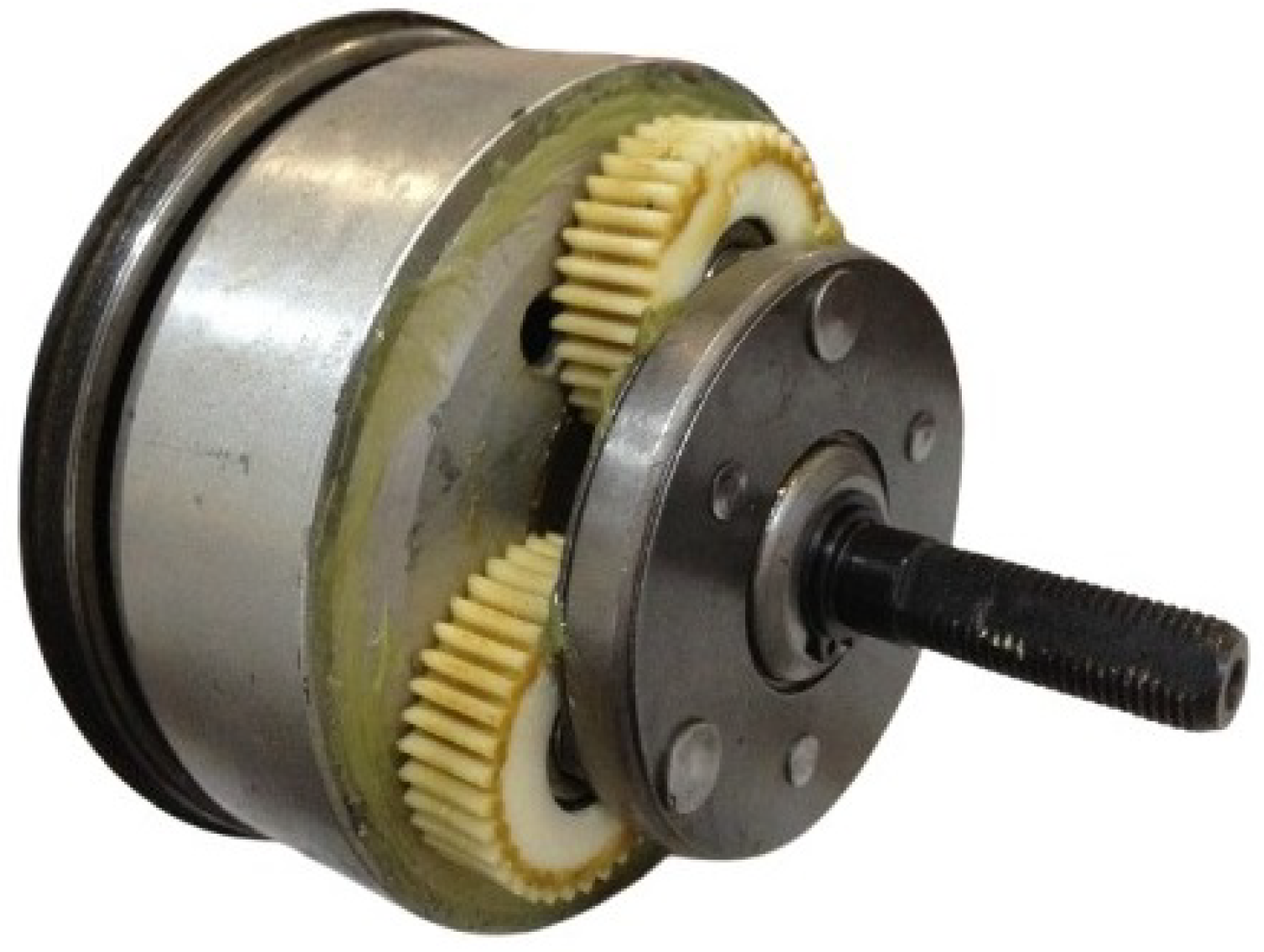
One of the first attempts to produce a DM to be applied to EVs moved with an HM had a planetary gear differential that sent the rotation of the external rotor of the high-speed BLDC motor directly to the wheel rim (see Figure 2), decreasing the output speed; however, this action increased the mass of the wheel, which did not to affect if an arrangement with a larger suspension damping was implemented.
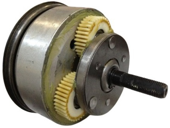
Figure 2.
Hub motor with gears.
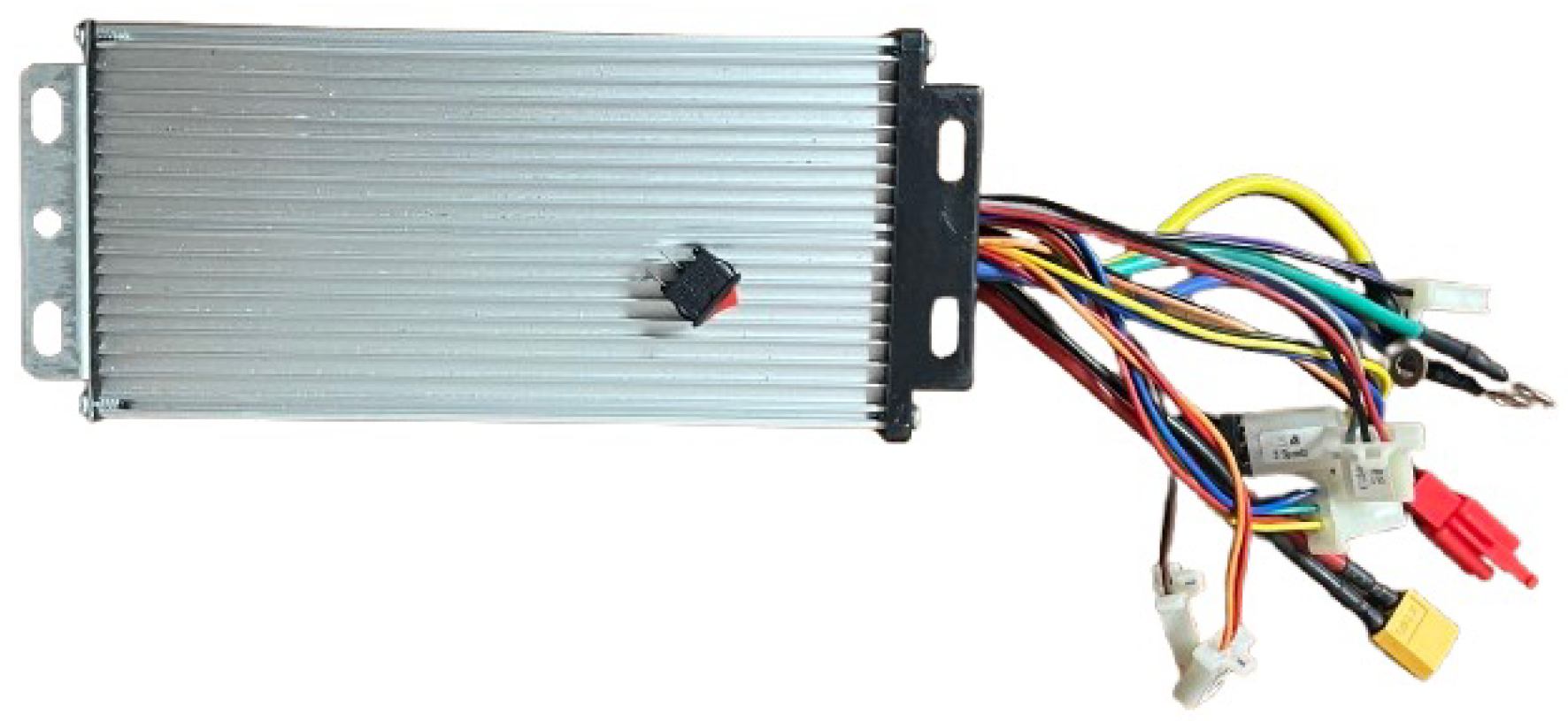
3.2. Controllers
Each BDCL-type motor uses a controller to regulate the speed (see Figure 3). In this case, two controllers are used, each with an operating voltage of 36 to 48 V, with a 5-wire connector to the Hall sensors for position and speed control, a 3-wire connector for three-phase power supply within the HM motor, a two-wire input connector for power to the 36 V battery, a 3-wire output connector to connect a throttle that operates at 4.5 V, a pair of output wires that interconnects with reverse motion, and several cables with their respective connectors for accessories such as switches, speakers, lights, etc.
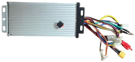
Figure 3.
Direct-current controller.
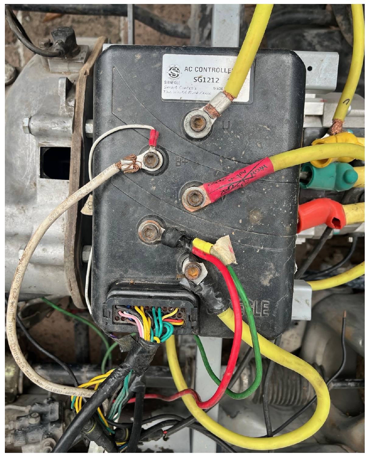
These controllers, unlike the controllers for alternating-current (AC) motors for EVs, do not have an integrated DC-to AC-inverter, as shown in Figure 4.

Figure 4.
Alternating-current controller.
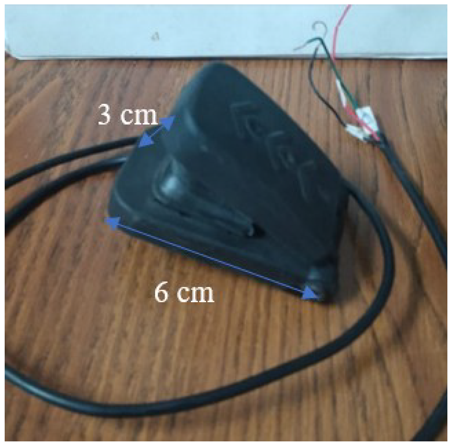
3.3. Accelerators
The implementation of a DEM requires three electronic pedal accelerators, Figure 5, which usually work at 4.5 V as a nominal voltage. They consist practically of a potentiometer that makes the current vary from 0 to 4.5 V; this voltage variation translates in the controller into a variation in the operating current on the motor from 0 to the maximum speed current.
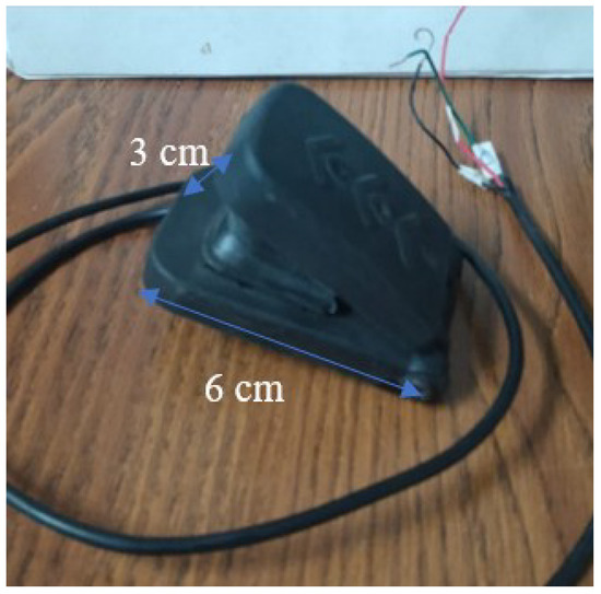
Figure 5.
Electric throttle pedal for EVs.
The throttle has a 3-wire connector that must be connected to the controller. This is common in a two-wheeled EV where no electronic differential is required, such as in a motorcycle, bicycle, or scooter.
In the implementation of a DEM, three accelerator pedals are required: one is directly instrumented, which would serve as the normal accelerator of the system. Two other accelerators are used, which must be connected to their respective controllers. These throttles are specially instrumented on the mass lever, which is connected to the steering rod and the axle, which is connected to the chassis. The series–parallel electrical connection between the accelerators is described below.
3.4. Calculations of Speed Ratios
Generally speaking, a DEM uses the Ackermann principle, which shows the four tires rolling around a common point called the “center of turning radius”, this situation occurs when the projection of the front wheel axles intersects with the projection of the rear axle line [7].
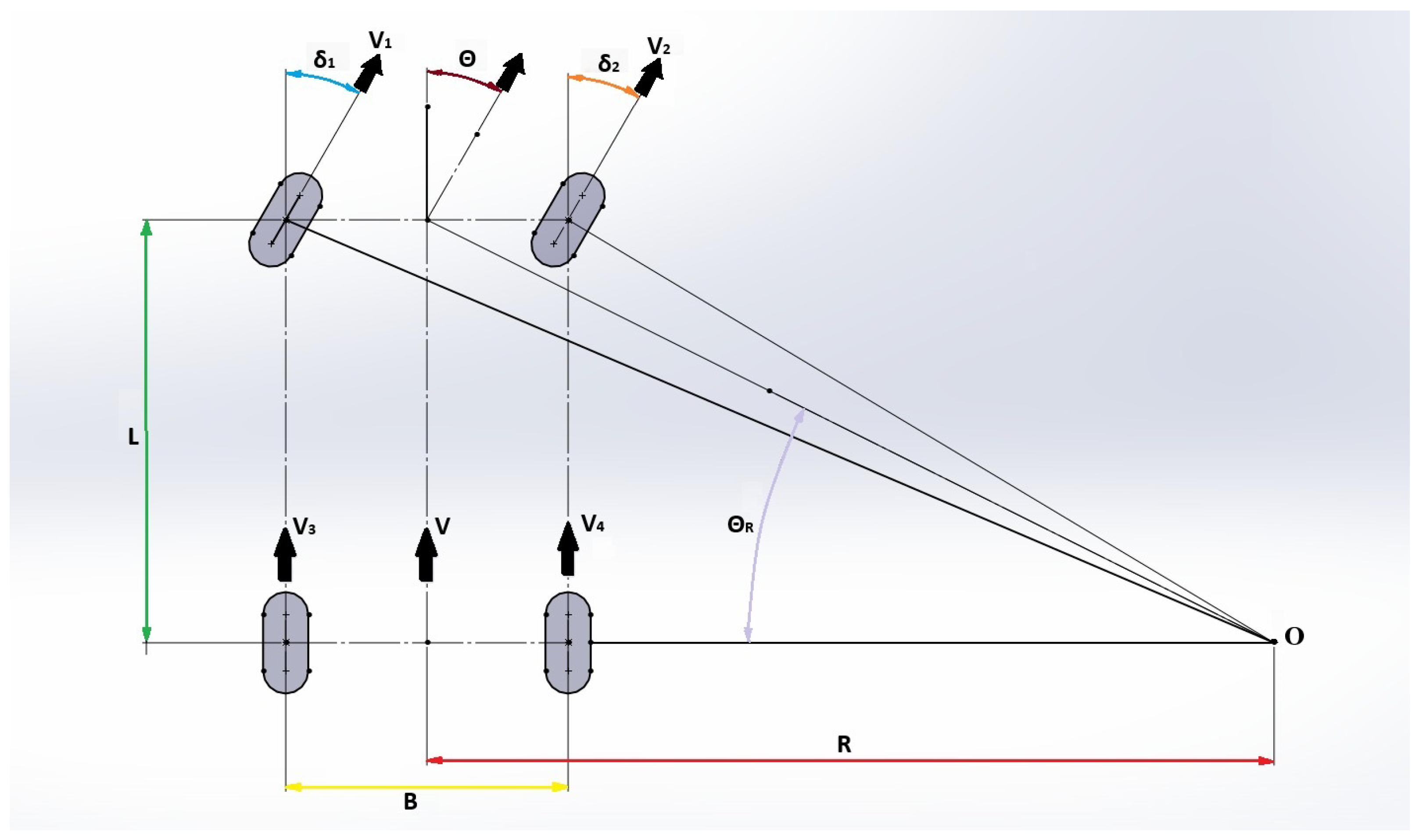
According to Ackermann’s model, Figure 6 depicts a four-wheeled vehicle turning right on a sharp curve, where V is the speed of the vehicle; V1, V2, V3, and V4 are the speeds of each of the wheels; and are the angles of each front wheel; R is the turning radius of the vehicle; L is the distance between the front and rear axles; B is the wheel separation distance; and O is the center of the turning radius.
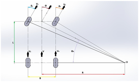
Figure 6.
Scheme of Ackerman geometry.
Note that the front tire of the vehicle, which is closer to the center, does not turn enough when the Ackermann angle is too small; it also causes understeer since the wheels do not have the same arch, which counteracts their movement, so they turn at unsynchronized angles. On the other hand, if there is too much angle, the inside rim drags.
Then, the speed of each wheel is calculated using the steering wheel steering angle and desired vehicle speed according to Ackermann’s model. From Moazen [7], the following equations were obtained, which we use to describe the SDE based on the Ackermann model.
The speed of the rear wheels is determined as a function of the yaw angular velocity with respect to O and the turning radius R; that is,
Then
where B is the distance between the rear tires, r is the radius of each wheel, and are the angular velocities of the rear tires.
This relationship implies that when , the speeds of the two wheels are almost equal; this occurs in rectilinear mode. In the case of 4 motors, that is, rim motors 1 and 2, the speeds are as followsing:
And, their respective angular velocities are
where L is the length between the axles of the VE; and are the angular velocities of the rear tires. Unlike [18,21], the analysis shown here clearly demonstrates that the speed of the internal wheels is lower than that of the external wheels, as the angles , as can be seen Figure 6.
On the other hand, the angles and of the front tires are determined by
Then, combining Equations (4) and (6) with Equations (5) and (7), respectively, we obtain the following:
Combining these equations, we obtain the proportion of the angular velocity with respect to ; that is
In the case of 4 HMs, if we want to maintain this speed relationship, we must also work in a direction that allows us to obtain angles and of the front tires according to Ackermann geometry. In [24], a parameter configuration with a rack direction is presented that allows achieving the Ackerman geometry.
For the case of only 2 HMs in rear-wheel drive, the angular relationship of the wheels can also be expressed in terms of angles and of the front tires; by substituting Equations (6) and (7) into Equation (3), we obtain
Also, from Figure 6, the following can be obtained:
In this way, it is possible to mechanically control the gear ratio of the rear tires to turn right by controlling angle of the front left rim. In a similar way, we proceed to apply the same process to turn left with angle . This can be achieved with a throttle connected in series to the controllers of the rear-wheel HMs.
Define
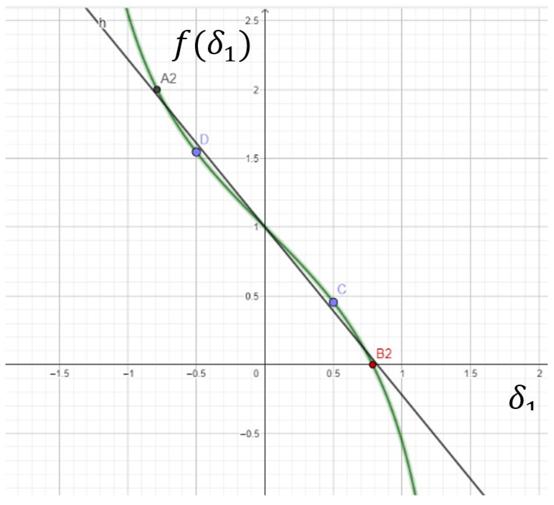
as a velocity multiplicity factor (FMV). The graph in Equation (10) for B/L = 1 (in green) is as follows:
In Figure 7, the line in black corresponds to the linear regression between the points: {((0.79, 0), (−0.79, 2), (0.5, 0.45), (−0.5, 1.55))}. This line obeys the following equation:
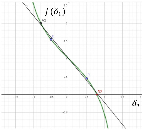
Figure 7.
Ratio of angular velocity to from wheel rotation in Equation (10) with B/L = 1.
The points on this line very accurately match those of the graph of Equation (11) between the inflection points. To obtain the inflection point, we derive Equation (11) and set it equal to 0; that is,
Consequently, , which implies that at , f changes its concavity.
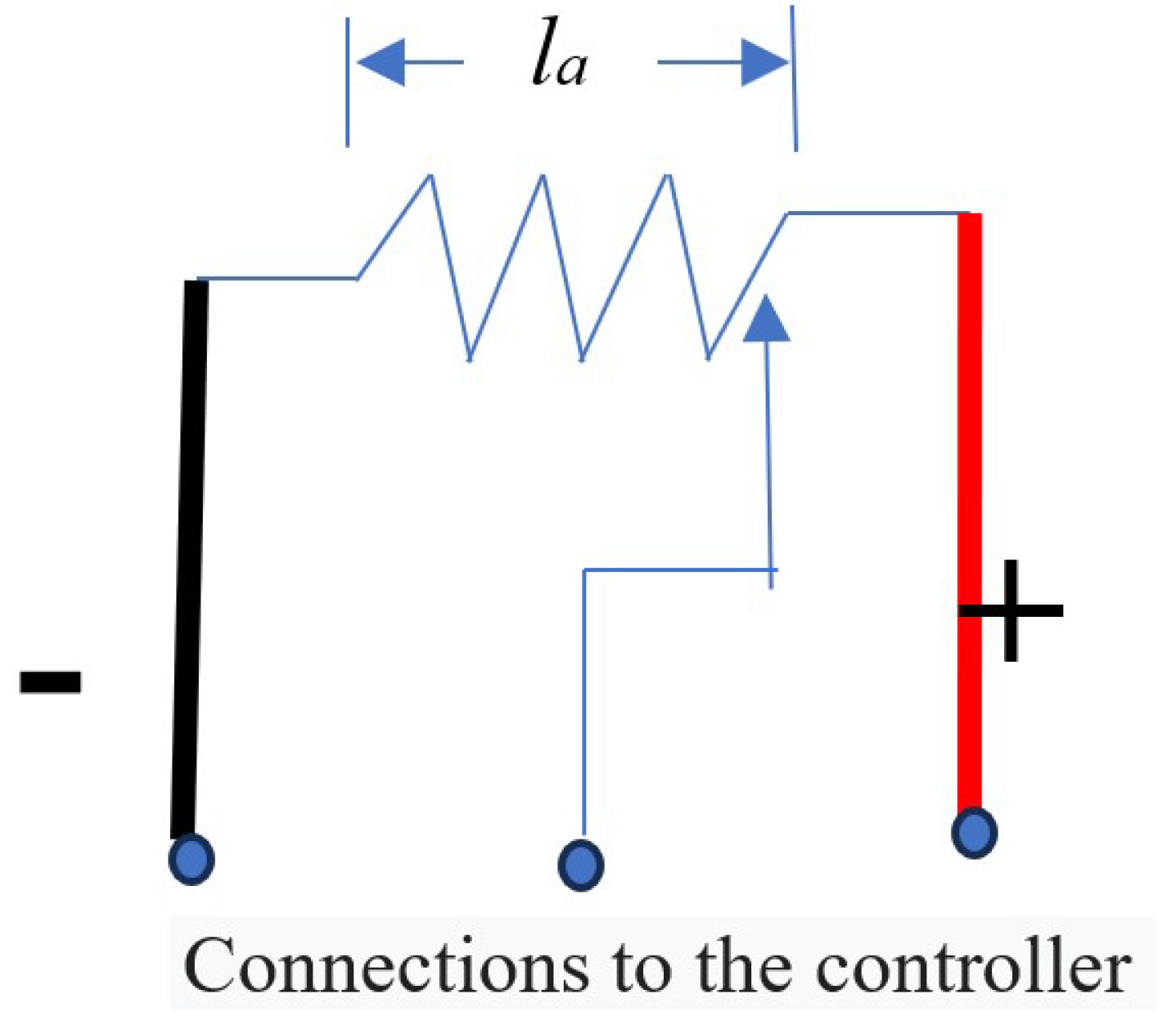
On the other hand, the accelerator pedal, together with the controller, makes the angular velocity of the tire linearly proportional to the stroke of the potentiometer resistance, as shown in Figure 8.
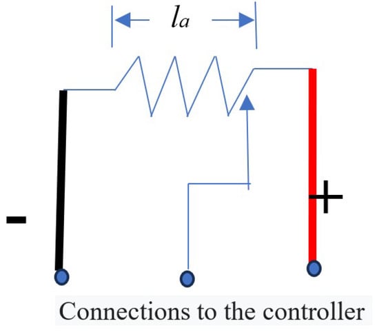
Figure 8.
Basic electric throttle circuit.
To relate the movement of the levers of the masses, which connect to the steering system (SD), with the pedal accelerator arms, let be the radius that corresponds to a fraction of the lever of the mass of the tire, which engages the SD, and let be the opening of the throttle hinge. The above description defines the electronic differential, and the calculations necessary for its strategic location are described below.
3.5. Electronic–Mechanical Differential
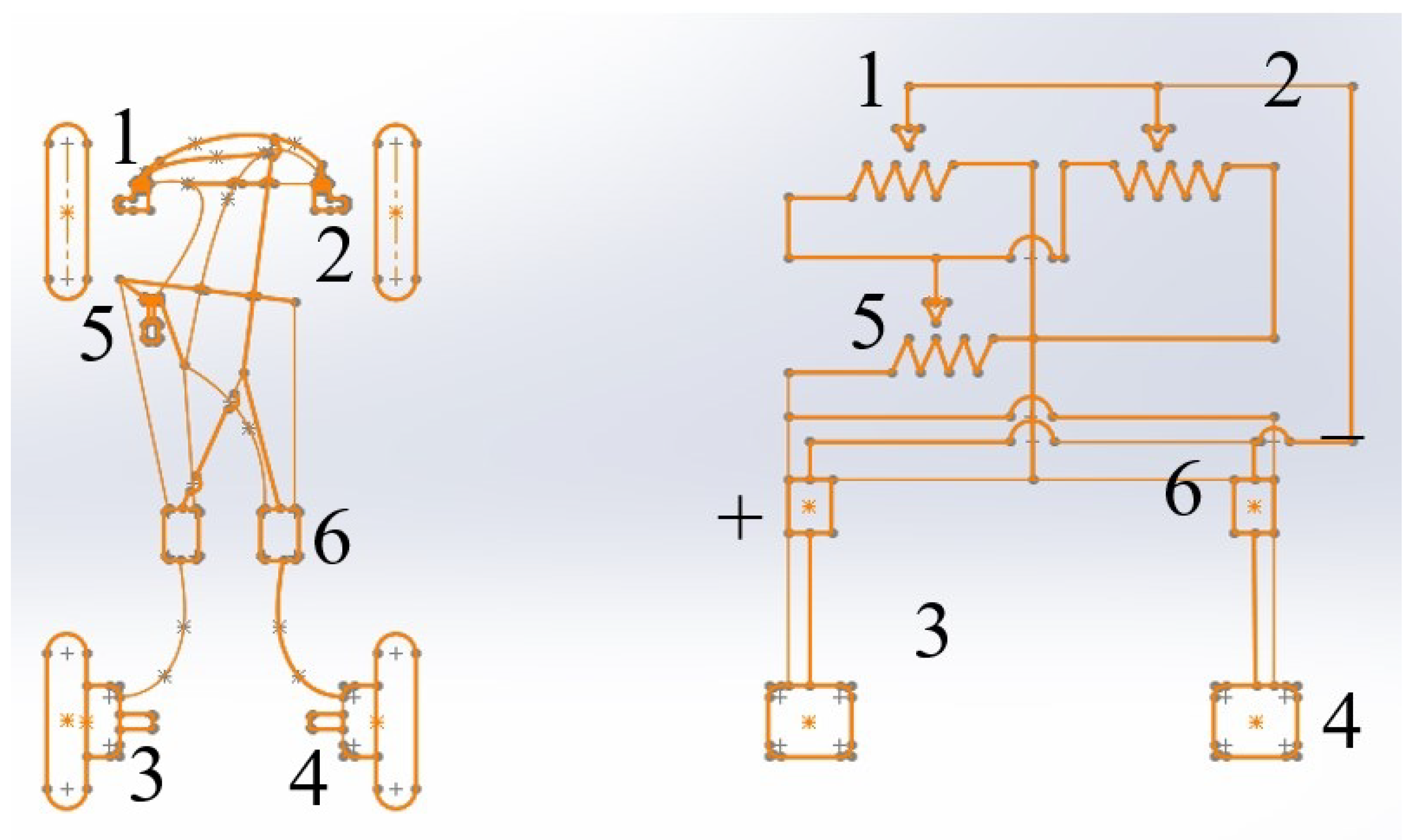
Consider an arrangement of two controllers, one for each HM engine on rims 3 and 4, and their respective throttle, but these need to be strategically placed between the chassis axles and the levers of the rotating masses of front rims 1 and 2.
These accelerators are connected in series to the main throttle control, which allows the vehicle to accelerate straight without the intervention of the accelerators of the mass, in this case, these accelerators must be completely closed to completely control main throttle 5 (Figure 9). When there is a curve, the accelerators act in series; that is, the accelerators connected to the mass lever, which connects to the SD, open at angle , causing the speed of HM4 to decrease, as per Equation (10). According to Equation (11), the accelerator connected to the mass lever should not be opened when in rectilinear mode, since this would mean a decrease in the speed of HM4 when turning right.
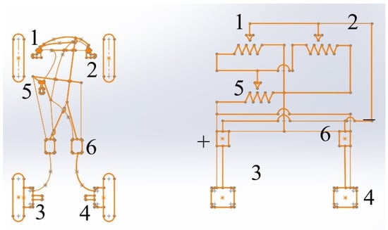
Figure 9.
DEM circuit diagram. On the left side are the location elements, while on the right side is the electrical circuit.
The percentage of opening of throttle hinge 1 is a function of Equation (11) (see Figure 9); in fact, the deceleration changes from 1 to ; that is,
where is the maximum opening of the hinge (see Figure 5). The previous equation can also be written as follows:
To determine the correct position that the accelerator should keep on the steering mass lever and its fixed counterpart on the chassis axis, the well-known accelerator hinge radius angle relationship is considered, which is .
Generally, the maximum angle of a commercial pedal accelerator is smaller than the maximum opening angle of the mass lever. Furthermore, according to Equation (11), the distance traveled by a fraction of the lever arm and must be the same as the opening of the accelerator; therefore,
And, substituting this into Equation (13), we obtain
Or, considering their respective approximation, Equations (11) and (12) can be equalized to obtain (), which are then substituted into (15) to obtain
The factor 1.27 could be reduced considering that, for small angles, the linearization .
4. Results
The electronic design of our DEM is based on Figure 6 and Figure 9. At , throttle 1 is completely closed; this is maximum acceleration mode. This throttle is connected on one side to controller 6 of HM4, and, on the other hand, it is connected in series to throttle 5, which has a complete knob to accelerate or decelerate, which allows a rectilinear advance.
For example, a right-hand turn of the inner rim causes throttle 1 to open (see Figure 12), allowing a decrease in the acceleration of rim 4 as a function of the angular ratio in Equation (10). Note that, in Figure 6, Figure 9 and Figure 12, accelerator 2 is not modified by this movement; therefore, accelerator 5 has direct control of HM3; and, according to Equation (10), the speed of HM4 depends on the speed of HM3 and the angle that relaxes accelerator 1.
Table 1 outlines the values for angle vs. factor speed f calculated with Equation (11); calculated with Equation (13) in cm; the of the theoretical HM4 calculated with Equation (10), which is graphed in Figure 10; and angle of the accelerator, which was calculated and converted to degrees. In order to carry out this scheme, consider a model of an urban EV with m and m; that is, , with an HM3 velocity of rpm, which is constant, an accelerator ratio cm, and a maximum throttle opening stroke cm.

Table 1.
Rotation angle with respect to ratio angular velocities f. Model 0.666.
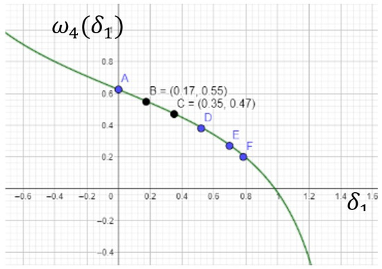
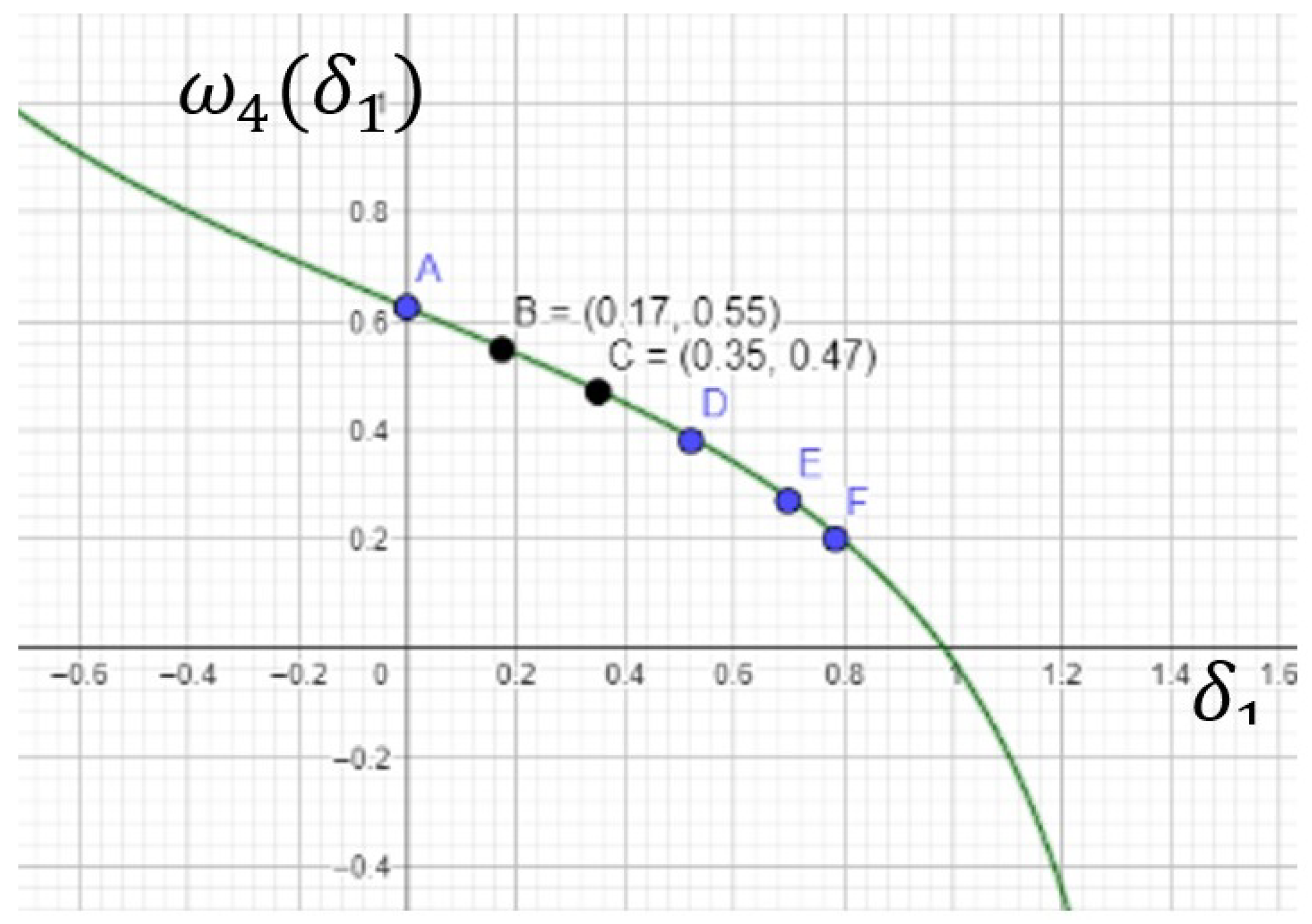
Figure 10.
Angular velocities (green) and (dots).
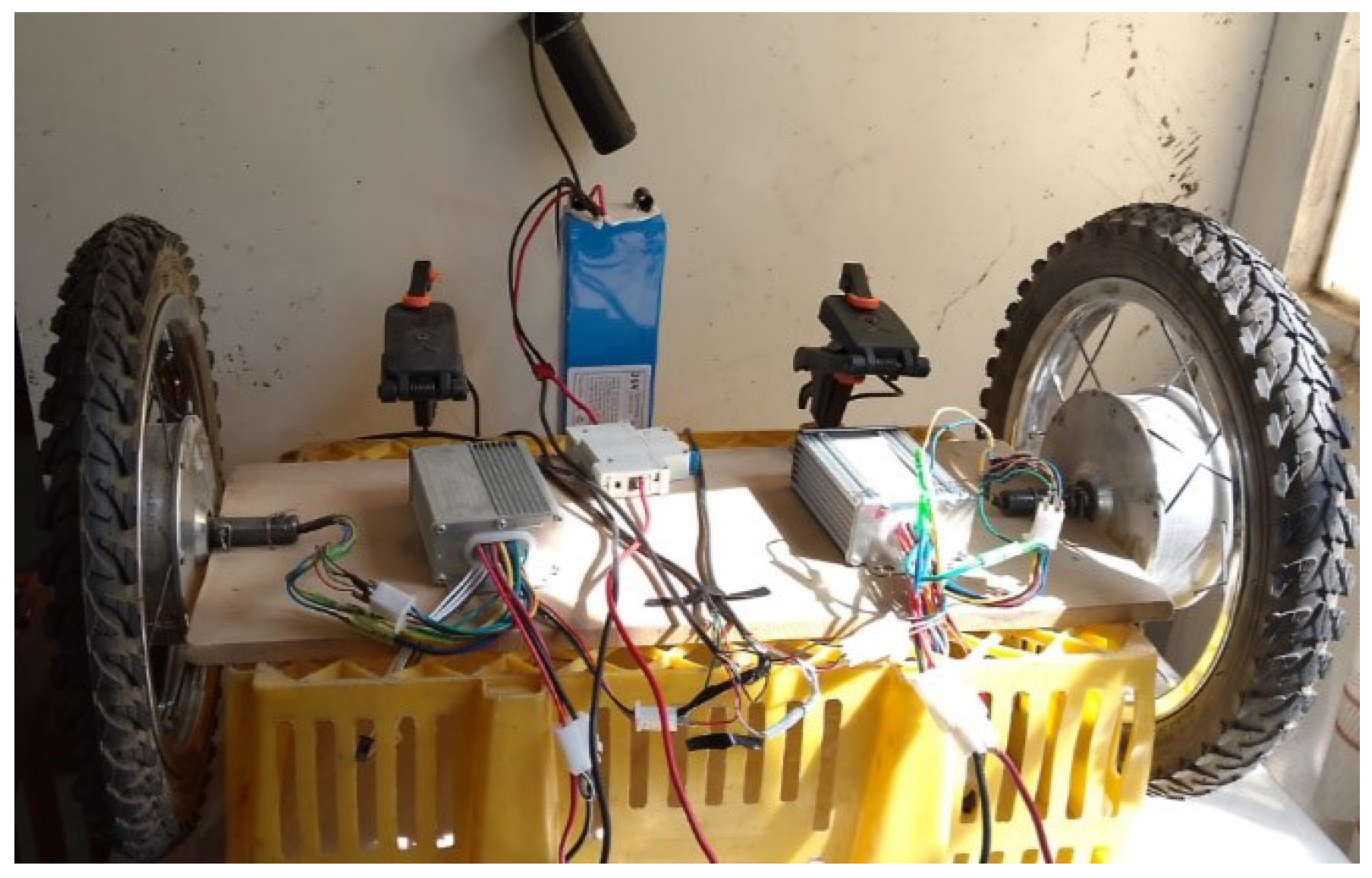
Table 2 presents the practical values obtained with the DEM prototype in Figure 11. The value of was obtained by pressing accelerator pedal 1 (see Figure 9) using the press shown in Figure 11, ensuring that the value was as close as possible to the values recorded in Table 1. Then, the lever arm was calculated using the following equation: . Finally, with the MQ4 operating at 625 rpm, the practical MQ4 speed, , was as dotted in Figure 10, which was measured with the prototype (see Figure 11).
Table 2.
Rotation angle with respect to angular velocity .

Figure 11.
DEM prototype for test simulation.
In the error analysis presented in Table 3, only the most representative values were considered to obtain , specifically, the three intermediate values.
Table 3.
Error table.
Analogous to how a prior author [7] related their theoretical results to their practical results, the same was performed here, maintaining the proportions in terms of the vehicle’s width and length. Although it is not exactly the same formulation, it can also be compared with Equation (10) as the same theoretical results for were achieved.
The results are analogous to those in [7,21] for an angle of with a speed of rpm (47.1 rad/s), where and , yielding a ratio of . This gives rpm (43.98 rad/s). Similarly, for an angle of , with a 10:1 scale, the results align with [7]. At a speed of rpm (22.5 rad/s), we obtain rpm (14.4 rad/s), as shown in Table 4.
Table 4.
Angle vs. factor f. Model 0.629.
Table 5 presents the practical values obtained from the DEM prototype shown in Figure 11 for DEM model 0.629, maintaining a constant speed of 215 rpm and subsequently of 450 rpm. The values of were closest to , and the speed of MQ4, denoted as in the prototype, was measured.
Table 5.
Angle vs. . Model 0.629.
The following graph presents the speed in Equation (10) as a function of in radians and vs. in radians.
The dots in the graph correspond to the speeds measured with the simulator; this is the prototype of the DEM, as shown in Figure 11, that was implemented in a small vehicle equipped with hub motors on the rear wheels. The vehicle operated with energy autonomy, utilizing solar panels and lithium batteries for power, as described in [8].
The press that holds the pedal accelerators simulated the compression of the steering levers. The hand accelerator simulated pedal accelerator 5, as shown in Figure 9. The left controller was programmed to make the motor operate in the opposite direction to the right motor, since the two were opposite to each other and thus both rotated in the same direction. For each point obtained in Table 2 for , the right accelerator was always kept depressed to allow all the control of the manual accelerator to almost achieve the maximum 625 rpm (this is extreme in the field), while the left pedal accelerator had openings in column with respect to angle . Similarly, two additional tests were conducted on this DEM prototype with constant speeds of 615 rpm and 450 rpm for wheel 3. The experimental data collected for wheel 4 are presented in Table 5.
Mechanism Design
According to Equation (16), the fraction of the lever to be considered for the placement of accelerator 1 is
With these data, it was possible to design the position of the pedal accelerator on the mass of the wheel and the chassis axle; that is to say that, a part of the pedal arm is fixed to the chassis axle, considering the end of the accelerator arm being fixed at 2.53 cm on the chassis axis. The other throttle arm connects to the ground rod that connects to the SD, as shown in the Figure 12. Note that this connection to the mass lever does not have an effect in the case of movement to the other side ; this movement must be disconnected since it would break the accelerator that is fixed to the chassis axis. This is the reason why the accelerator that is on the other tire of the vehicle (accelerator 2) does not participate when accelerator 1 opens.
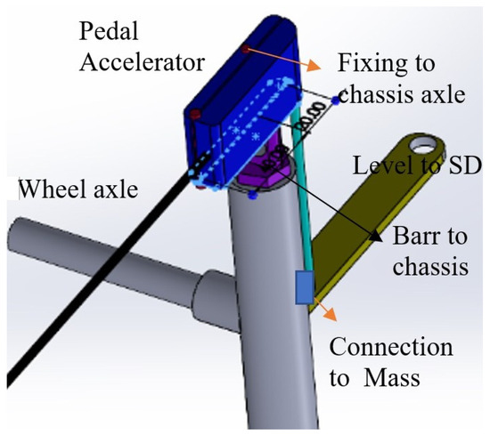
Figure 12.
Electric throttle fixed on chassis.
Figure 12 and Figure 13 represent two different schemes of differential accelerators. Figure 12 shows the details of how a part of the accelerator is fixed on the chassis axis and connected to the lever and mass of the tire, which connects to the SD; the hinge part is fixed on the chassis axis 2.5 cm from its end and 3.5 cm from the hinged end. This fixation is due to the fact that the throttle has a smaller opening than the opening of the SD lever arm. Furthermore, the analysis showed that the accelerator does not fully open; according to Table 1, it ranges from 0 to 2 cm. This is less than its maximum opening of 3 cm. On the other hand, the connection of the accelerator with the lever is flexible; that is, it is disconnected when it turns to the opposite side, according to Ackermann geometry. This disconnection is necessary, since it would otherwise break the accelerator that is fixed to the axis of the chassis.
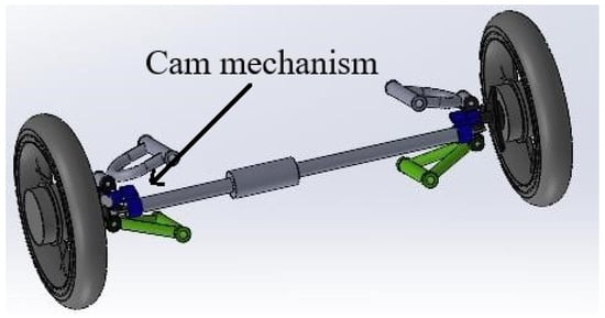
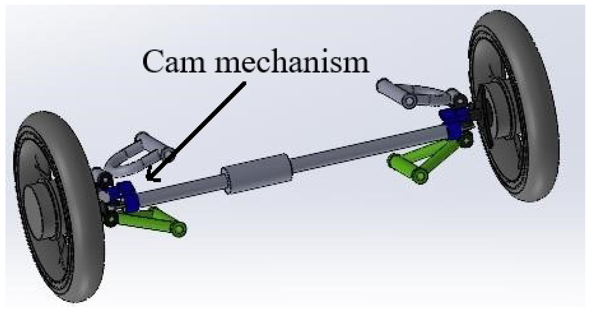
Figure 13.
Alternative design of accelerator of DEM on SD.
5. Conclusions
As demonstrated in this work, a DEM—constructed using a simple design based on three commercial pedal accelerators connected in a parallel-series configuration with their respective controllers—effectively functions as an electronic differential. The mechanical arrangement of the accelerators within the steering system replaces the need for electronic encoders, which are typically used for data collection ([3] and the references therein).
Figure 12 clearly illustrates the mechanism for opening the accelerator, which is connected to the controller, while Figure 13 presents different engineering approaches for designing drive devices according to various EV front-steering system configurations. In Figure 13, the action is controlled by a cam mechanism that allows the throttle to open only in one direction of rotation. Similarly, in Figure 12, the throttle opening is interrupted when rotation occurs in the opposite direction of the opening motion. In both cases, reverse action is not possible as turning in the opposite direction would force the accelerator to close, potentially causing damage.
The DEM prototype was implemented in a mini EV equipped with the same 350 W, 36 V motors, powered by 36 V Li-ion batteries and supplemented with solar panels for extended autonomy [8]. Additionally, Figure 12 considers the approximation . DEM model 1 was implemented, with the prototype being tested with DEM models 0.66 and 0.629.
One of the main drawbacks of the DEM system is that the commercial pedal accelerators are fragile as they are made of plastic. When screwed into the chassis mass and the steering linkage, they are prone to irreparable damage due to sudden movements. However, these accelerators can be manufactured using steel, which would allow them to withstand rough use.
Author Contributions
Conceptualization:A.J.R.B. and D.A.S.H.; methodology: A.J.R.B.; validation: A.J.R.B., Y.J.F., F.J.G.-R., A.M. and D.A.S.H.; formal analysis, A.J.R.B., F.J.G.-R. and D.A.S.H.; investigation, A.J.R.B., D.A.S.H. and Y.J.F.; resourcesL A.J.R.B.; data curation, A.J.R.B. and D.A.S.H.; writing—original draft preparation: D.A.S.H.; writing—review and editing: A.J.R.B., F.J.G.-R. and A.M.; visualization: A.J.R.B., F.J.G.-R. and D.A.S.H.; supervision: A.J.R.B.; project administration: A.J.R.B.; funding acquisition: A.J.R.B. and D.A.S.H. All authors have read and agreed to the published version of this manuscript.
Funding
This research received no external funding.
Institutional Review Board Statement
Not applicable.
Informed Consent Statement
Not applicable.
Data Availability Statement
The data presented in this study are available from the corresponding author upon request. The data are not publicly available as we do not have a publicly accessible repository.
Acknowledgments
The authors acknowledge A. Salas, M. Ramos, J. Clemente, A. Olgín, and M. Santillan for their help with the experimental work. A.J.R.B. acknowledges TECNM ITQ for support through a project on the integration of mechanical and solar energy in lithium batteries to contribute to the autonomy of electric vehicles.
Conflicts of Interest
The authors declare no conflicts of interest.
References
- Bandhauer, T.M.; Garimella, S.; Fuller, T.F. A Critical Review of Thermal Issues in Lithium-Ion Batteries. J. Electrochem. Soc. 2011, 158, R1. [Google Scholar] [CrossRef]
- Crouse, W.H. Transmisión y Caja de Cambios del Automóvil; McGraw-Hill: Barcelona, Spain, 1984; ISBN 9788426702289. [Google Scholar]
- Sharma, S.; Pegu, R.; Barman, P. Electronic Differential for Electric Vehicle with Single Wheel Reference. In Proceedings of the 2015 1st Conference on Power, Dielectric and Energy Management at NERIST (ICPDEN), Itanagar, India, 10–11 January 2015; pp. 1–5. [Google Scholar] [CrossRef]
- Hashemnia, N.; Asaei, B. Comparative Study of Using Different Electric Motors in the Electric Vehicles. In Proceedings of the 18th International Conference on Electrical Machines, Vilamoura, Portugal, 6–9 September 2008; pp. 1–5. [Google Scholar] [CrossRef]
- Deepak, K.; Frikha, M.A.; Benômar, Y.; Baghdadi, M.E.; Hegazy, O. In-Wheel Motor Drive Systems for Electric Vehicles: State of the Art, Challenges, and Future Trends. Energies 2023, 16, 3121. [Google Scholar] [CrossRef]
- Linares-Flores, J.; Castro-Heredia, O.; Garcia-Rodriguez, C. Diseño e Implementación de un Diferencial Electrónico para un Vehículo Eléctrico de Tracción de Cuatro Ruedas. 2022. Available online: http://repositorio.utm.mx:8080/jspui/handle/123456789/406 (accessed on 1 January 2022).
- Moazen, M.; Sharifian, M.B.B.; Sabahi, M. Electric Differential for an Electric Vehicle with 4WD/2WS Ability. In Proceedings of the 2016 24th Iranian Conference on Electrical Engineering (ICEE), Shiraz, Iran, 10–12 May 2016; pp. 751–756. [Google Scholar]
- Reséndiz Barrón, A.J.; Ramos Pérez, M.A.; Salas Flores, A.; García Rodriguez, F.J. Design and manufacture of electric vehicle body with solar panels for urban use. Rev. Cienc. Tecnol. 2025, 8, 1–14. [Google Scholar] [CrossRef]
- Contò, C.; Bianchi, N. E-Bike Motor Drive: A Review of Configurations and Capabilities. Energies 2013, 16, 160. [Google Scholar] [CrossRef]
- Kahveci, H.; Okumus, H.; Ekici, H. An Electronic Differential System Using Fuzzy Logic Speed Controlled In-Wheel Brushless DC Motors. In Proceedings of the 4th International Conference on Power Engineering, Energy and Electrical Drives, Istanbul, Turkey, 13–17 May 2013; pp. 881–885. [Google Scholar] [CrossRef]
- Haddoun, A.; Benbouzid, M.; Diallo, D.; Jamel, R.A.J.; Srairi, K. Design and Implementation of an Electric Differential for Traction Application. In Proceedings of the 2010 IEEE Vehicle Power and Propulsion Conference, Lille, France, 1–3 September 2010. [Google Scholar] [CrossRef]
- Tabbache, B.; Kheloui, A.; Benbouzid, M. An Adaptive Electric Differential for Electric Vehicles Motion Stabilization. IEEE Trans. Veh. Technol. 2022, 60, 104–110. [Google Scholar] [CrossRef]
- Chen, Y.; Wang, J. Design and Evaluation on Electric Differentials for Overactuated Electric Ground Vehicles with Four Independent In-Wheel Motors. IEEE Trans. Veh. Technol. 2012, 60, 1534–1542. [Google Scholar] [CrossRef]
- Tuncay, R.N.; Ustun, O.; Yilmaz, M.; Gokce, C.; Karakaya, U. Design and Implementation of an Electric Drive System for In-Wheel Motor Electric Vehicle Applications. In Proceedings of the 2011 IEEE Vehicle Power and Propulsion Conference, Chicago, IL, USA, 6–9 September 2011. [Google Scholar] [CrossRef]
- Magallán, G.A.; Bisheimer, D.A.H.G.; García, G.O. Implementación de un Diferencial Electrónico para Vehículos Eléctricos con un Único Controlador DSP. In Proceedings of the En las actas del Congreso [In XII Reunión de Trabajo en Procesamiento de la Información y Control], Córdoba, Spain, 16–18 October 2007; ISBN 9789871242238. [Google Scholar]
- Clavero-Ordóñez, L.; Fernández-Ramos, J.; Gago-Calderón, A. Electronic Differential System for Light Electric Vehicles with Two Inwheel Motors. In Proceedings of the International Conference on Renewable Energies and Power Quality (ICREPQ’18), Salamanca, Spain, 21–23 March 2018; pp. 326–329. [Google Scholar] [CrossRef]
- Aghili, F. Fault-Tolerant Torque Control of BLDC Motors. IEEE Trans. Power Electron. 2011, 26, 355–363. [Google Scholar] [CrossRef]
- Yıldırım, M.; Kurum, H. Electronic Differential System for an Electric Vehicle with Four In-Wheel PMSM. In Proceedings of the 2020 IEEE 91st Vehicular Technology Conference (VTC2020-Spring), Antwerp, Belgium, 25–28 May 2020. [Google Scholar] [CrossRef]
- Draou, A. Electronic Differential Speed Control for Two In-Wheels Motors Drive Vehicle. In Proceedings of the 4th International Conference on Power Engineering, Energy and Electrical Drives, Istanbul, Turkey, 13–17 May 2013; pp. 764–769. [Google Scholar]
- Perez-Pinal, F.J.; Cervantes, I.; Emadi, A. Stability of Electric Differential for Traction Applications. IEEE Trans. Veh. Technol. 2009, 58, 3224–3233. [Google Scholar] [CrossRef]
- Moazen, M.; Sabahi, M. Electric Differential for an Electric Vehicle with Four Independent Driven Motors and Four Wheels Steering Ability Using Improved Fictitious Master Synchronization Strategy. J. Oper. Autom. Power Eng. 2014, 2, 141–150. [Google Scholar]
- Yang, Y.P.; Xing, X.Y. Design of Electric Differential System for an Electric Vehicle with Dual Wheel Motors. In Proceedings of the 2008 47th IEEE Conference on Decision and Control, Cancun, Mexico, 9–11 December 2008; pp. 4414–4419. [Google Scholar] [CrossRef]
- Aggarwal, A. Electronic Differential in Electric Vehicle. Int. J. Sci. Eng. Res. 2013, 4, 1322–1330. [Google Scholar]
- Koladia, D. Mathematical Model to Design Rack and Pinion Ackerman Steering Geometry. Int. J. Sci. Eng. Res. 2014, 5, 716–720. [Google Scholar]

Disclaimer/Publisher’s Note: The statements, opinions and data contained in all publications are solely those of the individual author(s) and contributor(s) and not of MDPI and/or the editor(s). MDPI and/or the editor(s) disclaim responsibility for any injury to people or property resulting from any ideas, methods, instructions or products referred to in the content. |
© 2025 by the authors. Published by MDPI on behalf of the World Electric Vehicle Association. Licensee MDPI, Basel, Switzerland. This article is an open access article distributed under the terms and conditions of the Creative Commons Attribution (CC BY) license (https://creativecommons.org/licenses/by/4.0/).