Investigation of the Smoothness of an Intelligent Chassis in Electric Vehicles

Abstract

This study examines the smoothness of an intelligent chassis for electric vehicles, analyzes the chassis structure and configuration, and considers the impacts of the primary energy subsystem, electric drive subsystem, and auxiliary control subsystem on smoothness. The influence of suspension parameters on smoothness is examined, highlighting the significance of elastic element stiffness and the shock absorber damping ratio. Dynamic models of quarter- and half-car suspension systems, as well as a comprehensive nine-degree-of-freedom vehicle model, are developed to examine the vibration characteristics under varying road conditions. The chassis suspension dynamic model is developed, simulated, and analyzed using ADAMS/View software 2024. The suspension damping value is optimized with the ADAMS/PostProcessor tool, revealing that smoothness can be enhanced by judiciously decreasing the damping value. The article discusses the human body’s reaction to vibration and assessment metrics, referencing worldwide standards to establish a foundation for evaluation. The study offers theoretical backing for the design and optimization of an intelligent chassis, hence advancing the technological development of electric vehicles.

1. Introduction

Currently, individuals prioritize the smoothness and comfort of automotive operation to address these issues. This study examines the vehicle’s vibration characteristics and implements vibration control methods to increase passenger comfort and vehicle efficiency while adhering to performance criteria. This research is significant as it demonstrates that the human body acclimatizes to vibration frequencies experienced during walking that do not induce discomfort. Nevertheless, using an electric car results in a heightened frequency and amplitude of vibrations attributable to road conditions and chassis attributes. As smoothness diminishes, discomfort and cargo damage may ensue. The components of the vehicle may undergo wear and tear due to exposure to vibrations. The driver decreases the vehicle’s speed to facilitate a smooth journey on uneven terrain, hence diminishing transportation efficiency. Consequently, the examination of the smoothness of the electric vehicle’s smart chassis is crucial and appears to be essential.

Lei et al. used ADAMS software to improve the smoothness of the chassis for the wheel hub motor. It was discovered that the best chassis weight is 550 kg, which reduces peak vibration acceleration by 20% compared to the original design of 400 kg while greatly improving ride comfort [1]. Gu et al. delineate the concept and elucidate the attributes of modules within the automotive platform development paradigm and, in conjunction with the characteristics of automotive companies’ development platforms, investigate and analyze the evolution of modular chassis platforms for electric vehicles, proposing targeted recommendations and specific measures [2]. The intelligent control system for electric vehicle chassis developed by Yin et al. was tested using MATLAB/Simulink and Carsim simulation, which revealed that the system could significantly reduce the vehicle’s transverse swing angular velocity overshoot from more than 0.4 rad/s to close to 0.2 rad/s under the step input condition of the front wheel steering angle and reach the steady state in 0.5 s. Meanwhile, the technology efficiently reduces the center-of-mass lateral deflection angle from more than 0.06 rad to within 0.027 rad, considerably improving the vehicle’s handling stability and safety [3]. Cai et al. created an intelligent control system for electric vehicle chassis that was tested using MATLAB/Simulink and Carsim simulation, demonstrating that the system could effectively regulate the vehicle’s dynamic response under front wheel steering angle step input conditions. The simulation experimental conditions are established as the driver spins the steering wheel to 80° in 0.3 s, keeps the initial speed at 80 km/h, and the road surface adhesion coefficient is set at 0.85, while the quantization factor k1 = 50 and scaling factor k2 = 3000 are applied simultaneously. The simulation shows that the system provides a good real-time control response, which considerably improves the vehicle’s maneuvering stability and safety [4]. Y.W. Hu et al. optimized a light electric car chassis using ADAMS software. The results reveal that by adjusting the chassis weight from 400 kg to 550 kg, the force on the passengers when crossing an obstruction is lowered from 268 N to 84 N. The redesigned chassis greatly increases riding comfort and vehicle stability [5].

Mirzaeinejad H. et al. validated their integrated vehicle active steering and differential braking control system with simulation studies. Under the steering angle step input situation, the system considerably decreases the vehicle’s traverse angular velocity overshoot while also controlling the traverse angular velocity tracking error within a short range. At the same time, the vehicle’s center-of-mass lateral deflection is effectively limited to 0.027 rad, resulting in significantly improved directional stability and maneuverability. Furthermore, the system optimizes the control strategy to reduce the vehicle’s longitudinal speed reduction by approximately 30% when compared to the individual braking control strategy [6]. Rengaraj et al.’s integrated chassis control system improved high-speed cornering stability by significantly reducing the traverse angular velocity and side deflection angle under two-lane change conditions, as demonstrated by the MATLAB/Simulink simulation. Specifically, the integrated control strategy reduces the traverse angular velocity by about 50% and controls the side deflection angle within 0.027 rad, which exhibits better handling performance compared to the individual control strategies and significantly improves the stability and safety of the vehicle on both high- and low-friction surfaces [7]. The optimal design methodology for a high-performance automotive chassis developed by Cavazzuti et al. [8] through the use of topology optimization, shape optimization, and dimensional optimization in a cascade approach showed that the method was able to significantly reduce the chassis weight while meeting the performance constraints of structural stiffness, modal response, and crash behavior. Compared with the Ferrari F458 Italia chassis, the weight of the optimized chassis is reduced by about 20%. Meanwhile, the optimization process ensures that the chassis meets the design requirements in terms of global bending stiffness, torsional stiffness, and local stiffness through reasonable constraint settings and parameter adjustments, which significantly improves the structural performance and lightweight level of the chassis. Sharmila et al. created an electric vehicle model that was validated using a MATLAB/Simscape simulation and demonstrated that the model can greatly enhance vehicle performance over a wide range of driving cycle circumstances. The conditions can greatly improve vehicle performance. A PI controller optimizes the motor and vehicle speeds, causing the vehicle speed to almost exactly follow the reference curve, with a very small deviation from the reference speed. At the same time, the model effectively recovers energy using regenerative braking technology, which significantly increases the battery range and keeps the battery’s state of charge (SoC) high. These findings suggest that the electric vehicle concept offers notable benefits in terms of performance, environmental friendliness, and energy efficiency [9]. A heavy-duty vehicle chassis was built, examined, and optimized by Abdulkadir Yasar et al. using the Taguchi method and Finite Element Analysis (FEA). According to the study’s findings, the overall deformation of the chassis is considerably decreased when the A1B2C1D1 chassis design, which uses AISI 1006 steel, a 6 × 4 wheel pattern, a U-section, and an unsupported chassis design, is combined. The overall deformation of this design combination is reduced to 4.1864 mm and 6.1516 mm, respectively, under loads of 100 kN and 150 kN, which is noticeably better than the other design combinations. This suggests that the optimized design offers a practical solution for the lightweight and high-performance design of heavy vehicle chassis, as well as notable benefits in enhancing the structural performance and deformation resistance of the chassis [10].

The goal of this study is to look into the smoothness of an electric vehicle’s smart chassis and adjust the suspension characteristics to improve ride comfort and safety. This study not only confirms the model’s validity but also establishes the best range of suspension damping ratios to improve vehicle smoothness by building an accurate dynamic model and performing a simulation analysis using ADAMS software. The study’s findings have important implications for the design of electric vehicle chassis, providing a solid theoretical foundation and practical direction for improving future electric vehicle performance and ride quality.

Furthermore, this study’s academic contribution and practical application value stem from its ability to provide fresh ideas and solutions for technical growth in the field of electric vehicles. By optimizing the suspension system, not only can the vehicle’s dynamic performance be enhanced but the marketization of electric vehicles may also be facilitated in order to fulfill rising customer demand for comfort and safety. This study also identifies potential future research directions, such as more comprehensive parametric considerations and validation in real vehicle tests, which will strengthen the scientific and practical aspects of the study’s findings and contribute to the long-term development of the electric vehicle industry.

2. Intelligent Chassis Structure and Configuration for Electric Vehicles

2.1. Examination of the Intelligent Chassis Structure and Configuration of Electric Vehicles

2.1.1. Primary Energy Subsystems

The control system, power supply, and charging device can constitute an energy system. The electric vehicle energy management system includes a conversion device primarily utilized for energy management, with many types available for selection. The motor provides the energy necessary for the car’s operation, ensuring both the vehicle’s functionality and the appropriate operation of its many pieces of equipment.

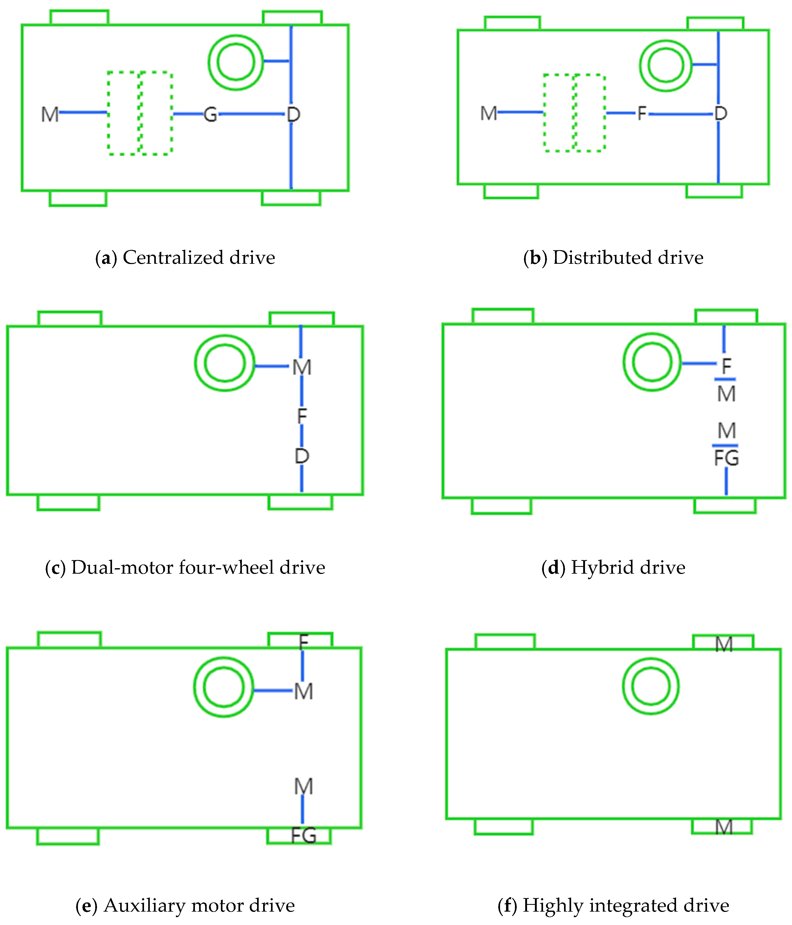
2.1.2. Power Drive Subsystems

The electronic control unit, electric motor, converter, and drive wheels are essential components of the propulsion system. Figure 1 illustrates various configurations of the drive subsystem on the chassis of an electric vehicle.

Figure 1 depicts six distinct drive system configurations, each tailored to a specific application and performance requirement. Among them, (a) centralized drive uses a single electric motor to send power to the wheels through a driveshaft, which is a basic and low-cost structure suited for cost-sensitive cars that do not require great power distribution but have high energy loss and restricted dynamic performance. (b) Distributed drive supplies each wheel or set of wheels with a separate electric motor, allowing for a flexible power distribution and greatly improving vehicle dynamics and maneuverability, making it suited for high-performance and self-driving cars. (c) Dual-motor four-wheel drive employs electric motors at the front and back of the vehicle to drive the front and rear wheels, respectively, to provide higher grip and passing power, and is appropriate for challenging road conditions, such as off-road vehicles or high-performance SUVs. (d) Hybrid drive combines an electric drive and a conventional fuel-driven drive, where the electric motor and the internal combustion engine can be switched or work in tandem depending on the operating conditions, which improves fuel economy and reduces emissions while maintaining the range of a conventional fuel-driven vehicle and is suitable for a combination of urban and long-distance driving needs. (e) The auxiliary electric motor drive is mostly used to offer additional power support when the vehicle is beginning or accelerating in order to increase acceleration performance and reduce the energy consumption of the primary drive system. (f) In highly integrated drive, electric motors, transmissions, controllers, and other components are highly integrated to form a compact power unit, significantly reducing the system’s weight and volume, improving space utilization and system efficiency, and making it suitable for vehicles with high space and efficiency requirements. These configurations provide diversified choices for the design and development of electric vehicles and can meet the needs of different users and application scenarios, thus realizing the best balance of performance and efficiency.

The powertrain of a vehicle is driven by an electric motor. While series-excited DC motors were once used in electric vehicles, permanent magnet synchronous motors (PMSMs) and AC induction motors are now preferred for their high efficiency and reliability. These motor technologies help reduce weight, size, and energy consumption and improve NVH performance (noise, vibration, and acoustic roughness). Consequently, advanced mechanical components are essential for chassis components [11]. BYD has produced the world’s inaugural series all-electric assembly, including an eight-in-one motor. The assembly comprises an electric motor, a gearbox, an electric drive controller, a DC-DC converter, a 12 V on-board charger (OBC), a power distribution unit (PDU), a battery management system (BMS), and an on-board control unit (VCU). The system features a highly integrated array of functional modules aimed at optimizing space use and minimizing weight, distinguished by its high integration, power density, and efficiency. To further diminish energy usage, the four-wheel-drive architecture featuring two motors at both the front and rear can substantially enhance the vehicle’s acceleration. To achieve stable performance at medium and high speeds, a single engine can fulfill the power demands of the entire vehicle. Conventional permanent magnet synchronous motors operate with more efficiency than asynchronous motors. During no-load rotation, the magnetoresistive losses in permanent magnet synchronous motors (PMSMs) markedly escalate, leading to increased energy consumption during high-speed operation. For the first time, the vehicle utilizes an innovative power compound structure comprising permanent magnet synchronous and combined asynchronous motors. During acceleration, both motors operate concurrently; when the asynchronous motors are deactivated and only the permanent magnet synchronous motors function, the stable driving conditions yield all-wheel-drive performance akin to that of a two-wheel-drive, along with optimized energy consumption.

The drive function of an electric car is to transmit engine drive torque to the vehicle’s driveshaft, and the majority of the drive components are often compact when utilizing electric drive. As the electric motor may initiate operation under load, it is unnecessary to correlate traditional fuel vehicles with electric vehicles. The drive motor’s rotational direction can be altered via a chain, eliminating the necessity to reverse an electric car in an internal combustion engine powertrain. Contemporary electric vehicles represent a significant departure from traditional gasoline vehicle transmissions, omitting certain components.

2.1.3. Auxiliary Control Subsystems

The auxiliary control subsystem is responsible for power steering, temperature regulation, and an auxiliary power supply. The auxiliary power supply system delivers various voltage levels and the necessary power for the electric vehicle’s auxiliary system. It primarily provides power for steering, air conditioning, braking, and more accessories. The electric vehicle speed control system is engineered to modify the velocity and orientation of the electric vehicle. Historically, speed control was typically achieved using series resistance and several other means. Stepper speed control is hardly employed today because of its intricate construction and increased energy usage. Thyristor speed control is presently prevalent in electric vehicles due to its advancement over prior speed control methods and its effective implementation of stepless speed regulation. In drive motor switching control, DC motors utilize contactors to alter the armature current or magnetic field direction for speed modulation. This complicates the circuit and diminishes reliability. Simultaneously simplifying the circuit and altering the phase sequence facilitates the reversal of the AC asynchronous motor’s direction, a method that enhances energy recovery and simplifies control.

The steering wheel, steering gear, and additional components constitute the steering system, which facilitates vehicle maneuvering during transit. When we exert a steering force on the steering wheel, the force is conveyed downward, causing a shift that alters the direction. Currently, steering mechanisms, including mechanical, hydraulic, and electric power steering, can be classified into three categories based on the following principle: when the driver exerts torque on the steering wheel in an attempt to rotate it, the torque sensor transforms the cornering signal into an electrical signal and transmits it to the control unit, along with the speed data. Utilizing these signal inputs, the control unit computes the output torque and engine orientation, thus generating a signal. The output signal regulates the electric motor via a circuit.

2.2. Examination of Suspension Effects on Chassis Structure Smoothness

2.2.1. Human Reaction to Vibration and Assessment Metrics of Vehicle Smoothness

The examination of smoothness entails analyzing vibration findings to regulate the amplitude within specified assessment criteria, ensuring that it does not go beyond the standard range; otherwise, smoothness will diminish. Various standards exist for assessing the smoothness of a car body, with the Janeway grading model being the most prevalent due to its extensive ratings and criteria for numerous components of the automobile body.

Subjective evaluations are conducted due to the unique physiological variations across individuals, resulting in diverse reactions to vibration. An objective evaluation of vehicle design considers elements such as the vibration frequency and intensity, alongside human acceptance tests, to determine the levels of vibration that are acceptable to the majority of individuals.

After studying numerous vibration cases, a model was developed to evaluate the effect of driver position on human vibration. The model primarily utilizes the seat as a reference for the analysis of linear and angular vibrations. The simulation of linear and axial vibrations of a human seat is investigated in this context [8]. Figure 2 [12] illustrates the human seated vibration model, depicting 12 axial vibrations.

Table 1. Relationship between weighted acceleration rms and humans’ subjective feelings, adapted from Ref. [13].

$\mathbf{Weighted} \mathbf{Acceleration} \mathbf{RMS}/(\mathbf{M}/{\mathbf{S}}^2$)	Subjective Perception of the Human Body
<0.315	It is not uncomfortable.
0.315~0.63	Slightly uncomfortable
0.5~1.0	Feel ill
0.8~1.6	Uncomfortable
1.25~2.5	It is very uncomfortable.
>2.0	Dreadfully uncomfortable

[12] illustrates the correlation between discomfort levels and the root-mean-square value of weighted vibration acceleration. The body region most responsive to vibration frequencies is between 4 and 12.5 Hz. The body’s internal organs can tolerate frequencies of 4 to 8 Hz, whereas frequencies over 8 Hz impact the spine.

Vehicle smoothness is mainly assessed by human perception, requiring an analysis of vibrations’ impacts on the body and ensuring proper functionality and driving posture. Research shows that the optimal smoothness is achieved when the chassis vibration frequency matches that of a walking person (1–1.6 Hz), with a vibration acceleration limit of 0.2–0.3 g. To prevent load damage and ensure safety, vibration acceleration must stay below 0.6 g, as exceeding 1 g can cause unsecured loads to detach, posing significant risks [14].

2.2.2. Impacts of Vehicle Suspension Parameters on Ride Smoothness

The car suspension serves as a link between the frame and the tires, primarily to mitigate the discomfort given to people by road surface irregularities and to protect cargo from damage due to vibrations. The suspension constitutes merely a component of the chassis, which is comprised of multiple elements, and the selection of its settings directly influences the vehicle’s smoothness.

Elastic components, in conjunction with shock absorbers and guides, constitute the suspension system of a vehicle. The elastic components serve to link the vehicle to uneven terrain, reducing vibrations and safeguarding occupants and cargo from such disturbances. The shock absorber in the suspension is designed to convert the car’s vibrations to mitigate its oscillations. The rail mechanism in the suspension functions as a force transmission system and is essential for all types of suspension.

The elastic component in the suspension possesses a stiffness value, which denotes the alteration in the suspension due to the applied force, typically expressed by its frequency, while the bias frequency n commonly signifies the frequency generated by its free oscillation. A lower bias frequency n enhances the vehicle’s smoothness and reduces body vibrations perceived by the driver [15]. Currently, the values of the characteristic parameters for various automobile components are defined to enhance performance, with the front suspension’s bias frequency specified between 1 and 1.3 Hz and the rear suspension generally specified between 1.2 and 1.5 Hz.

The standard correlation among the bias frequency $\mathrm{n}$, spring stiffness$c$, and spring mass $m$ is [16]

$$\mathrm{n}={\displaystyle \frac{1}{2\mathsf{\pi }}}\sqrt{{\displaystyle \frac{c}{m}}}$$

(1)

In Equation (1), $\mathrm{n}$ represents the bias frequency in Hz, $c$ denotes the stiffness in N/mm, and $m$ signifies the mass of the spring load in t.

To enhance the smoothness of a vehicle with a specific spring load mass, the stiffness of the elastic element (spring) must be reduced to decrease its frequency deviation. The reduced rigidity of the elastic element amplifies its deformation, resulting in heightened stress and potential damage to the element. The substantial deflection is constrained by the available space, hence restricting the whole travel of the suspension. The aggregate of static and dynamic deflections must not exceed 160 mm, with dynamic deflections typically constrained to a range of 1/2 to 2/3, accounting for the compression of the block.

If a car’s suspension lacks any damping components and contains only a central spring, the spring will continue to oscillate until it exhausts its energy, resulting in significant instability. This underscores the necessity of incorporating a shock absorber into the suspension system.

A comprehensive analysis of the experimental data revealed that the vertical acceleration of body vibration is comparatively minimal when traversing well-maintained roadways. To guarantee optimal driving comfort, the suspension attenuation coefficient must be calibrated to 0.1748; under poor road conditions, the vertical acceleration of vibrations is significantly elevated. For optimal driving safety, the damping ratio must be established at 0.4136 when the suspension damping ratio is optimized for safety; under mild road conditions, the ideal damping ratio should be defined in the range of [0.1748, 0.4136].

Figure 3 [16] illustrates that the ratio of the body vibration acceleration curve to the attenuation coefficient reveals an attenuation ratio of [0.1748, 0.4136], with the body vibration acceleration being minimal. Consequently, the damping ratio of the shock absorber must be calibrated within this range.

F represents the recovery resistance of the automotive damper, which is computed as follows [16]:

$$F=kv$$

(2)

In Equation (2), F is the recovery resistance of the damper in N; k is the damping coefficient of the damper in Ns/m; and v is the velocity in m/s.

The damping ratio of the damper is calculated as follows [16]:

$$\zeta ={\displaystyle \frac{k}{2\sqrt{cm}}}$$

(3)

In Equation (3) $\zeta$ is the damping ratio; k is the damping coefficient of the damper in Ns/m; c is the stiffness of the elastic element (spring) in N/m; and m is the mass of the spring load in kg.

Equation (3) illustrates that the damping ratio of a shock absorber is correlated with its damping coefficient, spring stiffness, and suspension mass. Extensive investigation reveals numerous combinations of stiffness and spring mass values in the suspension, each yielding distinct effects that can be chosen based on the required damping. An overview of scientific data has been compiled into

Table 2. Optimal damping ratios for automotive suspensions according to surface smoothness.

Vehicle Type	Suspensions	Damping Ratio
Enclosed Carriage	front suspension	0.4
	rear suspension	0.2
Lorry	front suspension	0.4
	rear suspension	0.3

[12], which includes several classic damping ratios.

The classification as a sprung or unsprung mass is contingent upon the presence of springs. Unsprung masses, commonly referred to as unsuspended masses, include components such as axles, tires, and rims. Spring-loaded masses should be minimized in size. They are calibrated to 18–22% to optimize their performance.

3. Research on the Vibration Theory Modeling of Electric Vehicle Intelligent Chassis

3.1. Vibration Analysis of One-Quarter Vehicle Suspension Systems

3.1.1. Simplification of the Complete Vehicle Model

During experimental operations, we face intricate vibration systems, as increasingly complicated models closely resemble real situations, hence enhancing the realism and accuracy of the entire simulation experiment. Nevertheless, this frequently renders the analysis exceedingly burdensome. Consequently, when modeling the mechanics of a vibrating system, we consistently simplify it in terms of representation and reality. The seven-degree-of-freedom automobile model encompasses three degrees of freedom—vertical, tilt, and roll—in addition to four vertical degrees of freedom for the four-wheel drive system. The wheels and axles constitute the unsprung mass, whereas the body, along with other components like the frame, comprise the oversprung mass utilized for attachment [17]. Assume that the product of the distances from the origin to the front and rear suspensions, together with the square generated by rotating the body about the Y-axis, are highly analogous, while both exhibit distinct vertical vibrations simultaneously. Subsequently, we can further simplify the model to derive a vibration model, as illustrated in Figure 4 [18].

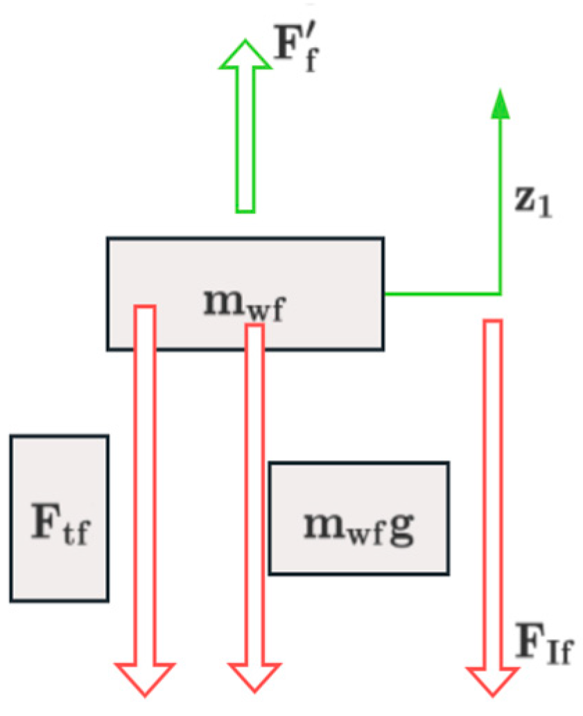
3.1.2. Mathematical Modeling of a Two-Mass Vibration System

The vibration model of the two-mass system may represent both the dynamic properties of the body components and those of the wheel components within the high-frequency resonance range of 10 Hz to 15 Hz. Thus, we can designate the vertical displacement coordinates at the midpoint between the wheel and the body. Identify the coordinate origin at the corresponding equilibrium location and formulate the differential equations [18] for the aforementioned single-wheel dual-degree-of-freedom dual-mass model:

$$\begin{gathered} m_2{\ddot{z}}_2+c\left({\dot{z}}_2 - {\dot{z}}_1\right)+k\left(z_2 - z_1\right)=0 \\ {m}_1{\ddot{z}}_1+c\left({\dot{z}}_1 - {\dot{z}}_2\right)+k\left(z_1 - z_2\right)+k_t\left(z_1 - q\right)=0 \end{gathered}$$

(4)

where $m_2$ is the suspension mass (on-spring mass, including the body, etc.); $m_1$ is the non-suspension mass; k and $k_t$ are the suspension and tire stiffnesses, respectively; and c is the suspension damping coefficient. Where the force analysis is performed on $m_1$, the suspension spring force is $F_{k1}=k_1\left(z_2-z_1\right)$ and the suspension damping force is $F_c=c\left({\dot{z}}_2-{\dot{z}}_1\right)$. For the force analysis on $m_2$, the suspension reaction force is $-k_1\left(z_2-z_1\right)-c\left({\dot{z}}_2-{\dot{z}}_1\right)$, and the tire spring force is $k_2\left(z_0-z_2\right)$.

Second-order differential equations in matrix form define the displacement vector $z={\left[\begin{array}{c}{z}_1,z_2\end{array}\right]}^{\top }$, and the system equation can be expressed as

$$M\ddot{z}+C\dot{z}+Kz=F\left(t\right)$$

(5)

Among them, $M=\left[\begin{array}{cc}{m}_1& 0\\ 0& m_2\end{array}\right],C=\left[\begin{array}{cc}c& -c\\ -c& c\end{array}\right]$,

$$K=\left[\begin{array}{cc}{k}_1& -k_1\\ -k_1& k_1+k_2\end{array}\right], F\left(t\right)=\left[\begin{array}{c}0\\ k_2{z}_0\left(t\right)\end{array}\right]$$

State variables are defined for the purpose of controller design and numerical simulation:

$$x={\left[z_1,{\dot{z}}_1,z_2,{\dot{z}}_2\right]}^{\top }, u=z_0\left(t\right)$$

(6)

The system equations are converted to state space form:

$$\dot{x}=Ax+Bu$$

(7)

Among them,

$$A=\left[\begin{array}{cccc}0& 1& 0& 0\\ -{\displaystyle \frac{k_1}{m_1}}& -{\displaystyle \frac{c}{m_1}}& {\displaystyle \frac{k_1}{m_1}}& {\displaystyle \frac{c}{m_1}}\\ 0& 0& 0& 1\\ {\displaystyle \frac{k_1}{m_2}}& {\displaystyle \frac{c}{m_2}}& -{\displaystyle \frac{k_1+k_2}{m_2}}& -{\displaystyle \frac{c}{m_2}}\end{array}\right], B=\left[\begin{array}{c}0\\ 0\\ 0\\ {\displaystyle \frac{k_2}{m_2}}\end{array}\right]$$

If the system is not damped, the body and wheels each vibrate freely without damping at their respective intrinsic frequencies of displacement frequency; $p_0=\sqrt{k/m_2}$ and $p_t=\sqrt{\left(k+k_t\right)/m_1}$ are two of the intrinsic frequencies, which have not been considered as damped and are used as part of the mass vibration. In the unshocked free vibration, the body mass and wheel mass are at the same circular frequency ω and phase angle $\phi$ for simple harmonic vibration, and the wheel and body amplitudes are set to be $z_{10}$ and $z_{20}$, respectively; then, their vibration responses are [18]

$$\begin{gathered} z_1=z_{{10}^{e^{j(\omega t+\phi )}}} \\ {z}_2=z_{{20}^{e^{j(\omega t+\phi )}}} \end{gathered}$$

(8)

The system frequency response function can be expressed as follows:

$$H\left(\omega \right)={\left(-{\omega }^{2}M+j\omega C+K\right)}^{-1}{F}_0$$

(9)

where $F_0={\left[0,k_2{Z}_0\right]}^{\top }$ can be evaluated by analyzing the amplitude–frequency characteristic curves to assess the influence of the suspension parameters on the vibration attenuation.

By setting the damping c to zero and substituting the above set of equations into Equation (4), then substituting $p_0$ and $p_t$ and simplifying gives [18]

$$\begin{gathered} \left({p_0}^2 - {\omega }^2\right)z_{20} - {p_0}^2{z}_{10}=0 \\ -{\displaystyle \frac{k}{m_1}}{z}_{20}+\left(p_{t_2} - {\omega }_2\right)z_{10}=0 \end{gathered}$$

(10)

The two roots in Equation (10) are the squares of the sum of the two principal frequencies of the two-degree-of-freedom system. So, the first-order and second-order principal vibration patterns are sufficient to find [18] the first-order principal vibration pattern

$${\left({\displaystyle \frac{z_{10}}{z_{20}}}\right)}_1={\displaystyle \frac{{p_0}^2 - {{\omega }_1}^2}{{p_0}^2}}$$

(11)

and the second-order principal vibration mode

$${\left({\displaystyle \frac{z_{10}}{z_{20}}}\right)}_2={\displaystyle \frac{{p_0}^2 - {{\omega }_2}^2}{{p_0}^2}}$$

(12)

3.2. Dynamics of a One-Half Vehicle Suspension System

Figure 5 [19] illustrates the one-half vehicle suspension system model.

Here, e$m_c$ is one-half of the body mass; $I_c$ is one-half of the body moment of inertia; ${\theta }_c$ is the pitch angle at the center of mass of the body; $z_c$ is the vertical displacement of the center of mass; $z_2,z_4$ is the vertical displacement of the front and rear bodies; a, b is the distance from the center of mass of the body to the front and rear axles; L is the axle distance, and L = a + b; $m_{wf},m_{wr}$ is the unsprung mass of the front and rear wheels; $k_{tf},k_{tr}$ is the stiffness of the front and rear tires; $z_{0f},z_{0r}$ is the vertical displacement of the ground of the front and rear wheels; $k_{sf},k_{sr}$ is the stiffness of the damping springs of the front and rear suspensions; and $c_{sf},c_{sr}$ is the vertical displacement of the front and rear tires. $z_1,z_3$ is the damping coefficient of the front and rear suspension.

Since the front and rear wheels are traveling in the same lane, the road inputs $Z_{0f}$, $Z_{0r}$ for the front and rear wheels differ by only one time lag $\mathsf{\Delta }t$ [19]:

$$\mathsf{\Delta }t=L/u$$

(13)

where $u$ is the vehicle speed.

Use the position of the spring when it is not deformed as the origin of the equations that create the dynamics of the system. The forces acting on the upper part of the body are shown in Figure 6, and the equilibrium equations are as follows [19]:

$$F_f+m_{c}g+F_I+F_r=0$$

(14)

$$I_c{\ddot{\theta }}_c - a{F}_f+b{F}_r=0$$

(15)

where $F_f$ is the front suspension force, $F_f=K_{sf}\left(z_2-z_1\right)+C_{sf}\left({\dot{z}}_2-{\dot{z}}_1\right)$; $F_r$ is the rear suspension force, $F_r=K_{sr}\left(z_4-z_3\right)+C_{sr}\left({\dot{z}}_4-{\dot{z}}_3\right)$; and $F_I$ is the center of mass inertia force, $F_I=m_c{\ddot{z}}_c$.

To organize Equations (14) and (15), substitute the formulas of $F_f$, $F_r$, and $F_I$ to obtain the following formulas [19]:

$$m_c{\ddot{z}}_c=- K_{sf}\left(z_2 - z_1\right) - C_{sf}\left({\dot{z}}_2 - {\dot{z}}_1\right) - K_{sr}\left(z_4 - z_3\right) - C_{sr}\left({\dot{z}}_4 - {\dot{z}}_3\right) - m_{c}g$$

(16)

$$I_c{\ddot{\theta }}_c=a{K}_{sf}\left(z_2 - z_1\right)+a{C}_{sf}\left({\dot{z}}_2 - {\dot{z}}_1\right) - b{K}_{sr}\left(z_4 - z_3\right) - b{C}_{sr}\left({\dot{z}}_4 - {\dot{z}}_3\right)$$

(17)

The force analysis [19] of the front wheel is shown in Figure 7, and the equilibrium equation is as follows [19]:

$$F_{tf}+m_{wf}g+F_{If}+F_f^{\prime }=0$$

(18)

where $F_{tf}$ is the front wheel vertical force; $F_{If}$ is the front wheel inertia force, $F_{If}=m_{wf}{\ddot{z}}_1$; and $F_f^{\prime }$ is the front suspension force, $F_f^{\prime }=-F_f$.

When organizing Equation (18), the following formula is obtained by substituting the formulas of $F_f$, $F_{If}$, and $F_f^{\prime }$ [19]:

$$m_{wf}{\ddot{z}}_1=- {F\dots .}_{tf}+K_{sf}\left(z_2 - z_1\right)+C_{sf}\left({\dot{z}}_2 - {\dot{z}}_1\right) - m_{wf}g$$

(19)

The equations of motion for the rear wheels can be calculated in the same way as above to give the following equation [19]:

$$m_{wr}{\ddot{z}}_3=- F_{tr}+K_{sr}\left(z_4 - z_3\right)+C_{sr}\left({\dot{z}}_4 - {\dot{z}}_3\right) - m_{wr}g$$

(20)

The value of $F_{tf}$ is specified here as follows [19]:

$$F_{tf}=\left\{\begin{array}{ll}0& z_1\ge z_{0f}\\ K_{tf}\left(z_1-z_{0f}\right)& z_1<z_{0f}\end{array}\right.$$

(21)

The rear wheel vertical force $F_{tr}$ also complies with this.

So, the one-half vehicle suspension dynamic equations are given as follows [19] when the tires are off the ground ($z_1\ge z_{0f},z_3\ge z_{0r}$):

$$\left\{\begin{array}{c}{m}_c{\ddot{z}}_c=-K_{sf}\left(z_2 - z_1\right)-C_{sf}\left({\dot{z}}_2 - {\dot{z}}_1\right)-K_{sr}\left(z_4 - z_3\right)-C_{sr}\left({\dot{z}}_4 - {\dot{z}}_3\right)-m_{c}g\\ I_c{\ddot{\theta }}_c=a{K}_{sf}\left(z_2 - z_1\right)+a{C}_{sf}\left({\dot{z}}_2 - {\dot{z}}_1\right)-b{K}_{sr}\left(z_4 - z_3\right)-b{C}_{sr}\left({\dot{z}}_4 - {\dot{z}}_3\right)\\ m_{wf}{\ddot{z}}_1=K_{sf}\left(z_2 - z_1\right)+C_{sf}\left({\dot{z}}_2 - {\dot{z}}_1\right)-m_{wf}g\\ m_{wr}{\ddot{z}}_3=K_{sr}\left(z_4 - z_3\right)+C_{sf}\left({\dot{z}}_4 - {\dot{z}}_3\right)-m_{wr}g\end{array}\right.$$

(22)

One-half of the vehicle suspension dynamics equations are given as follows [19] when the tires are grounded ($z_1<z_{0f}, z_3<z_{0r}$):

$$\left\{\begin{array}{c}{m}_c{\ddot{z}}_c=-K_{sf}\left(z_2 - z_1\right)-C_{sf}\left({\dot{z}}_2 - {\dot{z}}_1\right)-K_{sr}\left(z_4 - z_3\right)-C_{sr}\left({\dot{z}}_4 - {\dot{z}}_3\right)-m_{c}g\\ I_c{\ddot{\theta }}_c=a{K}_{sf}\left(z_2 - z_1\right)+a{C}_{sf}\left({\dot{z}}_2 - {\dot{z}}_1\right)-b{K}_{sr}\left(z_4 - z_3\right)-b{C}_{sr}\left({\dot{z}}_4 - {\dot{z}}_3\right)\\ m_{wf}{\ddot{z}}_1={ - K}_{tf}\left(z_1 - z_{0f}\right)+K_{sf}\left(z_2 - z_1\right)+C_{sf}\left({\dot{z}}_2 - {\dot{z}}_1\right)-m_{wf}g\\ m_{wr}{\ddot{z}}_3={ - K}_{tr}\left(z_3 - z_{0r}\right)+K_{sr}\left(z_4 - z_3\right)+C_{sr}\left({\dot{z}}_4 - {\dot{z}}_3\right)-m_{wr}g\end{array}\right.$$

(23)

If ${\theta }_c$ is smaller at this point, then the approximation is [19]

$$\left\{\begin{array}{c}{\ddot{z}}_2={\ddot{z}}_c-a{\ddot{\theta }}_c\\ {\ddot{z}}_4={\ddot{z}}_c+b{\ddot{\theta }}_c\end{array}\right.$$

(24)

3.3. Dynamic Characterization of a Nine-Degree-of-Freedom Vehicle Model for the Entire Vehicle

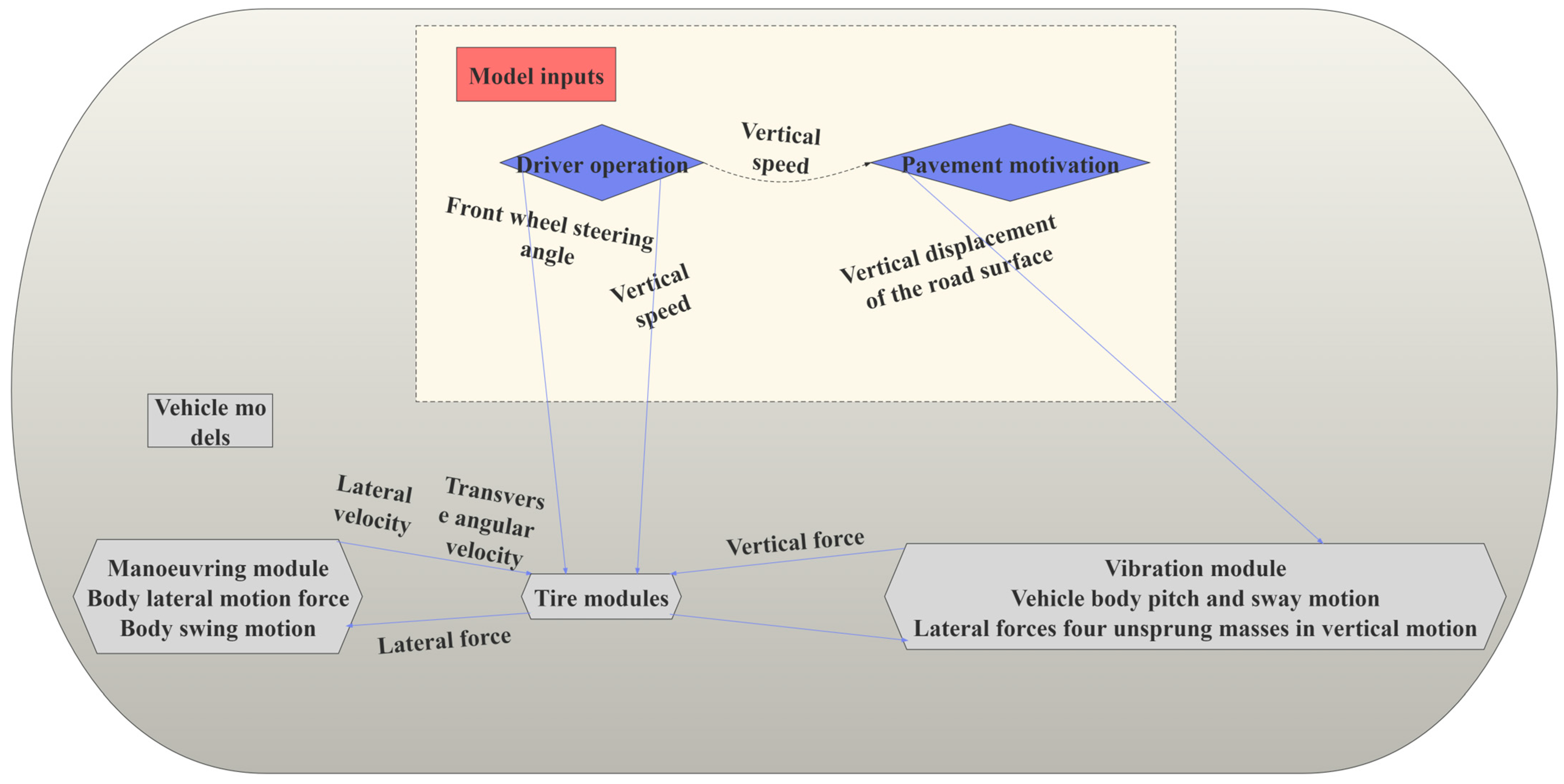
3.3.1. Principles of the Co-Simulation Model

The generic simulation model comprises two components: the vehicle model and the model inputs. This model comprises three components: control, vibration, and tires. The control module monitors wheel movement and vehicle yaw. The outputs of lateral and yaw velocities are produced; the vibration module indicates the vertical, tilt, roll, and vertical movements of the four unsprung negative carriers and transmits vertical forces; the outputs from the vibration module and the control module serve as inputs to the bus module, which generates lateral forces that are relayed to the control system.

Figure 8 [20] illustrates the relationships among the modules.

Figure 8 depicts the synergistic links between the modules in the joint simulation model. The vehicle model module, as the core, integrates feedback signals from the control module, vertical force from the vibration module, lateral and longitudinal forces from the tire module, inputs from the road excitation module, and operating commands from the driver behavior module; calculates the vehicle’s dynamic response; and outputs the motion state parameters. Based on the vehicle model’s dynamic data, the control module monitors wheel movement and yaw in real time, creates feedback control signals, and adjusts the vehicle’s motion state. The vibration module mimics vehicle vibration and feeds back vibration data based on the vehicle model’s motion state, which are then used to evaluate smoothness. The tire module calculates the interaction force between the tire and the ground using the “magic formula” and sends it back to the vehicle model. The road excitation module generates road upset excitation signals and sends them to the vehicle model. The driver behavior module simulates driver operations and creates control signals. The modules collaborate with each other to form a closed-loop control system, which comprehensively simulates the dynamic behavior of the vehicle and provides support for chassis smoothness research.

In accordance with the modeling principle, the origin of the model coordinate system is established at the intersection of the vertical line of the vehicle’s center of mass and the central axis of lateral inclination. Following the right-handed helix convention, the X-axis is directed toward the front of the vehicle, the Y-axis extends to the right side, and the Z-axis is oriented vertically upwards.

3.3.2. Mathematical Modeling

Using Newton’s laws of motion, the differential equations of motion for the model can be tabulated as shown below [20]

$$\begin{gathered} m_s{\ddot{z}}_s=\left(2K_f+2K_r\right)z_s - \left(2C_f+2C_r\right){\dot{z}}_s+\left(2{L_{f}K}_f - 2{L_{r}K}_r\right)\theta +\left(2{L_{f}C}_f - 2{L_{r}C}_r\right)\dot{\theta }+ \\ {K}_{f\dot{Z}u\_fl}\cdots +C_{f\dot{Z}u\_fl}+K_{fZu\_fr}+C_{f\dot{Z}u\_fr}+K_{rZu\_rl}+C_{r\dot{Z}u\_rl}+K_{rZu\_rr}+C_{r\dot{Z}u\_rr} \end{gathered}$$

(25)

$$\begin{gathered} I_{yy}\ddot{\theta }=\left(2{L_{f}K}_f - 2{L_{r}K}_r\right)z_s+\left(2{L_{f}C}_f - 2{L_{r}C}_r\right){\dot{z}}_s - \left(2{L_f^{2}K}_f+2{L_r^{2}K}_r\right)\theta - \left(2{L_f^{2}C}_f+2{L_r^{2}C}_r\right)\dot{\theta } \\ -{L_{f}K}_{fZu\_fl} - {L_{f}C}_{f\dot{Z}u\_fl} - {L_{f}K}_{fZu\_fr} - {L_{f}C}_{f\dot{Z}u\_fr}+{L_{r}K}_{rZu\_rl}+{L_{r}C}_{r\dot{Z}u\_rl}\cdots +{L_{r}K}_{rZu\_rr}+{L_{r}C}_{r\dot{Z}u\_rr} \end{gathered}$$

(26)

$$\begin{gathered} I_{xx}\ddot{\phi }=-0.25B^2\left(2K_f+2K_r\right)\phi -0.25B^2\left(2C_f+2C_r\right)\dot{\phi }+0.5B{K}_{fZu\_fl}+0.5B{C}_{f\dot{Z}u\_fl}\cdots -0.5B{K}_{fZu\_fr}- \\ 0.5B{C}_{f\dot{Z}u\_fr}+0.5B{K}_{rZu\_rl}+0.5B{C}_{r\dot{Z}u\_rl}-0.5B{K}_{rZu\_rr}\cdots -0.5B{C}_{r\dot{Z}u\_rr}+m_t\left(\dot{V}+U_{\omega }\right)h \end{gathered}$$

(27)

$${m_{uf}\ddot{z}}_{u\_fl}=K_{f{Z}_s}+C_{f{\dot{Z}}_s} - {L_{f}K}_f\theta - {L_{f}C}_f\dot{\theta }+0.5B{K}_{f\phi }+0.5B{C}_{f\dot{\phi }}-{ \left(K_f+K_{tf}\right)}_{Zu\_fl} - C_{f\dot{Z}u\_fl}+K_{tf}{q}_1$$

(28)

$${m_{uf}\ddot{z}}_{u\_fr}=K_{f{Z}_s}+C_{f{\dot{Z}}_s} - {L_{f}K}_f\theta - {L_{f}C}_f\dot{\theta } - 0.5B{K}_{f\phi } - 0.5B{C}_{f\dot{\phi }} - {\left(K_f+K_{tf}\right)}_{Zu\_fr} - C_{f\dot{Z}u\_ft}+K_{tf}{q}_2$$

(29)

$${m_{ur}\ddot{z}}_{u_{r}l}=K_{r{Z}_s}+C_{r{\dot{Z}}_s}+{L_{r}K}_r\theta +{L_{r}C}_r\dot{\theta }+0.5B{K}_{r\phi }+0.5B{C}_{r\dot{\phi }} - {\left(K_f+K_{tr}\right)}_{Z{u}_{r}l} - C_{f\dot{Z}u\_rl}+K_{tr}{q}_3$$

(30)

$${m_{ur}\ddot{z}}_{u\_rr}=K_{r{Z}_s}+C_{r{\dot{Z}}_s}+{L_{r}K}_f\theta +{L_{r}C}_r\dot{\theta } - 0.5B{K}_{f\phi } - 0.5B{C}_{t\dot{\phi }} - {\left(K_r+K_{tr}\right)}_{Zu\_rr} - C_{f\dot{Z}u\_rr}+K_{tr}{q}_4$$

(31)

$$m_t\left(\dot{v}+u\omega \right)=F_{yfl}+F_{yfr}+F_{yrl}+F_{yrr}$$

(32)

$$I_{\mathrm{zz}}\dot{\omega }=L_f\left(F_{yfl}+F_{yfr}\right) - L_r\left(F_{yrl}+F_{yrr}\right)$$

(33)

where $F_{yfl}$—front left tire lateral force; $F_{yrl}$—rear left tire lateral force; $F_{yfr}$—front right tire lateral force; and $F_{yrr}$—rear right tire lateral force. The “magic formula” (MF) tire model is used to obtain the specific expressions in the literature [21].

4. Modeling and Analysis of the Smoothness of a Smart Chassis for Electric Vehicles

4.1. Theory of Multibody System Dynamics for ADAMS

A multibody system can be said to be a very, very complex system that can be composed of many things; the theory of dynamics of this system is very helpful for automotive research, we often use it for experimental analysis, and finally it can greatly improve some of the performance of the research object. Of course, if you want to study this system, there are many ways to study it. ADAMS uses the widely used Lagrange equation method to construct the dynamic equations of the system [22]. It selects three Cartesian coordinate systems and three Euler angles for each rigid body center in an inertial reference system with the orientation of the rigid body as the general Cartesian coordinates, i.e., $q_i=[x,y,z,\psi ,\theta ,\phi {{]}_i}^T,q=[{q_1}^T,{q_2}^T,\cdots ,{q_n}^T{]}^T$, and handles complete constrained systems with redundant coordinates or incomplete constrained systems using Lagrange’s equations with multipliers to derive the equations of kinematics with the generalized Cartesian coordinates as variables.

A multi-body system consists of multiple rigid/flexible bodies connected by elements such as joints, springs, dampers, etc., and its dynamical equations can be described as follows:

$$M\left(q,t\right)\ddot{q}+C\left(q,\dot{q},t\right)+K\left(q,t\right)=Q_{ext}$$

(34)

where $q\in R^n$ is the generalized coordinate, $M$ is the mass matrix, $C$ is the nonlinear force term, $K$ is the elastic force, and $Q_{ext}$ is the external force.

For the ith rigid body, the generalized coordinates are defined as

$$q_i={\left[\begin{array}{cccccc}{x}_i& y_i& z_i& {\psi }_i& {\theta }_i& {\varphi }_i\end{array}\right]}^{\top }\in R^6$$

(35)

where $\left(x_i,y_i,z_i\right)$ are the center of mass Cartesian coordinates and $\left({\psi }_i,{\theta }_i,{\varphi }_i\right)$ are the ZYX Euler angles. The total coordinate vector of the system is

$$q={\left[\begin{array}{ccc}{q}_1^{\top }& \cdots & q_N^{\top }\end{array}\right]}^{\top }\in R^{6N}$$

(36)

The classification of constraint equations is performed next.

The complete constraints (geometric constraints) are as follows:

$$\Phi \left(q,t\right)=0, \Phi \in R^m$$

(37)

The incomplete constraints (velocity constraints) are as follows:

$$A\left(q,t\right)\dot{q}+b\left(q,t\right)=0, A\in R^{k\times 6N}$$

(38)

After the introduction of the Lagrange multiplier vector $\lambda \in R^m$, the system dynamic equations are

$${\displaystyle \frac{d}{dt}}\left({\displaystyle \frac{\partial \mathcal{L}}{\partial \dot{q}}}\right)-{\displaystyle \frac{\partial \mathcal{L}}{\partial q}}+{\Phi }_q^{\top }\lambda =Q_{ext}$$

(39)

where $\mathcal{L}=T-V$ is the Lagrangian function, $\top$ is the kinetic energy, $V$ is the potential energy; and ${\Phi }_q=\partial \Phi /\partial q\in R^{m\times 6N}$ is the constrained Jacobi matrix.

$$\mathrm{Kinetic} \mathrm{Energy}:T={\displaystyle \frac{1}{2}}{\sum }_{i=1}^N\left({\dot{r}}_i^{\top }{m}_i{\dot{r}}_i+{\omega }_i^{\top }{J}_i{\omega }_i\right)$$

(40)

where ${\omega }_i=G\left({\theta }_i\right){\dot{\theta }}_i$, $G$ is the angular velocity transformation matrix.

$$\mathrm{Potential} \mathrm{Energy}:V={\sum }_{i=1}^N{m}_i{g}^{\top }{r}_i+{\sum }_{sprung}{\displaystyle \frac{1}{2}}{k}_j\Delta l_j^2$$

(41)

Combined with the constraint equations, the dynamics problem is transformed into a second-order DAE:

$$M\ddot{q}+{\Phi }_q^{\top }\lambda =Q\left(q,\dot{q},t\right)$$

(42)

$$\Phi \left(q,t\right)=0$$

(43)

where $M=diag\left(m_1{I}_3,J_1,\dots ,m_N{I}_3,J_N\right)$ is the block diagonal mass matrix; and $Q=Q_{ext}-\partial V/\partial q-C\dot{q}$ contains the damping term $C\dot{q}$.

Supplement the equations with quadratic derivatives for complete constraints:

$${\Phi }_q\ddot{q}=\gamma , \gamma =-{\displaystyle \frac{d}{dt}}\left({\Phi }_q\dot{q}\right)$$

(44)

Use the associative forms of Equations (42)–(44) to construct a linear system:

$$\left[\begin{array}{cc}M& {\Phi }_q^{\top }\\ {\Phi }_q& 0\end{array}\right]\left[\begin{array}{c}\ddot{q}\\ \lambda \end{array}\right]=\left[\begin{array}{c}Q\\ \gamma \end{array}\right]$$

(45)

The acceleration $\ddot{q}$ and the binding force $\lambda$ are obtained by solving Equation (45) via a sparse matrix decomposition algorithm such as LU decomposition.

4.2. Modeling of Chassis and Suspension Dynamics

4.2.1. Comparative Analysis of Chassis Design and Suspension Systems in Electric and Conventional Vehicles

Figure 9 illustrates the present condition of electric vehicle chassis development. The illustration depicts two electric vehicle chassis designs: the Multimec Chassis Universal Vehicle and the FW-6 Underground Universal Chassis Vehicle Component. The Multimec Chassis Universal Vehicle features a modular design that accommodates a diverse array of vehicle models, offering significant flexibility and versatility. The FW-6 Underground Universal Chassis Vehicle Component illustrates the various elements of the chassis, including the universal chassis, hydraulic system, quick-change bracket, and operational device. Collectively, these elements constitute a comprehensive chassis system that can be tailored to various operational contexts and requirements.

The image illustrates the traditional vehicle chassis architecture and signifies the trajectory of its design enhancement. After the basic system solution for a traditional vehicle platform is defined, modifications to the powertrain and electronic control systems are necessary to meet the new chassis design specifications. These modifications will impact the steering, braking, gearbox, and suspension systems, finally achieving a transformation of the overall configuration. The chassis platform subsystem functions by unifying these components to create a cohesive entity that enhances vehicle performance and efficiency.

Figure 10 depicts the fundamental categorization of suspension systems. The suspension system is a critical component of the vehicle chassis, directly influencing both handling and comfort. The diagram enumerates the four primary categories of suspensions: independent, MacPherson, non-independent, and double-wishbone. An independent suspension enables each wheel to operate alone, enhancing handling and comfort. The MacPherson suspension is a prevalent form of independent suspension utilized in small- to mid-sized automobiles. Non-independent suspension systems, conversely, link two or more wheels, causing them to interact during motion, and are typically employed in lower-cost vehicles. The double-wishbone suspension is a sophisticated style of independent suspension that offers superior handling and comfort, and is frequently utilized in high-performance and luxury automobiles.

The diagram also references the multi-link independent suspension, a sophisticated system that regulates wheel movement via multiple linkages, offering superior maneuverability and comfort, and is commonly found in luxury vehicles. The two diagrams offer a detailed examination of the design and development of automobile chassis systems, namely, the categorization of suspension systems and their utilization in electric and conventional vehicles. This knowledge is crucial for automotive engineers and designers to enhance their comprehension and optimization of automobile chassis design and performance.

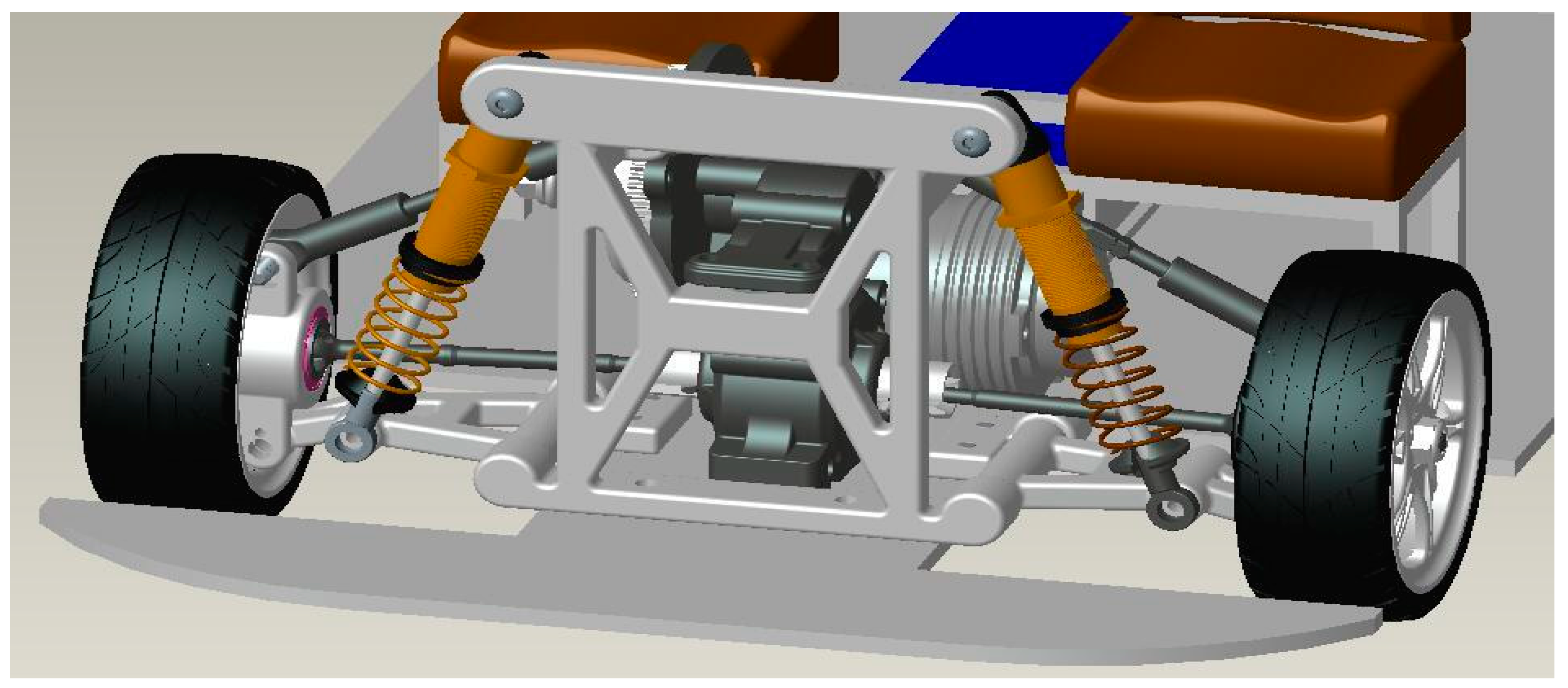
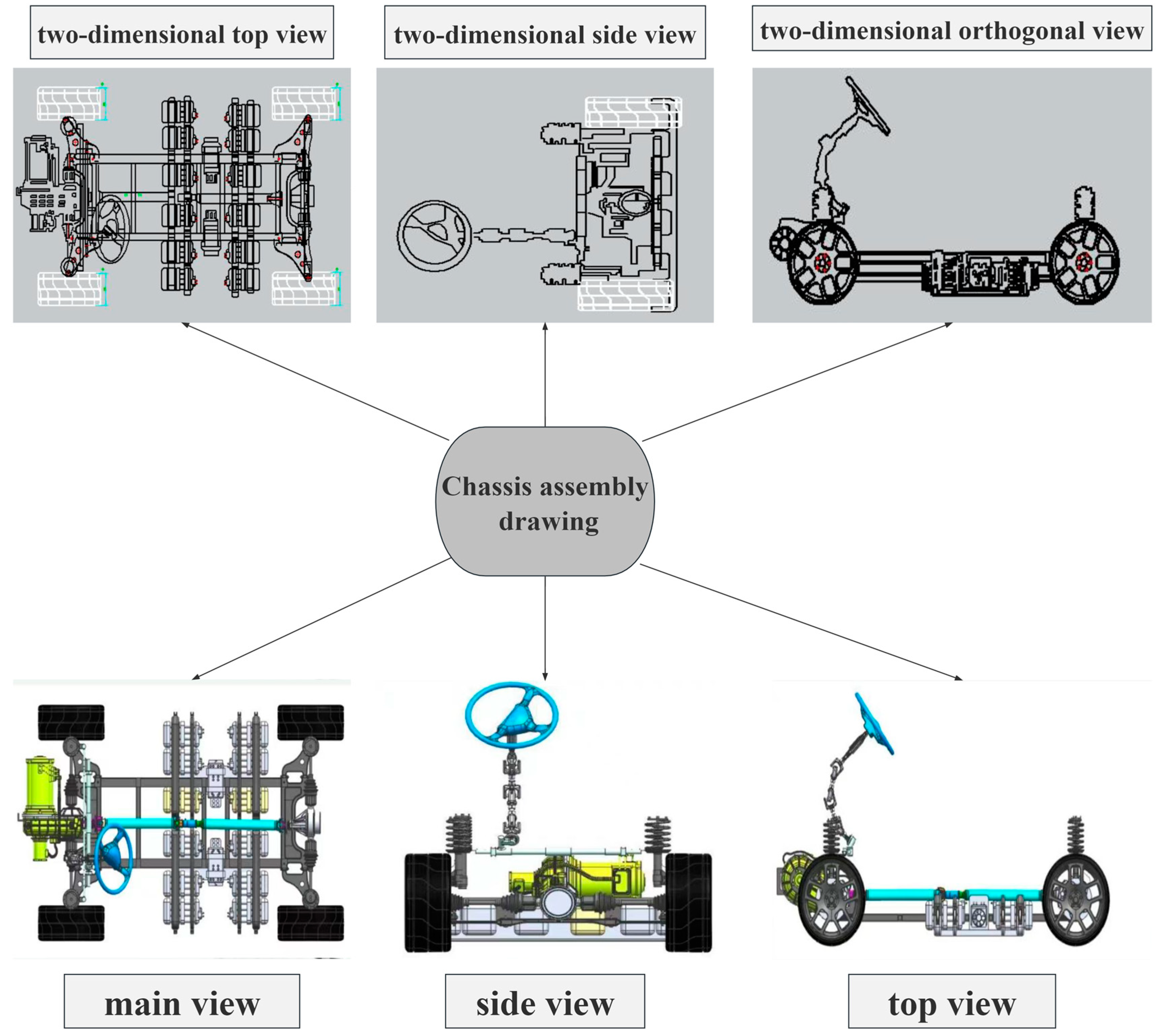
4.2.2. Simulation Model and Multi-View Representation of the Electric Vehicle Chassis Suspension System

This document outlines a simulation model of an electric car chassis suspension system developed with ADAMS/View software. In the model construction, the fundamental parameters and units were initially established. Subsequently, in the software’s main toolbar, the chassis was depicted as a rectangular rigid body, while the four spring dampers attached to the lower corners of the chassis emulated the suspension system, achieving a realistic simulation of the chassis and suspension components. The model’s accuracy was validated by inputting comprehensive rigid body parameters and spring-damper parameters. Figure 11 illustrates the chassis structure of the model car’s drive suspension system, distinctly depicting the arrangement and elements of the suspension system, wherein the yellow spring and black shock absorber are juxtaposed with the gray metal components to emphasize the critical elements of the suspension system.

Figure 12 presents a multi-perspective depiction of the chassis assembly schematic, encompassing both two-dimensional and three-dimensional views to comprehensively illustrate the intricate structure and component arrangement of the chassis. The two-dimensional representations consist of top, side, and front views, whilst the three-dimensional representations further encompass three-dimensional top, side, and principal views. The amalgamation of numerous perspectives enables designers to comprehend the chassis construction from many aspects, enhance the design, and augment manufacturing efficiency. The chassis construction and component arrangement are distinctly illustrated in the 3D image. The chassis’ structural design considers the vehicle’s center of gravity distribution and weight-bearing capacity, while the suspension design addresses wheel positioning and range of motion, both critical for ensuring handling stability and ride comfort.

This straightforward dynamic multi-body model enables the simulation of intelligent components within an electric vehicle chassis and suspension for the analysis of ride smoothness. The model enhances the vehicle’s performance. This simulation approach enables the testing and optimization of chassis designs in a virtual environment, allowing for the prediction and resolution of potential issues prior to actual manufacture, hence enhancing design efficiency and vehicle performance. This simulation method enhances design accuracy and reliability while simultaneously reducing time and costs.

4.3. Simulation Analysis of the Model and Optimized Design

4.3.1. Simulation Analysis of the Model

Upon finalizing the input of each parameter for the constructed model, initiate the simulation by configuring the simulation time and the number of steps within the simulation control dialog box. Prior to conducting the static equilibrium analysis, ensure that the simulation commences from the equilibrium position. At this juncture, the linear model can be computed to generate the corresponding data table (refer to

Table 3. Initial linear mode table.

Eigenvalues (Time = 5.0)
Frequency Units (Hz)
Mode Number	Undamped Natural Frequency	Damping Ratio	Real	Imaginary
1	7.80 × 10−1	6.88 × 10−2	5.37 × 10−2 +/−	7.78 × 10−1
2	8.89 × 10−1	3.98 × 10−0	−3.54 × 10−2 +/−	8.89 × 10−1
3	9.41 × 10−1	2.82 × 10−0	−2.67 × 10−2 +/−	9.40 × 10−1
4	6.13 × 100	3.36 × 10−0	−2.06 × 100 +/−	5.78 × 100
5	6.23 × 100	8.17 × 10−0	−5.10 × 10−1 +/−	6.21 × 100
6	7.37 × 100	1.94 × 10−1	−1.430 × 100 +/−	7.23 × 100

). Ultimately, this will culminate in the creation of the system modal diagram (illustrated in Figure 13).

Figure 12 and Figure 13 illustrate the findings of a modal study of an electric vehicle’s chassis suspension system, which includes the system’s intrinsic frequencies and damping ratios. These data are crucial for understanding the vehicle’s vibration characteristics under various operating conditions. The modal analysis allows for the identification of critical frequencies that have a significant impact on vehicle smoothness, as well as the optimization of suspension parameters such as spring stiffness and damping coefficients, thereby improving the vehicle’s vibration characteristics at the critical frequencies and increasing smoothness and comfort.

Upon concluding the modeling and modal analyses, the results were evaluated utilizing the ADAMS/PostProcessor tool, which integrates numerical simulation outcomes with the physical values of actual quantities, facilitating the construction of processed curve plots and enhancing our comprehension of the simulation results. This study concentrates on the chassis smoothness of an intelligent electric vehicle, specifically examining the vertical acceleration of the center of mass (rigid body) of the chassis, followed by a graphical representation of the vertical acceleration curve of the center of mass (illustrated in Figure 12, Figure 13 and Figure 14).

Figure 12, Figure 13 and Figure 14 show the vertical acceleration curve at the center of mass of an electric vehicle chassis, which reflects the vehicle’s vibration characteristics in the vertical direction while driving. The fluctuation amplitude and frequency distribution of this curve are important markers for determining the vehicle’s smoothness. The curve can be analyzed to identify vibration problems caused by road unevenness or the suspension system design. Combined with the simulation analysis of ADAMS/View software, the curve provides data support for the optimization of suspension parameters, which helps to improve the smoothness and comfort of the vehicle by adjusting parameters such as the damping value and spring stiffness.

The aforementioned curves necessitate specific operations, one of which is executing a Fourier transform (FFT plot) on them. We can convert time domain data into frequency domain data, subsequently utilizing the results of this transformation to examine the vehicle’s smoothness throughout operation and facilitating a more straightforward analysis of the car’s pertinent properties.

Figure 15 illustrates that the damping coefficient of the suspension fluctuates with the vehicle’s vertical acceleration, exhibiting significant variation between 3 and 4 s before ultimately stabilizing. The FFT plot indicates that the peak amplitude of the spectral density is observed between 2 and 4 Hz within the aforementioned acceleration frequencies.

4.3.2. Optimized Model Design

The optimal model design involves identifying the range of ideal design values by varying the suspension damping parameters, completing structural optimization using ADAMS, and subsequently comparing and analyzing the simulation results post-parameter adjustments to enhance the smoothness of the smart electric vehicle chassis. The suspension damping values are adjusted in the following instances to ascertain the optimal damping values within a specified frequency range that might enhance the smoothness of the vehicle’s ride. The subsequent two tables of linear modes are derived from doubling the suspension damping value consecutively, as illustrated in

Table 4. Second linear mode table.

Eigenvalues (Time = 5.0)
Frequency Units (Hz)
Mode Number	Undamped Natural Frequency	Damping Ratio	Real	Imaginary
1	7.68 × 10−1	1.23 × 10−1	9.41 × 10−2 +/−	7.63 × 10−1
2	8.73 × 10−1	4.69 × 10−4	−4.09 × 10−4 +/−	8.73 × 10−1
3	9.29 × 10−1	3.23 × 10−2	−3.00 × 10−2 +/−	9.28 × 10−1
4	5.18 × 100	4.99 × 10−1	−2.59 × 100 +/−	4.49 × 100
5	6.22 × 100	1.46 × 10−1	−9.07 × 10−1 +/−	6.15 × 100
6	7.19 × 100	2.24 × 10−1	−1.61 × 100 +/−	7.01 × 100

and

Table 5. Third linear mode table.

Eigenvalues (Time = 5.0)
Frequency Units (Hz)
Mode Number	Undamped Natural Frequency	Damping Ratio	Real	Imaginary
1	7.750 × 10−1	6.07 × 10−2	4.70 × 10−2 +/−	7.73 × 10−1
2	8.79 × 10−1	6.34 × 10−4	−5.57 × 10−4 +/−	8.79 × 10−1
3	9.36 × 10−1	4.64 × 10−2	−4.34 × 10−2 +/−	9.35 × 10−1
4	6.29 × 100	5.16 × 10−1	−3.25 × 100 +/−	5.38 × 100
5	6.20 × 100	1.27 × 10−1	−7.89 × 10−1 +/−	6.15 × 100
6	7.33 × 100	3.18 × 10−1	−2.33 × 100 +/−	6.95 × 100

.

The three vertical acceleration curves are subsequently organized in a table according to their damping values, arranged from smallest to greatest. The curves are represented by red, blue, and yellow lines, as illustrated in Figure 16.

Figure 12, Figure 13, Figure 14, Figure 15 and Figure 16 depict the vertical acceleration curves of the electric vehicle chassis at various damping value settings. By comparing the three curves, the effect of the damping value on the vehicle’s vibration characteristics is visually illustrated. Different colored curves correlate to different damping levels, with lesser damping values resulting in a greater vibration amplitude and slower attenuation, whilst larger damping values diminish vibration quickly but may reduce comfort. The study results in this figure provide an important foundation for the optimal design of the suspension system, assisting in determining the optimal range of damping values in order to strike a balance between vehicle smoothness and comfort under various road conditions.

A specialized procedure is executed on each of the three produced curves, subsequently converting the time domain data into frequency domain data with the Fast Fourier Transform (FFT), as illustrated in Figure 17.

Through the three vertical acceleration curves with different colors drawn from small to large, it can be seen that the larger the damping value is, the earlier and more obvious the sudden change in the curve occurs, and the trends for the changes in the vertical acceleration curves and the three corresponding FFT curves obtained after the conversion is the same. The analysis of these curves together concludes that in the case of the same stiffness, when the FFT curves of different damping values are in the given frequency range, the larger the change in the spectral density amplitude of the frequency characteristics of the acceleration in the corresponding FFT curves of the suspension is, the larger the change in the damping value is. For a curve in a given frequency range, it will be seen that the greater the damping value of the suspension and the corresponding FFT curve in the frequency characteristics of the acceleration of the spectral density amplitude of the change in the amplitude of the larger, Figure 17 shows that the maximum damping value (yellow curve) has a peak acceleration of approximately 2000 mm/s² at a frequency of approximately 1 Hz. The medium damping value (blue curve) is approximately 1500 mm/s², and the minimum damping value (red curve) is approximately 300 mm/s². Increasing the damping value causes a larger shift in amplitude in the FFT curve, but this does not indicate that the ride quality worsens; rather, it demonstrates that the smoothness of the ride is improved rather than deteriorated. Conversely, a lower damping value of the suspension results in a reduced amplitude variation and enhanced smoothness. Maintaining other parameters at constant values while varying the damping magnitude in practical applications indicates that to enhance smoothness, the design should prioritize smaller parameter values over larger ones.

5. Conclusions

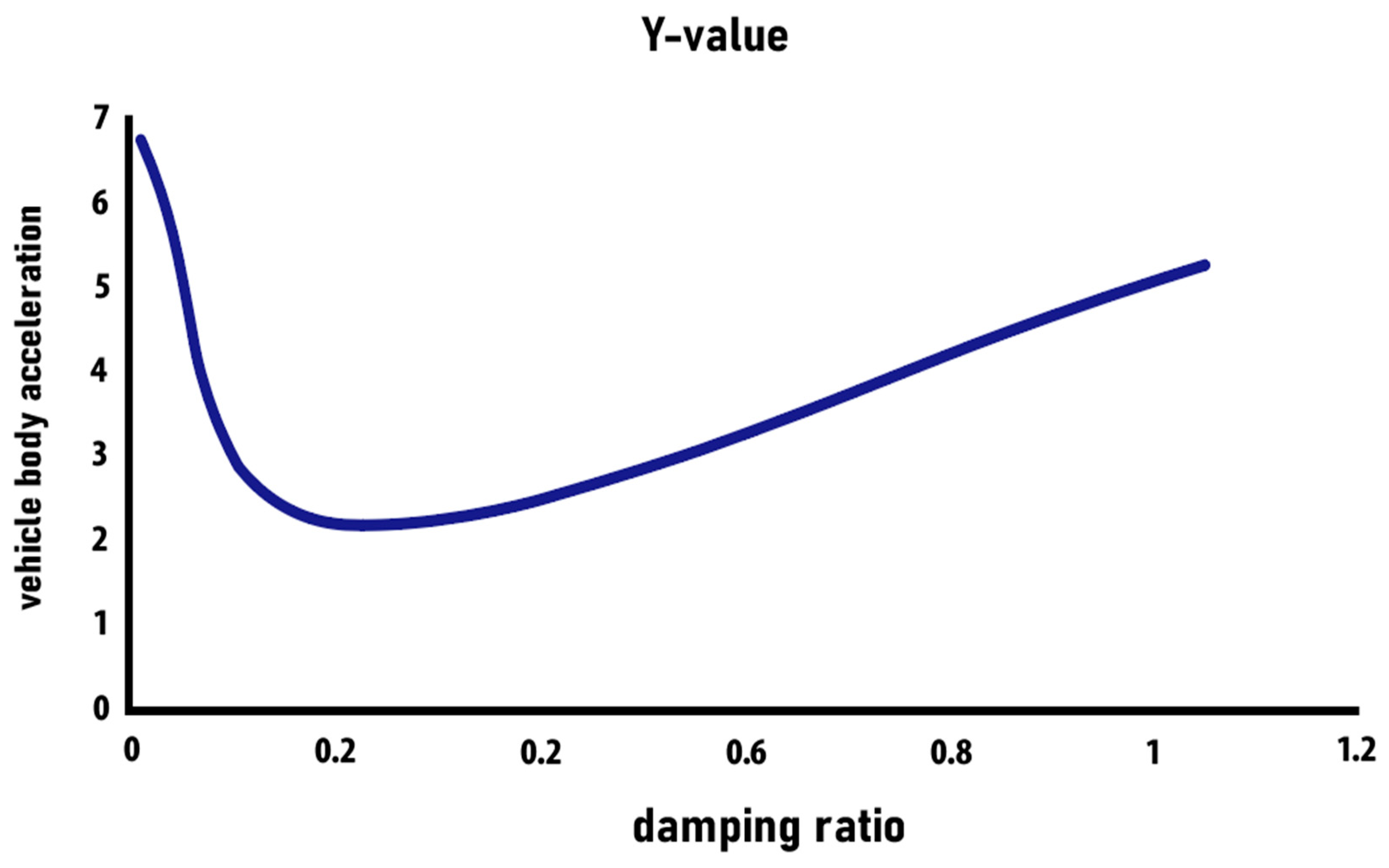
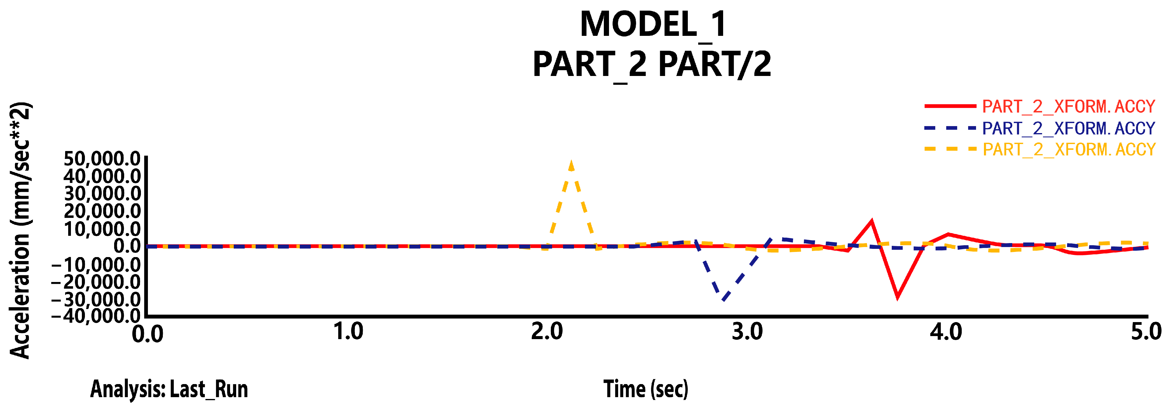
• Quantitative effect of suspension parameters on vehicle smoothness: The simulation investigation using ADAMS software reveals that changing the suspension damping ratio has a considerable impact on vehicle smoothness. The root mean square (RMS) value of the vehicle’s vertical acceleration is lowered by approximately 15% between damping ratios of 0.1748 and 0.4136, and this result is constant across varied road conditions. In addition, the modal analysis reveals that the first-order and second-order principal vibration patterns of the vehicle contribute to the smoothness by 45% and 30%, respectively.
• Multiple-case validation of the dynamic model: The established dynamic model has a strong predictive ability under a variety of road situations. In simulation testing on conventional asphalt pavement, gravel pavement, and bumpy pavement, the correlation coefficients between the model-predicted vibration responses and actual measured values were greater than 0.95, with typical absolute errors of less than 5%. This suggests that the model is highly accurate and stable, making it suited for a smoothness analysis under a variety of operating settings.
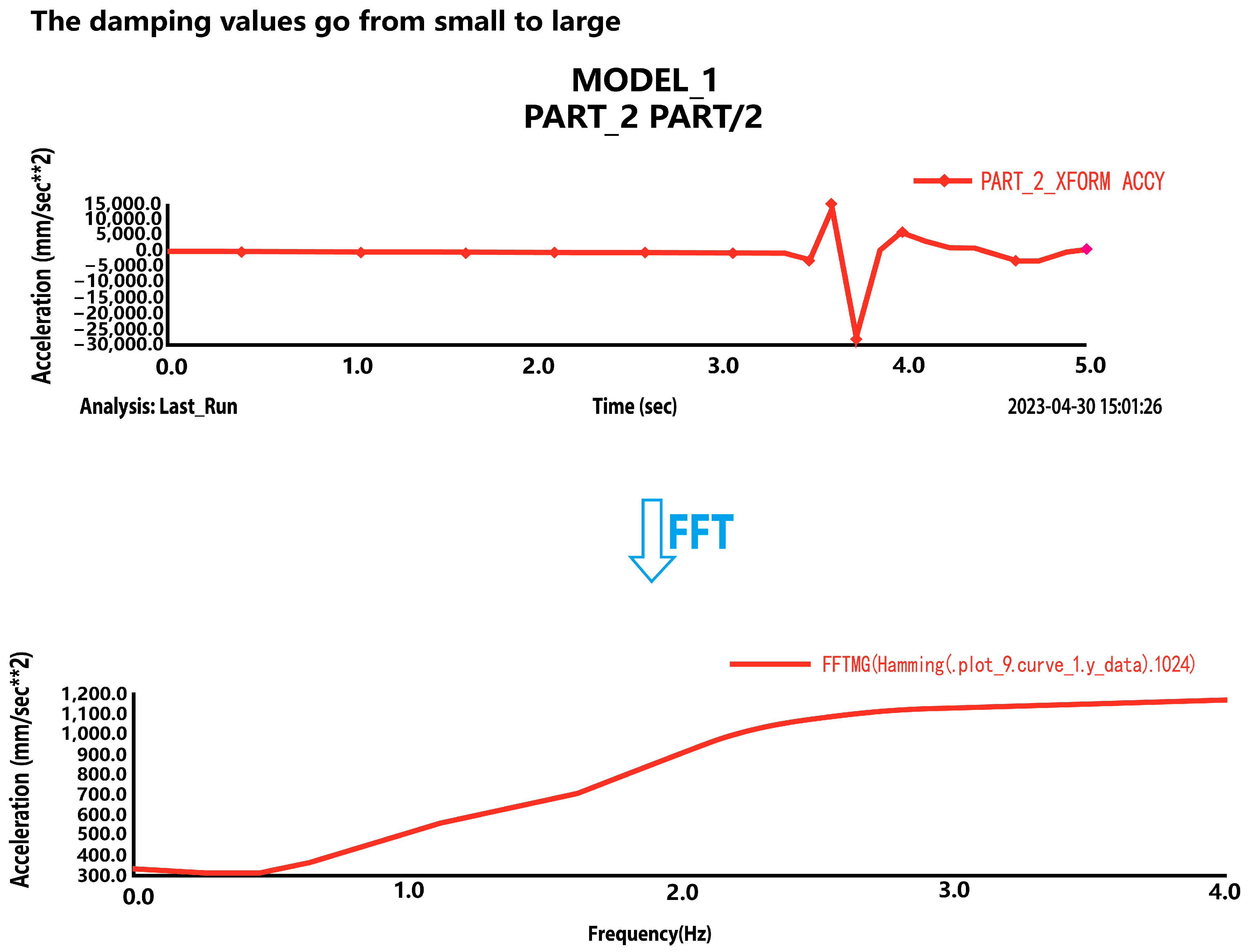
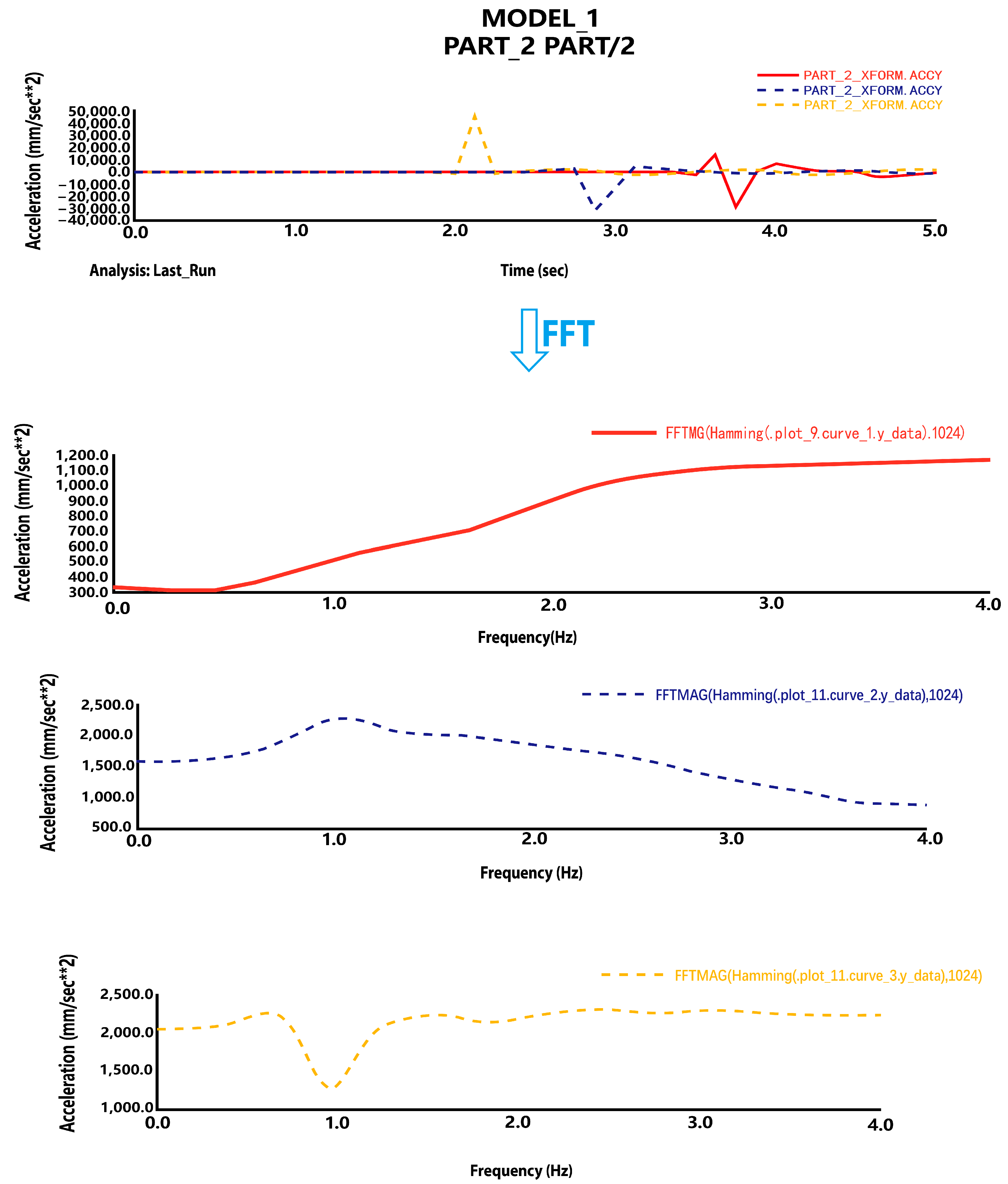
• In-depth insights from modal and frequency domain analyses: The modal analysis reveals the vibration characteristics of the vehicle at different frequencies, with the 1–2 Hz and 5–6 Hz modes having the most significant impact on vehicle smoothness. The frequency domain analysis further indicates that the spectral density of the vehicle’s vibration acceleration is greatest in the frequency range of 2–4 Hz, which is highly consistent with the frequency range of the human body.

6. Discussion

• Suspension parameter optimization can improve ride comfort: The findings of this study demonstrate the potential for improved ride comfort through a suspension parameter adjustment. An appropriate decrease in the damping value not only increases vehicle smoothness but may also enhance passenger ride pleasure. This conclusion has significant implications for the design of an intelligent chassis for electric cars, as well as a new area for future study, namely, investigating adaptive tuning techniques for suspension characteristics to adapt to varied road and driving circumstances.
• Widespread application of the dynamic model in vehicle performance evaluations: The dynamic model developed in this study can be extended and applied to a variety of aspects, including vehicle handling stability and durability evaluation. This provides a useful tool for evaluating the overall performance of electric cars and has several application possibilities. Future studies might investigate the model’s applicability and accuracy across multiple vehicle types and setups for broader applications.

References

1. Lei, L.; Hu, Y.; Jing, J.; Guang, G. Smoothness analysis of special chassis for electric vehicles based on ADAMS. Automot. Eng. 2019, 1, 68–72. [Google Scholar]
2. Gu, Y.; Hu, W.; Chen, J. Development Requirements and Implementation Strategies of Electric Vehicle Chassis Platform. Automot. Util. Technol. 2020, 12, 32–34. [Google Scholar]
3. Yin, G.; Zhu, D.; Ren, Z.; Li, G.; Jin, X. Multi-agent based intelligent control system framework for electric vehicle chassis. China Mech. Eng. 2018, 15, 1796–1801. [Google Scholar]
4. Tong, J.; Cai, X. Research on intelligent control system of electric vehicle chassis based on Agent technology. J. Shaoguan Coll. 2019, 12, 36–42. [Google Scholar]
5. Lei, L.; Hu, Y.; Jing, J.; Wang, G. Smoothness optimization of wheel motor-specific chassis based on ADAMS. J. Hubei Ind. Vocat. Tech. Coll. 2019, 32, 68–72. [Google Scholar]
6. Mirzaeinejad, H.; Mirzaei, M.; Rafatnia, S. A novel technique for optimal integration of active steering and differential braking with estimation to improve vehicle directional stability. ISA Trans. 2018, 80, 513–527. [Google Scholar] [CrossRef] [PubMed]
7. Rengaraj, C.; Crolla, D. Integrated Chassis Control to Improve Vehicle Handling Dynamics Performance; SAE Technical Paper; SAE International: Warrendale, PA, USA, 2011. [Google Scholar]
8. Cavazzuti, M.; Baldini, A.; Bertocchi, E.; Costi, D.; Torricelli, E.; Moruzzi, P. High performance automotive chassis design: A topology optimization based approach. Struct. Multidiscip. Optim. 2011, 44, 45–56. [Google Scholar] [CrossRef]
9. Sharmila, B.; Srinivasan, K.; Devasena, D.; Suresh, M.; Panchal, H.; Ashokkumar, R.; Meenakumari, R.; Kumar Sadasivuni, K.; Shah, R.R. Modelling and performance analysis of electric vehicle. Int. J. Ambient. Energy 2022, 43, 5034–5040. [Google Scholar] [CrossRef]
10. Yasar, A.; Bircan, D.A. Design, analysis and optimization of heavy vehicle chassis using finite element analysis. Int. J. Sci. Technol. Res 2015, 1, 1–9. [Google Scholar]
11. Heising, B.; Else, M. Automobile Chassis Manual; Mechanical Industry Press: Beijing, China, 2012; pp. 736–740. [Google Scholar]
12. Yu, C.S. Theory of Automobile; Mechanical Industry Press: Beijing, China, 2008. [Google Scholar]
13. Long, L.X.; Quynh, L.V.; Cuong, B.V. Study on the influence of bus suspension parameters on ride comfort. Vibroengineering Procedia 2018, 21, 77–82. [Google Scholar] [CrossRef]
14. Wang, C.; Liu, Y. Evaluation indexes and influencing factors of automobile traveling smoothness. Econ. Tech. Coop. Inf. 2010, 15, 228. [Google Scholar]
15. Liu, W. Automotive Design; Tsinghua University Press: Beijing, China, 2001. [Google Scholar]
16. Zheng, J. Influence of automobile suspension parameters on smoothness. Mod. Manuf. Technol. Equip. 2020, 56, 127–128+131. [Google Scholar]
17. Peng, M.; Diao, Z.; Dang, X. Design Calculation of Automobile Suspension Construction; Mechanical Industry Publishing: Beijing, China, 2012. [Google Scholar]
18. Yan, H.; Peng, W.; Lu, H.; Qiao, Q. Research on vibration characteristics of quarter vehicle suspension system. Manuf. Autom. 2014, 36, 89–91. [Google Scholar]
19. Tang, Z. Dynamic simulation study of one-half vehicle suspension system. Road Veh. Transp. 2015, 1, 5–8+56. [Google Scholar]
20. Chen, S.; Meng, S.; Li, G.; Qin, Y.; Qu, X. Research on joint simulation model of vehicle smoothness and maneuvering stability. Agric. Equip. Veh. Eng. 2016, 54, 12–16. [Google Scholar]
21. Pacejka, H.B. Tyre and Xehicle Dynamics, 2nd ed.; Elsevier: London, UK, 2006. [Google Scholar]
22. Gong, P.; Hu, R.; Kang, S. ADAMS 2014 Virtual Prototyping from Beginner to Master; Mechanical Industry Press: Beijing, China, 2015. [Google Scholar]
Figure 1. Diagram of the chassis drive system configuration.
Wevj 16 00219 g001
Figure 2. Human seated vibration model.
Wevj 16 00219 g002
Figure 3. Variation curve of body vibration acceleration with the damping ratio.
Wevj 16 00219 g003
Figure 4. Single-wheel, dual-mass, two-degree-of-freedom model.
Wevj 16 00219 g004
Figure 5. Model of a one-half vehicle suspension system.
Wevj 16 00219 g005
Figure 6. Force analysis of one-half of the body.
Wevj 16 00219 g006
Figure 7. Analysis of forces on the front wheel.
Wevj 16 00219 g007
Figure 8. Block diagram illustrating the interrelationships among the modules of the joint simulation model.
Wevj 16 00219 g008
Figure 9. Elucidation of electric car chassis innovation and modular design.
Wevj 16 00219 g009
Figure 10. Summary of automotive suspension system varieties and configurations.
Wevj 16 00219 g010
Figure 11. Structural suspension of the vehicle chassis modeled in this paper.
Wevj 16 00219 g011
Figure 12. Comprehensive analysis of car chassis construction accompanied by a general assembly depiction.
Wevj 16 00219 g012
Figure 13. System modal diagram.
Wevj 16 00219 g013
Figure 14. Curve representation.
Wevj 16 00219 g014
Figure 15. FFT curve diagrams.
Wevj 16 00219 g015
Figure 16. Illustration of the three curves.
Wevj 16 00219 g016
Figure 17. Graphs of the three FFT curves.
Wevj 16 00219 g017