Abstract
Detecting the spatial-temporal dynamics mechanisms and driving forces of ecological land change will offer a scientific basis for the sustainable utilization and ecological protection of regions undergoing rapid urbanization. This study examined the variations in ecological land from 2000 to 2015 in Yingkou by spatial statistical analysis with four land use/cover maps (2000, 2005, 2010, and 2015) interpreted by Landsat Thematic Mapper images and Google Earth maps. This study also measured the varying spatiotemporal drivers of typical ecological land use/cover types by survival analysis. The results indicated that ecological land was the main land use/cover type, and that the area decreased over time with a large transformation into agriculture and urban lands with significant temporal dynamics. The driving mechanisms became more complicated over time, and different time-dependent covariates significantly impacted the ecological land, forest land, and wetland losses. However, the distance from the city and different ways were the most important influencing spatiotemporal variables of the loss of ecological land, forest land, and wetlands over time. This study demonstrated the combined influence of a series of factors on ecological land loss. The spatial determinants and their impacts varied over time, especially the accessibility factors.
1. Introduction
Land use has undergone fundamental changes and it has substantially influenced biogeochemical and hydrological cycles, regional environment, biodiversity, and ecosystem services [1,2,3,4]. The world, especially the developing country of China, has experienced dramatic land use/cover changes and growing conflicts between economic development and conservation in the recent decades [5,6,7]. Studies on land use/cover change have focused on changes to types of land use and land production, rather than the variations in the land’s ecological functions [5,8]. Reasonable methodologies of land use classification and monitoring programs have emphasized the notion that ecological functions should be adopted to manage natural resources, monitor the impact of urbanization and human activities on the ecological environment, and coordinate the relationship between production, livelihood, and ecological functions [9,10]. Some studies have categorized land use/cover types into agricultural, urban, and ecological lands [5,6]. In this frame, ecological lands, including forest land, wetlands, grassland, orchards, and other natural land use/cover types can maintain the ecological process, balance the regional ecosystem, meet reasonable human needs, and improve the quality of human lives [10,11,12]. However, the causes, patterns, processes, and consequences of ecological land change still require further study. Identifying the driving forces of ecological land change is still essential to understanding the characteristics of the changes in order to mitigate the negative effects, promote the desired outcome, and protect natural resources in land-use planning.
The driving mechanisms of change to different ecological land types have been explored in some areas, such as forest land [13,14,15], wetlands [16,17], and ecological land [8,11,18]. However, the driving mechanisms and factors of change differ for dissimilar ecological land types from a regional perspective, due to land use type features, the natural environment, and human activities [8]. Thus, changes in different ecological land types have been rarely discussed. Ecological land, which is an important natural resource, is strongly influenced by the combination of the natural/spatial underlying factors, socio-economic factors, cultural factors, and land-use planning, rather than a single key variable [8]. Physical factors, such as elevation and slope have been considered as generally restrictive factors to ecological land, and ecological land with flat slopes and lower elevation, which are more likely to be exploited into becoming agriculture land and urban land [8,11,19,20]. Socio-economic factors, such as population and gross domestic product (GDP) have frequently affected ecological land change in two ways [5,8]. On one hand, with rapid urbanization and economic development, populations move from the countryside to urban areas, and the conflict between regional construction land and ecological protection increases. On the other hand, people begin to enjoy holidays in rural areas with economic developments, which also affects regional ecological land patterns. Proximity factors (i.e., distance to city, distance to towns, and distance to residential lands) impact on the ecological land through locational effects on a small scale in that ecological land near areas with intensive human activities are most greatly affected by the living and production benefits of human beings [8,11,18]. Frequently, accessibility factors (i.e., distance to national ways, province ways, and county ways) guide the expansion of urban and agriculture land and promote the land-use demand of different populations through influence on land price, and then they influence the spatial distribution of regional ecological land [8,21]. Land-use policy and urban planning (i.e., conservation area and land use policy) also influence ecological land change [3,13,22,23]. Climatic and hydrological conditions (i.e., annual rainfall, evaporation, quantity of inflow water) [16], soil organic matter [8], and other factors have also been linked to ecological changes. These factors might be the main determinants of the ecological land use/cover changes at the regional scale [24], especially in the region of China [8,11,18]. Therefore, these driving factors for measuring the varying spatiotemporal forces of ecological land in the study area are the focus of this study.
Many mathematical approaches, such as literature reviews [25,26], reasoning [27,28], regressions [29,30], and spatial statistical models [31] have been developed to examine the relationship between land use/cover and the influencing factors. Mostly regression models are used, such as the logistic model [11], binary logistic regression [18], stepwise logistic regression [20], partial least square regression [5], and the spatial analysis model [8,32]. Driving forces are identified at different times and regions by using these models. These approaches identify the main explanatory variables over a specified period without considering the long-term temporal changes in different periods. Whilst the driving forces of ecological land identified in different studies seem to be different, it is natural to develop the question: do the driving forces of ecological land change vary spatially and temporally? Few studies have shown that the driving force of ecological land varies based on the analyses of data in various models used over different time periods [11]. However, the measurement of varying spatiotemporal forces of ecological land use/cover change by one model is rarely studied. Therefore, efficient methods must be introduced to determine and to evaluate the dynamic driving forces of ecological land change quantitatively.
Survival analyses have comprehensively considered the occurrence and timing of a research event, which have been beneficial for longitudinal research that handles censoring and time-varying explanatory variables, and that are superior to conventional statistical methods [33,34,35]. The Cox hazard regression (a semi-parametric model for survival analysis) can easily incorporate time-dependent covariates that may change over time [35,36]. Survival analysis is extremely useful for studying different kinds of events in natural and social sciences, such as the recovery of patients, animal death [37], and deforestation [38,39]. An efficient approach is to analyze the varying spatiotemporal forces of land use/cover change [33,34,40] in order to identify the varying drivers and their effects.
To mitigate the negative effects of ecological land change, the varying driving forces of ecological land loss and their spatiotemporal features in Yingkou City were identified. Specifically, this study aimed to (1) investigate the ecological land change in Yingkou from 2000 to 2010, (2) quantify the varying spatiotemporal drivers of ecological land loss by survival analysis using the Cox hazard model with time-dependent variables, and (3) offer a scientific basis for natural resource protection and ecosystem strengthening.
2. Materials and Methods
2.1. Study Area and Data Processing
The Yingkou region (39°55′ N–40°56′ N and 121°56′ E–123°02′ E) is in the Northwestern part of Liaodong Peninsula, China (Figure 1). The region covers 527,500 ha, and mountainous areas account for approximately 50% of the area. Benefiting from these topographic and geography features, the area has abundant forest and wetland resources, making up about 46% and 6% of the total area, respectively [41]. Over the past 15 years, the region has undergone remarkably rapid economic growth and urbanization, and a considerable decrease in forest land and wetlands [41]. Therefore, the natural resources should be analyzed and monitored in Yingkou, to protect natural environment and ecosystem processes.
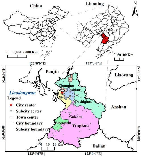
Figure 1.
Location of the study area in China.
The land use/cover data with a pixel size of 30 × 30 m in 2000, 2005, 2010, and 2015 were sources from the study of Liu et al. (2016) and Zhang et al. (2017), interpreted based on Landsat Thematic Mapper images and Google Earth maps using the ENVI 5.1 software. These land use/cover maps represent the same data sources, processing methods, and classification systems, and they are the most appropriate data to identify changes in land use/cover. Overall accuracies were approximately 90% and the Kappa coefficient was 0.8 [41,42]. The land use/cover classification system included cropland, forest land, urban land, wetlands, and other land. In this classification, other land comprised grassland, bare land, and so on, which are less disturbed by human activities. In this study, the land use/cover classes were divided into three sub-types (i.e., ecological, agricultural, and urban lands) according to their land functions, and natural or human disturbance characteristics using the ESRI ArcGIS 10.2 software. Ecological lands, including forest land, wetlands, and other natural land provide ecological goods and services, and have natural characteristics [5]. The spatial distribution of land use/cover types is shown in Figure 2.
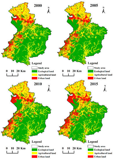
Figure 2.
Distributions of land use/cover types of Yingkou, China in 2000, 2005, 2010, and 2015.
2.2. Ecological Land Change Assessment
Ecological land use/cover changes were analyzed using four land-use maps with the same land use/cover classification system for the reference years 2000, 2005, 2010, and 2015, by spatial statistical analysis. The spatial statistic (i.e., cross-tabulation analysis) was used to construct the transfer matrix of land use/cover by overlaying and intersecting land use/cover maps [43,44] to reflect the area change between the ecological land use/cover and non-ecological land during the 2000–2005, 2005–2010, and 2010–2015 periods in Yingkou.
Ecosystem service values (ESV) were also calculated to reflect the ecosystem functions change of ecological lands, which can be expressed as follows [45]:
where ESV indicates the total value of the ecosystem services in the ecological land; donates the area of the ecological land i (i.e., forest land, wetlands, and other natural land); VC signifies the valuation coefficients of ecosystem services j in ecological land i. The value coefficients for ecosystem services of different ecological land use/cover were calculated by the evaluation method for ecosystem service values based on a per unit area [45].
2.3. Driving Forces
Landscape change is affected by distinct combinations of cultural, political, and natural drivers [46]. Many studies have recognized the analytical framework of the influencing factors of ecological land change, the variables of which were considered in the survival analysis in the current study with the available data (Table 1 and Figure 3). (1) Elevation and slope are generally restrictive factors of ecological land, which may change in the area with flat slope and low elevation [8]. (2) Two socio-economic factors, population and GDP [5,8], affect land change because the conflict between regional construction land and ecological protection increases with rapid urbanization and economic development. (3) Three proximity factors; namely, distance to city, distance to towns, and distance to residential lands [8,11,18], affect ecological lands through locational effects on a small scale; that is, ecological lands near intensive human activity areas are expected to be most greatly affected by the living and production benefits of human beings. (4) Three accessibility factors, namely, the distance to national, province, and county ways [21] impact land use/cover in promoting the land use/cover demand of different populations by influencing the land price. All variables were normalized into [0, 1] with a z-score standardization method and used as the data for determining the drivers of ecological land change.

Table 1.
Selected preliminary variables for studying the driving forces of ecological land change.
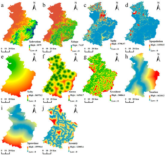
Figure 3.
Driving factors of spatial variables for the implementation of models (2000).
2.4. Survival Analysis
A survival analysis can be used to investigate the occurrence and timing of events such as land use/cover change for a specific period [47]. For ecological land loss, the conversion of land units from ecological land to other types is equivalent to an individual death event, which indicates that the survival time of an ecological land cell is the time duration until its state conversion [40].
In the survival analysis, the unchanged probability of ecological land can be calculated using the following formula [34]:
where T represents the time for ecological land unchanged, represents the cumulative unchanged rate of ecological land, which implies that the ecological land remains unchanged after the observation time t, represents the probability of ecological land that is unchanged. The derivative of is equivalent to the hazard function:
where represents the risk rate of ecological land loss between t and (), given that the ecological land is unchanged over time t.
In measuring the time-varying characteristics of the spatial driving factors, the Cox model with time-independent covariates was used to obtain [48]. The proportional hazard model with time-dependent covariates, as an extension of the Cox model, is usually written as [35]:
The formula can also be expressed as follows:
where represents the probability of ecological land loss over time t, denotes the baseline hazard function, which is related to t but is not the variable, represents the time-dependent variables, and it is sometimes expressed as [40], and are the regression coefficients for the variables. are the regression coefficients for the time-dependent variables.
The time variable t was discretized into several periods (2000–2005, 2005–2010, and 2010–2015) according to land use/cover, due to the difficulty in obtaining the time of land use/cover change. The changing state of ecological land loss was coded as a chain: 0000, 1000, 1100, 1110, and 1111. The model requires the observations to be censored, such as left, interval, and right censored data [34]. The forms of censored observations depend on whether and when the ecological land loss occurs (Figure 4). A combination of systematic and random sampling schemes was used to minimize autocorrelation, and to maintain the representativeness of the samples [33,49].
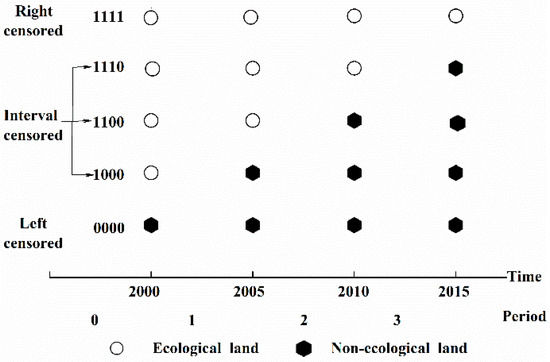
Figure 4.
Illustration of the forms of observations.
The Cox regression model was implemented on the basis of statistical software SAS9.4. Three formulas (i.e., BRESLOW, EFRON, and EXACT methods) can be alternated to handle the tied data in which two events occur simultaneously. Schoenfeld residuals were used to detect possible departures from the proportional hazard assumption [50]. If the assumption test is significant for whether the Schoenfeld residuals are correlated with time or some function of time, then the Schoenfeld residuals should be independent of time. Therefore, the correlation analysis between the Schonefeld residuals of spatial variable and time variable t was used to identify the time-dependent variable xik (t) for different types of ecological land. Three alternative variables, namely, a likelihood-ratio test, a score test and a Wald test, were used to display the null hypothesis that all coefficients were 0 [35]. The −2 log likelihood, Alaile’s information criterion (AIC), and Schwartz’s Bayesian criterion statistics were used to measure the fit of the models. A comparison of the fitted statistics can be used to choose an improved performance model with a low value in order to explore the driving forces of ecological land loss effectively.
3. Results and Discussion
3.1. Ecological Land Change
The amount of land use/cover changed between ecological land and non-ecological land during 2000–2005, 2005–2010, and 2010–2015 are shown in Table 2 and Table 3. Ecological land was the main land use/cover type and it accounted for over 50% of the total area in four years. Forest land was the main component of ecological land, followed by wetlands. It accounted for over 80% of the ecological land. The proportional area of ecological land decreased from 55.02% to 51.76%, with an area of 17,110.6 ha. Each type of ecological land showed a decreasing trend except for water in 2005 and other lands in 2010.
Table 2.
Ecological land use/cover types in Yingkou from 2000 to 2015 (ha, %).
Table 3.
Transfer matrix between ecological land and non-ecological in Yingkou (ha).
Over the last 15 years, Yingkou has experienced considerable ecological land loss, with 1528.64 ha in 2000 to 11,420 ha in 2015, and smaller gains, with 919.73 ha in 2000 to 2292.48 ha in 2015 (Table 3). Most of the ecological lands in the Western area were transformed into urban lands from 2000 to 2010, whereas most of the scattered ecological lands were transformed into agricultural lands in 2010–2015 (Table 3 and Figure 5). The lost wetlands, which were concentrated in the Northwest coastal regions, were transformed into new urban lands through the reclamation of sea and water regions from 2005 to 2010. The lost forest lands, which were located in the Northern central area, were transformed into urban lands in 2000–2005, and to agricultural land in 2005–2015.
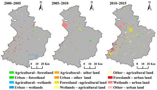
Figure 5.
Sampling points for ecological loss between 2000 and 2015 in Yingkou.
The ecosystem services in ecological land in Yingkou were 37,645 million in 2000 and they reduced to 22,318 million in 2005, increased to 39,303 million in 2010, and reduced to 27,846 million in 2015 (Table 4). The trend was mainly dominated by forest land, due to its occupation of a higher proportion of area and the coefficient ecosystem services. This trend indicated that the ecosystem service values of Yingkou had a fluctuating trend, which was not only impacted by the decreased area of ecological lands, but also influenced by the conditions of the environment features.
Table 4.
Ecosystem services value change in ecological lands in Yingkou (100 million RMB, %).
3.2. Influencing Factors of Ecological Land Loss by Survival Analysis
The results of the Cox proportional hazard regression using the three tied handling methods (EXACT, BRESLOW, and EFRON) with 10 variables, and the results of the correlation analysis between the Schonefeld residuals of the spatial variable and the time variable t are shown in Table 5, Table A1 and Table A2. The different results of the correlations in the three tied handling methods means that the time-dependent variables xik (t) in these methods were different. Therefore, the EXACT model could explore the driving forces of ecological land loss effectively in Yingkou, as in the study by Allison (2010). For the EXACT model, all of the time-dependent variables were implemented into the model for ecological land. xgdp (t) and xprovince (t) were not implemented for forest land and xslope (t) was excluded for wetlands.
Table 5.
Correlation between the Schoenfeld residuals and the time variable t using the EXACT method.
The results of the Cox hazard model with time-dependent variables using tied handling methods for different ecological land types from 2000 to 2015 are shown in Table 6 and Table A3. The test of all models in the “Test Global Null Hypothesis: BETA = 0” section suggested that the null hypothesis (all coefficients of variables were 0) should be rejected, given a very strong statistical significance for each statistic (likelihood ratio, score, and Wald) (p < 0.001). Comparison of the fitted statistics of the three tied handling models showed that the Cox model using EXACT methods could measure the varying spatiotemporal forces of ecological land change effectively. The fitted statistics of the Cox model were higher than those generated from the Cox model with time-dependent covariates. For example, the fitted statistics AIC of the time-independent model for ecological land was 55,164.343, whereas that estimated for the time-dependent hazard models was 51,539.740. Evidently, use of time-dependent variables is necessary.
Table 6.
Results of the Cox hazard regression with time-dependent variables using the EXACT method.
xelevation (t) was not used to calculate hi (t) for ecological land because the coefficients were insignificant. The ecological land loss was caused by the combination of physical, socio-economic, proximity, and accessibility variables and the impact varied over time. The suggestion that the driving mechanisms of ecological land loss became more complex and diverse over time, and that multiple drivers exist rather than a single key driver, was consistent with the results of Wang et al. (2018), which analyzed the socio-economical drivers of ecological land from 1984–2012 in China.
The coefficients of the physical variable xslope and the interaction xslope (t) were −0.875 and 0.747, respectively, which could be combined (−0.875 + 0.747 × time) × xslope. Therefore, ecological lands in flat areas were more likely to be transformed but this trend was reversed in 2010. A possible reason for this was that the expansion of the urban and agricultural lands in the flat areas would save costs and promote ecological protection [11], and that the newly built areas and agriculture lands might therefore be located in areas with slightly steeper topographies due to the shortage of land supply in flat areas over time. Meanwhile, elevation had a stable positive effect on ecological land loss because the ecological land distribution in higher mountains would be affected by rainfall and soil erosion, as in the study by Xie et al. (2017).
Socioeconomic variables, economy, and population had different significant impacts on ecological land loss. The relative risk of ecological land loss greatly decreased during economic development, and the decreasing trend was mitigated over time. The increase in population posed a considerable threat to ecological land loss, as seen in the study result by Xie et al. (2014) and the impact reserve in 2015. This condition might be due to regions with relatively slow economic development improving the level of regional economic development by occupying ecological lands, which would enhance the contradiction between development and protection. In addition, the available resources were insufficient to meet the demand in densely populated regions. As a result, natural resources were at great risk, and they gradually decreased due to the existing demographic pressures.
The probability of ecological land loss increased near cities, towns, and residential lands in the previous periods [11]. This finding indicated that high intensity human activities would have significantly negative impact on ecological protection. However, this trend was gradually reversed toward the end of the study period, which indicated that ecological lands near cities and towns must meet the supply–demand balance of ecological lands for human beings.
The coefficients of distance of ecological lands to roads suggested that the ecological lands farther from national, provincial, and county ways had higher chances of disappearing. This trend weakened over time, in that the ecological land had a higher loss risk at the national, provincial, and county levels during the period 2010–2015. This negative affection was consistent with the study by Xie et al. (2017). These varying relationships did not follow a monotonic pattern, due to the main function of national and provincial ways being external transportation, and because they are always far from urban development areas, as shown in Figure 3. The value of these accessibility variables may vary over time as the new road infrastructure is constructed.
Compared to ecological land loss, the variables xpopulation, xtown, xnation, xelevation (t), xgdp (t), xpopulation (t), xtown (t), and xprovince (t) were not the important drivers of forest land loss. In other words, the impact of physical, socio-economic, and proximity factors on forest land loss was stable over time, except for slope, distance to city, and residents. Moreover, the distance to different roads had an intensive positive impact on forest land, which was not consistent with the trend for ecological land. This finding might be due to the growth characteristics of forest land, and that forest land near the roads might be protected in order to maintain regional environments and ecosystems. Slope, distance to city, and residents were the most important spatial determinants of forest land loss, where the impact varied significantly over time.
The influencing variables of wetland loss evidently differed from those of ecological and forest land losses (Table 4) especially for topographic elements. The time-dependent variables xelevation (t) and xslope (t) which were removed from the model, showed that the relative risk of wetland loss increased in the region within steep- and low-elevation areas, and that the impact was stable. This spatial relationship between wetland loss and terrain features was related to the distribution characteristics and evolution of wetlands. The loss risk of wetlands was significant when the distance to different ways increased. This effect increased over time. However, socio-economic factors and distance to city and ways, were the important influencing variables of wetlands loss over time.
In summary, the drivers of different ecological land types and their effects varied spatially and temporally. Distance to city and different ways were the most influential spatiotemporal variables of the loss of ecological land, forest land, and wetlands over time. However, there were also different effects on the different ecological land types. For example, socio-economic variables (i.e., economy and population) had varying spatiotemporal impacts on the ecological land and wetlands, but they had a stable effect on forest land. The slope had a negative impact on ecological land and forest land during the early period, which converted to a positive effect during the final periods, whereas it always had a positive effect on wetlands. The differences between the different types were always due to spatial distribution, function, and human demands. There are however, other factors linked to these base features. Therefore, future research based on big data could be developed to analyze the dynamic driving mechanisms of ecological land change, as well as land use/cover change.
3.3. Policy Implications of Ecological Land Protection
Land use policy is the administrative approach that is adopted by government departments to ensure the rational and effective use of land resources. It is the guiding factor of land use/cover, and it guides and regulates the quantity and spatial distribution of urban land use types [22]. Therefore, on the basis of the results of this study and literature reviews, the following policy proposals are made:
- (1)
- Relevant policies on ecological land in China should focus on ecological land protection. For example, the natural forest protection project, the conversion of sloping farmland to forest, and other policies that influence the spatial distribution of ecological lands [23]. Despite the numerous laws and policies on the protection of ecological land and urban restrictive development, implementation and supervision at this stage is insufficient. The decreasing trend of ecological land remains evident (Table 2) and much attention should be paid to the functions of law enforcement and supervising departments.
- (2)
- The driving forces of ecological land loss are more complex than they previously were. Thus, a large number of policy groupings, such as a combination of policies that consider physical, socio-economic, proximity, and accessibility factors, should be implemented to protect natural resources. For example, population and distance to ways (i.e., the main driving forces of all ecological land changes), scientific and rational population distribution, and traffic construction are required to protect important ecological lands. However, these drivers vary over time. Thus, policies considering varying drivers also require flexibility or timeliness.
- (3)
- Spatial factors have variable effects on dissimilar ecological land types. These effects vary over time. For example, distance to roads has a varying effect on the different ecological land types. Therefore, some policies that optimize road networks, guide human activities rationally, and that coordinate the conservation mechanism of different ecological lands may be effective in constructing regional ecological spatial patterns.
- (4)
- Many studies have shown that the implementation of land use policies on different natural ecological resources in China has not achieved satisfactory results in recent decades [51]. The reason is that different lands in China are managed and controlled by various and multiple functional departments, and that this land management system results in conflicts or gaps in land use planning [51]. The construction of the Ministry of Natural Resources of the People’s Republic of China provides a large opportunity to modify this situation. Therefore, some policies that comprehensively consider different resource utilization schemes and that coordinate different functions play an important role in balancing the development of important ecological land protection in the region.
4. Conclusions
This study analyzed the spatiotemporal characteristics and varying drivers of ecological land loss in Yingkou, China from 2000 to 2015. On the basis of spatial statistical and survival analyses, the following main conclusions are drawn. (1) Ecological land was the main land use/cover type in the study area, and it decreased over time. The loss of ecological land was mostly observed in Northwestern coastal regions with high urbanization. (2) The influencing spatial factors of the dynamic changes in ecological land varied among different ecological land types. For ecological land, population, GDP, and distance to the city and ways were the most important spatiotemporal variables. For forest land, distance to city and slope were the dominant spatial determinants of the loss over time. For the wetlands, population, and distance to the city and ways were the important influencing variables of the loss, and the impact of accessibility factors varied significantly over time. However, distance to city and different ways were the most important influencing spatiotemporal variables for the loss of ecological land, forest land, and wetlands over time. (3) The regulatory and enforcement efforts in constructing the Ministry of Natural Resources of the People’s Republic of China should be improved, in order to balance the expansion of urban and agricultural lands, and the protection of ecological land.
Author Contributions
Conceptualization, L.Z., G.J. and Y.L.; methodology, Q.W.; validation, L.Z., G.J., Q.W. and Y.L.; formal analysis, Q.W. and X.W.; writing—original draft preparation, L.Z. and X.W.
Funding
This research was funded by the National Natural Science Foundation of China (41501593, 51708098), the Nature Science Foundation of Hubei Province, China (2018CFB107), the Natural Science Foundation of Jiangxi, China (20171BAA218018), and Foundation of Key Laboratory for National Geograophy State Monitoring (National Administration of Surveying, Mapping and Geoinformation) (2017NGCM01).
Conflicts of Interest
The authors declare no conflict of interest.
Appendix A
Table A1.
Results of the Cox proportional hazards regression using the tied handling methods.
Table A1.
Results of the Cox proportional hazards regression using the tied handling methods.
| Parameter | Ecological Land | Forest Land | Wetlands | ||||||
|---|---|---|---|---|---|---|---|---|---|
| BRESLOW | EFRON | EXACT | BRESLOW | EFRON | EXACT | BRESLOW | EFRON | EXACT | |
| xelevation | 0.550 *** | 0.685 *** | 0.715 *** | 0.219 | 0.275* | 0.297 * | −5.352 *** | −6.701 *** | −11.354 *** |
| xslope | 0.190 ** | 0.253 ** | 0.261 *** | 0.232 ** | 0.366 *** | 0.373 *** | 3.229 *** | 4.337 *** | 6.676 *** |
| xgdp | −2.151 *** | −2.946 *** | −3.032 *** | −2.738 *** | −3.716 *** | −3.738 *** | −1.425 *** | −2.067 *** | −3.091 *** |
| xpopulation | 1.442 *** | 1.813 *** | 1.878 *** | 0.688 ** | 0.862 *** | 0.888 *** | 2.431 *** | 3.550 *** | 4.736 *** |
| xcity | −1.577 *** | −2.104 *** | −2.196 *** | −0.454 *** | −0.454 *** | −0.471 *** | −3.133 *** | −4.929 *** | −6.756 *** |
| xtown | 0.237 *** | 0.336 *** | 0.358 *** | 0.127 | 0.169 * | 0.176 * | −1.429 *** | −1.851 *** | −2.523 *** |
| xresident | −0.675 *** | −0.720 *** | −0.731 *** | 0.614 *** | 0.845 *** | 0.903 *** | −1.736 *** | −2.100 *** | −2.265 *** |
| xnation | 0.955 *** | 1.265 *** | 1.314 *** | 0.349 *** | 0.453 *** | 0.471 *** | 3.265 *** | 4.588 *** | 5.989 *** |
| xprovince | 1.826 *** | 2.365 *** | 2.470 *** | 0.224 *** | 0.273 *** | 0.286 *** | 5.896 *** | 8.329 *** | 11.339 *** |
| xcounty | 0.446 *** | 0.492 *** | 0.506 *** | −0.083 | −0.080 | −0.075 | 2.120 *** | 2.853 *** | 5.582 *** |
| Model Fit Statistics | |||||||||
| −2 LOG L | 326,430.420 | 317,379.170 | 55,164.343 | 200,363.500 | 193,992.400 | 34,503.920 | 93,604.680 | 87,815.390 | 11,180.110 |
| AIC | 326,450.420 | 317,399.170 | 55,184.343 | 200,383.500 | 194,012.400 | 34,523.920 | 93,624.680 | 87,835.390 | 11,200.110 |
| SBC | 326,527.810 | 317,476.560 | 55,261.735 | 200,456.500 | 194,085.500 | 34,597.000 | 93,690.780 | 87,901.490 | 11,266.210 |
| Testing Global Null Hypothesis: BETA = 0 | |||||||||
| Likelihood Ratio | 4132.667 *** | 6443.251 *** | 6692.106 *** | 2215.717 *** | 3767.965 *** | 3931.492 *** | 2639.270 *** | 3302.354 *** | 3435.483 *** |
| Score | 4110.716 *** | 6638.670 *** | 6771.758 *** | 2267.154 *** | 3987.628 *** | 4061.259 *** | 5077.475 *** | 8356.091 *** | 8739.531 *** |
| Wald | 3846.872 *** | 6040.825 *** | 6068.543 *** | 2155.730 *** | 3679.705 *** | 3629.666 *** | 726.770 *** | 951.829 *** | 996.013 *** |
Note: * represents p < 0.05; ** represents p < 0.01; *** represents p < 0.001.
Table A2.
Correlation between the Schoenfeld residuals and the time variable t using the tied handling methods.
Table A2.
Correlation between the Schoenfeld residuals and the time variable t using the tied handling methods.
| Parameter | Ecological Land | Forest Land | Wetlands | |||
|---|---|---|---|---|---|---|
| BRESLOW | EFRON | BRESLOW | EFRON | BRESLOW | EFRON | |
| xelevation | 0.153 *** | 0.233 *** | 0.099 *** | 0.183 *** | −0.014 | 0.004 |
| xslope | 0.153 *** | 0.229 *** | 0.098 *** | 0.172 *** | 0.012 | 0.029 * |
| xgdp | −0.087 *** | −0.123 *** | −0.007 | −0.038 *** | −0.029 * | −0.039 ** |
| xpopulation | −0.068 *** | −0.088 *** | −0.032 *** | −0.059 *** | −0.074 *** | −0.098 *** |
| xcity | 0.230 *** | 0.325 *** | 0.140 *** | 0.219 *** | 0.070 *** | 0.096 *** |
| xtown | 0.064 *** | 0.102 *** | 0.085 *** | 0.152 *** | −0.003 | −0.006 |
| xresident | −0.023 *** | −0.025 *** | 0.077 *** | 0.150 *** | −0.035 * | −0.046 *** |
| xnation | 0.099 *** | 0.153 *** | 0.074 *** | 0.139 *** | −0.035 * | −0.022 |
| xprovince | −0.049 *** | −0.030 *** | 0.024 * | 0.048 *** | −0.098 *** | −0.138 *** |
| xcounty | 0.060 *** | 0.090 *** | 0.049 *** | 0.084 *** | 0.11 *** | 0.128 *** |
Note: * represents p < 0.05; ** represents p < 0.01; *** represents p < 0.001.
Table A3.
Results of the Cox proportional hazards regression using the tied handling methods.
Table A3.
Results of the Cox proportional hazards regression using the tied handling methods.
| Parameter | Ecological Land | Forest Land | Wetlands | |||
|---|---|---|---|---|---|---|
| BRESLOW | EFRON | BRESLOW | EFRON | BRESLOW | EFRON | |
| xelevation | 1.297 *** | 1.39 *** | 0.659 * | 0.779 * | −3.584 *** | −7.703 *** |
| xslope | −0.433 | −0.754 ** | −0.643 ** | −1.143 *** | 2.666 *** | 2.234 |
| xgdp | −2.829 *** | −3.58 *** | −2.537 *** | −7.663 *** | −2.654 *** | −3.427 *** |
| xpopulation | 4.691 *** | 5.933 *** | 1.016 | 2.391 *** | 6.982 *** | 7.706 *** |
| xcity | −5.292 *** | −7.317 *** | −2.398 *** | −3.092 *** | −6.796 *** | −6.238 *** |
| xtown | −0.282** | −0.435 ** | 0.081 | −0.007 | −1.541 *** | −2.045 *** |
| xresident | −1.665 *** | −2.205 *** | 0.321 | −0.159 | −2.148 *** | −2.239 *** |
| xnation | 2.400 *** | 3.206 *** | 0.482 ** | 0.300 | 6.916 *** | 7.684 *** |
| xprovince | 4.406 *** | 5.932 *** | 0.701 *** | 0.730 *** | 9.726 *** | 8.324 *** |
| xcounty | 0.863 *** | 1.249 *** | −0.307 | −0.316 | 0.682 * | −0.398 |
| xelevation (t) | −0.381 ** | −0.358 * | −0.234 | −0.266 | 0.805 * | — |
| xslope (t) | 0.392 *** | 0.647 *** | 0.475 *** | 0.818 *** | — | 1.887 ** |
| xgdp (t) | 0.668 *** | 0.765 *** | —— | 2.213 *** | — | 0.903 * |
| xpopulation (t) | −2.418 *** | −3.059 *** | −0.265 | −1.017** | −3.505 *** | −3.102 *** |
| xcity (t) | 2.436 *** | 3.308 *** | 1.067 *** | 1.419 *** | 2.871 *** | 0.852 *** |
| xtown (t) | 0.128 | 0.238 ** | 0.020 | 0.098 | — | |
| xresident (t) | 0.544 *** | 0.824 *** | 0.124 | 0.491 *** | 0.439** | 0.258 |
| xnation (t) | −0.937 *** | −1.209 *** | −0.072 | 0.088 | −3.143 *** | — |
| xprovince (t) | −1.669 *** | −2.226 *** | −0.256 *** | −0.250 *** | −3.289 *** | −2.287 *** |
| xcounty (t) | −0.252 ** | −0.446 *** | 0.117 | 0.114 | 1.124 *** | 2.902 *** |
| Model Fit Statistics | ||||||
| −2 LOG L | 324,592.600 | 313,859.200 | 200,105.700 | 193,288.100 | 93,254.260 | 87,565.530 |
| AIC | 324,632.600 | 313,899.200 | 200,143.700 | 193,328.100 | 93,288.260 | 87,599.530 |
| SBC | 324,787.400 | 314,053.900 | 200,282.500 | 193,474.200 | 93,400.640 | 87,711.90 |
| Testing Global Null Hypothesis: BETA = 0 | ||||||
| Likelihood Ratio | 4114.060 *** | 7161.691 *** | 708.000 *** | 1589.881 *** | 4392.199 *** | 7693.669 *** |
| Score | 3966.706 *** | 7039.861 *** | 677.159 *** | 1624.130 *** | 4182.527 *** | 8416.191 *** |
| Wald | 3872.549 *** | 6797.302 *** | 658.321 *** | 1545.202 *** | 3393.468 *** | 6364.450 *** |
Note: * represents p < 0.05; ** represents p < 0.01; *** represents p < 0.001.
References
- Arowolo, A.O.; Deng, X. Land use/land cover change and statistical modelling of cultivated land change drivers in Nigeria. Reg. Environ. Chang. 2018, 18, 247–259. [Google Scholar] [CrossRef]
- Yang, S.; Zhao, W.; Liu, Y.; Wang, S.; Wang, J.; Zhai, R. Influence of land use change on the ecosystem service trade-offs in the ecological restoration area: Dynamics and scenarios in the Yanhe watershed, China. Sci. Total Environ. 2018, 644, 556–566. [Google Scholar] [CrossRef] [PubMed]
- Zheng, B.; Myint, S.W.; Fan, C. Spatial configuration of anthropogenic land cover impacts on urban warming. Landsc. Urban Plan. 2014, 130, 104–111. [Google Scholar] [CrossRef]
- Mitsuda, Y.; Ito, S. A review of spatial-explicit factors determining spatial distribution of land use/land-use change. Landsc. Ecol. Eng. 2011, 7, 117–125. [Google Scholar] [CrossRef]
- Wang, J.; He, T.; Lin, Y. Changes in ecological, agricultural, and urban land space in 1984–2012 in China: Land policies and regional social-economical drivers. Habitat Int. 2018, 71, 1–13. [Google Scholar] [CrossRef]
- Long, H.; Liu, Y.; Hou, X.; Li, T.; Li, Y. Effects of land use transitions due to rapid urbanization on ecosystem services: Implications for urban planning in the new developing area of China. Habitat Int. 2014, 44, 536–544. [Google Scholar] [CrossRef]
- Jin, G.; Deng, X.; Zhao, X.; Guo, B.; Yang, J. Spatiotemporal patterns in urbanization efficiency within the Yangtze River Economic Belt between 2005 and 2014. J. Geogr. Sci. 2018, 28, 1113–1126. [Google Scholar] [CrossRef]
- Xie, H.; He, Y.; Xie, X. Exploring the factors influencing ecological land change for China’s Beijing-Tianjin-Hebei Region using big data. J. Clean. Prod. 2017, 142, 677–687. [Google Scholar] [CrossRef]
- Zhou, D.; Xu, J.; Lin, Z. Conflict or coordination? Assessing land use multi-functionalization using production-living-ecology analysis. Sci. Total Environ. 2017, 577, 136–147. [Google Scholar] [CrossRef]
- Zhang, H.; Erqi, X.U.; Zhu, H. Ecological-Living-Productive Land Classification System in China. J. Resour. Ecol. 2017, 8, 121–128. [Google Scholar] [CrossRef]
- Peng, J.; Zhao, M.; Guo, X.; Pan, Y.; Liu, Y. Spatial-temporal dynamics and associated driving forces of urban ecological land: A case study in Shenzhen City, China. Habitat Int. 2017, 60, 81–90. [Google Scholar] [CrossRef]
- Long, H.; Liu, Y.; Tingting, L.I.; Wang, J.; Liu, A. A Primary Study on Ecological Land Use Classification. Ecol. Environ. Sci. 2015, 24, 1–7. [Google Scholar] [CrossRef]
- Alix-Garcia, J.; Munteanu, C.; Zhao, N.; Potapov, P.V.; Prishchepov, A.V.; Radeloff, V.C.; Krylov, A.; Bragina, E. Drivers of forest cover change in Eastern Europe and European Russia, 1985–2012. Land Use Policy 2016, 59, 284–297. [Google Scholar] [CrossRef]
- Shi, M.; Yin, R.; Lv, H. An empirical analysis of the driving forces of forest cover change in northeast China. Forest Policy Econ. 2017, 78, 78–87. [Google Scholar] [CrossRef]
- Hu, X.; Wu, C.; Hong, W.; Qiu, R.; Li, J.; Hong, T. Forest cover change and its drivers in the upstream area of the Minjiang River, China. Ecol. Indic. 2014, 46, 121–128. [Google Scholar] [CrossRef]
- Jiang, W.; Wang, W.; Chen, Y.; Jing, L.; Hong, T.; Peng, H.; Yang, Y. Quantifying driving forces of urban wetlands change in Beijing City. J. Geogr. Sci. 2012, 22, 301–314. [Google Scholar] [CrossRef]
- Wang, X.; Ning, L.; Yu, J.; Xiao, R.; Li, T. Changes of urban wetland landscape pattern and impacts of urbanization on wetland in Wuhan City. Chin. Geogr. Sci. 2008, 18, 47–53. [Google Scholar] [CrossRef]
- Xie, H.; Liu, Z.; Peng, W.; Liu, G.; Lu, F. Exploring the Mechanisms of Ecological Land Change Based on the Spatial Autoregressive Model: A Case Study of the Poyang Lake Eco-Economic Zone, China. Int. J. Environ. Res. Public Health 2014, 11, 583–599. [Google Scholar] [CrossRef]
- Newman, M.E.; McLaren, K.P.; Wilson, B.S. Long-term socio-economic and spatial pattern drivers of land cover change in a Caribbean tropical moist forest, the Cockpit Country, Jamaica. Agric. Ecosyst. Environ. 2014, 186, 185–200. [Google Scholar] [CrossRef]
- López-Barrera, F.; Manson, R.H.; Landgrave, R. Identifying deforestation attractors and patterns of fragmentation for seasonally dry tropical forest in central Veracruz, Mexico. Land Use Policy 2014, 41, 274–283. [Google Scholar] [CrossRef]
- Eiter, S.; Potthoff, K. Landscape changes in Norwegian mountains: Increased and decreased accessibility, and their driving forces. Land Use Policy 2016, 54, 235–245. [Google Scholar] [CrossRef]
- Wang, J.; Lin, Y.; Glendinning, A.; Xu, Y. Land-use changes and land policies evolution in China’s urbanization processes. Land Use Policy 2018, 75, 375–387. [Google Scholar] [CrossRef]
- Yu, D.; Zhou, L.; Zhou, W.; Ding, H.; Wang, Q.; Wang, Y.; Wu, X.; Dai, L. Forest Management in Northeast China: History, Problems, and Challenges. Environ. Manag. 2011, 48, 1122–1135. [Google Scholar] [CrossRef] [PubMed]
- Verburg, P.H.; Schot, P.P.; Dijst, M.J.; Veldkamp, A. Land use change modelling: Current practice and research priorities. GeoJournal 2004, 61, 309–324. [Google Scholar] [CrossRef]
- Busch, G. Future European agricultural landscapes—What can we learn from existing quantitative land use scenario studies? Agric. Ecosyst. Environ. 2006, 114, 121–140. [Google Scholar] [CrossRef]
- Geist, H.J.; Lambin, E.F. Dynamic Causal Patterns of Desertification. Bioscience 2004, 54, 817–829. [Google Scholar] [CrossRef]
- Antrop, M. Why landscapes of the past are important for the future. Landsc. Urban Plan. 2005, 70, 21–34. [Google Scholar] [CrossRef]
- Antrop, M. Landscape change and the urbanization process in Europe. Landsc. Urban Plan. 2004, 67, 9–26. [Google Scholar] [CrossRef]
- Serra, P.; Pons, X.; Saurí, D. Land-cover and land-use change in a Mediterranean landscape: A spatial analysis of driving forces integrating biophysical and human factors. Appl. Geogr. 2008, 28, 189–209. [Google Scholar] [CrossRef]
- Serneels, S.; Lambin, E.F. Proximate causes of land-use change in Narok District, Kenya: A spatial statistical model. Agric. Ecosyst. Environ. 2001, 85, 65–81. [Google Scholar] [CrossRef]
- Gellrich, M.; Zimmermann, N.E. Investigating the regional-scale pattern of agricultural land abandonment in the Swiss mountains: A spatial statistical modelling approach. Landsc. Urban Plan. 2007, 79, 65–76. [Google Scholar] [CrossRef]
- Li, G.; Sun, S.; Fang, C. The varying driving forces of urban expansion in China: Insights from a spatial-temporal analysis. Landsc. Urban Plan. 2018, 174, 63–77. [Google Scholar] [CrossRef]
- Wang, N.; Brown, D.G.; An, L.; Yang, S.; Ligmannzielinska, A. Comparative performance of logistic regression and survival analysis for detecting spatial predictors of land-use change. Int. J. Geogr. Inf. Sci. 2013, 27, 1960–1982. [Google Scholar] [CrossRef]
- An, L.; Brown, D.G. Survival Analysis in Land Change Science: Integrating with GIScience to Address Temporal Complexities. Ann. Assoc. Am. Geogr. 2008, 98, 323–344. [Google Scholar] [CrossRef]
- Allison, P.D. Survival Analysis Using SAS: A Practical Guide, 2nd ed.; SAS Institute Inc: Cary, NC, USA, 2010. [Google Scholar]
- Greenberg, J.A.; Kefauver, S.C.; Stimson, H.C.; Yeaton, C.J.; Ustin, S.L. Survival analysis of a neotropical rainforest using multitemporal satellite imagery. Remote Sens. Environ. 2005, 96, 202–211. [Google Scholar] [CrossRef]
- Johnson, C.J.; Boyce, M.S.; Schwartz, C.C.; Haroldson, M.A. Modeling Survival: Application of the Andersen-Gill Model to Yellowstone Grizzly Bears. J. Wildl. Manag. 2004, 68, 966–978. [Google Scholar] [CrossRef]
- Morin, A.A.; Albert-Green, A.; Woolford, D.G.; Martell, D.L. The use of survival analysis methods to model the control time of forest fires in Ontario, Canada. Int. J. Wildland Fire 2015, 24, 964–973. [Google Scholar] [CrossRef]
- Ritchie, M.W.; Skinner, C.N.; Hamilton, T.A. Probability of tree survival after wildfire in an interior pine forest of northern California: Effects of thinning and prescribed fire. For. Ecol. Manag. 2007, 247, 200–208. [Google Scholar] [CrossRef]
- Chen, Y.; Li, X.; Liu, X.; Ai, B.; Li, S. Capturing the varying effects of driving forces over time for the simulation of urban growth by using survival analysis and cellular automata. Landsc. Urban Plan. 2016, 152, 59–71. [Google Scholar] [CrossRef]
- Zhang, L.; Liu, Y.; Wei, X. Forest Fragmentation and Driving Forces in Yingkou, Northeastern China. Sustainability 2017, 9, 374. [Google Scholar] [CrossRef]
- Liu, Y.; Zhang, L.; Wei, X.; Xie, P. Integrating the spatial proximity effect into the assessment of changes in ecosystem services for biodiversity conservation. Ecol. Indic. 2016, 70, 382–392. [Google Scholar] [CrossRef]
- Benini, L.; Bandini, V.; Marazza, D.; Contin, A. Assessment of land use changes through an indicator-based approach: A case study from the Lamone river basin in Northern Italy. Ecol. Indic. 2010, 10, 4–14. [Google Scholar] [CrossRef]
- Salata, S. Land use change analysis in the urban region of Milan. Manag. Environ. Qual. 2017, 28, 879–901. [Google Scholar] [CrossRef]
- Gaodi, X.; Caixia, Z.; Leiming, Z.; Wenhui, C.; Shimei, L. Improvement of the evaluation method for ecosystem service value based on per unit area. J. Nat. Resour. 2015, 30, 1243–1254. [Google Scholar] [CrossRef]
- Plieninger, T.; Draux, H.; Fagerholm, N.; Bieling, C.; Bürgi, M.; Kizos, T.; Kuemmerle, T.; Primdahl, J.; Verburg, P.H. The driving forces of landscape change in Europe: A systematic review of the evidence. Land Use Policy 2016, 57, 204–214. [Google Scholar] [CrossRef]
- Wang, N.N. Statistics for Time-Series Spatial Data: Applying Survival Analysis to Study Land-Use Change. Ph.D. Thesis, San Diego State University, San Diego, CA, USA, 2014. [Google Scholar]
- Cox, D.R. Regression Models and Life-Tables. J. R. Stat. Soc. 1972, 34, 187–220. [Google Scholar] [CrossRef]
- Cheng, J.; Masser, I. Urban growth pattern modeling: A case study of Wuhan city, PR China. Landsc. Urban Plan. 2003, 62, 199–217. [Google Scholar] [CrossRef]
- Liu, X. Survival Analysis: Models and Applications; Higher Education Press: Beijing, China, 2012. [Google Scholar]
- Liu, Y.; Feng, Y.; Zhao, Z.; Zhang, Q.; Su, S. Socioeconomic drivers of forest loss and fragmentation: A comparison between different land use planning schemes and policy implications. Land Use Policy 2016, 54, 58–68. [Google Scholar] [CrossRef]


© 2018 by the authors. Licensee MDPI, Basel, Switzerland. This article is an open access article distributed under the terms and conditions of the Creative Commons Attribution (CC BY) license (http://creativecommons.org/licenses/by/4.0/).