Theoretical Model of Environmental Justice and Environmental Inequality in China’s Four Major Economic Zones

Abstract

With the change in China’s social structure and the emergence of the middle class, severe environmental pollution is stimulating the demand for social environmental justice in China. Facing the absence of environmental justice theory and related empirical research in China, this article introduces a general equilibrium theory model of environmental justice. It proves that under Pareto efficiency, environmental justice is difficult to achieve in a competitive market, and environmental inequality is the normal state. An econometric model is established based on demographic and socioeconomic factors, comparison with the US principle of environmental justice, and characteristic perspectives in the Chinese context. The study takes 444 counties in China’s four major economic zones, the Yangtze River Delta, Pearl River Delta, Beijing–Tianjin–Hebei, and Chengdu–Chongqing, as the units for empirical analysis of the regional distribution of environmental inequality. The results indicate that rural residents bear higher environmental risks than urban residents. There are different environmentally vulnerable groups and environmental disparities among the four economic zones; notably, minorities in the Pearl River Delta, poor residents in Chengdu–Chongqing, and rural residents in the Yangtze River Delta bear the environmental inequality caused by industrial gas pollution. However, migrants, including rural migrants, do not disproportionately suffer environmental risks caused by industrial pollution at the county level. This paper provides theoretical support and a systematic analytical framework for the study of China’s environmental justice issues. We describe China’s environmental inequality status and provide a reference for the design of environmental justice interventions.

1. Introduction

From a historical perspective, the environmental issues of contemporary China are rooted in the process of industrialization over the past hundred years. With China’s exchange rate reform in 1994, the economy greatly increased its dependence on foreign countries, and China’s accession to the World Trade Organization (WTO) at the beginning of the new century led to full involvement in the global industrial chain. However, China’s environmental issues are worsening because of the undertaking of pollution-intensive industries from developed countries.

From the perspective of social structure, China has undergone profound and significant changes since the beginning of the new century, symbolized by the rise of the middle class. According to the Key Indicators for Asia and the Pacific 2010 released by the Asian Development Bank, the middle class population in China amounts to 817 million (https://www.adb.org/sites/default/files/publication/27726/key-indicators-2010.pdf), which means that China has become the world’s largest middle-class country. According to the experience of Western society, the rise of the middle class is often accompanied by expressions of welfarism. Concerning the environment, this entails the awakening of environmental consciousness and the appeal for environmental justice.

Despite the annual growth of 4.3% in energy consumption and 7.8% in national economic growth during the Twelfth Five-Year Plan period, the emissions of sulfur dioxide (SO₂) and nitrogen oxide (NO_x) fell by 18% and 18.6%, respectively (eco-environmental protection and planning for the Thirteenth Five-Year Plan issued by the State Council of China, (http://www.gov.cn/zhengce/content/2016-12/05/content_5143290.htm (in Chinese)), exceeding China’s emission reduction targets. However, China’s environmental deterioration trend is difficult to restrain radically. Environmental mass incidents have been growing at an annual average rate of 29% since 1996. Environmental emergencies involving heavy metals and hazardous chemicals are especially on the rise. Environmental protection institutions at all levels across the country received 121,000 letters and 1.647 million telephone and internet complaints from people, according to the China Environmental Statistics Annual Report 2015 (http://www.cnemc.cn/jcbg/zghjtjnb/ (in Chinese)) This implicates that, with the awareness awakening of environmental rights, the tolerance of Chinese residents towards environmental pollution and destruction is tending to shrink. Nowadays they would like to express their appeals via diverse channels rather than remaining silent as in the past. In addition, the Chinese government’s policy of giving priority to the development of coastal areas has caused the rapid economic development of coastal provinces and widened the gap between coastland and inland since the reform and opening up. It would be a beneficial supplement to China’s historical development experience to investigate whether the economic benefits of different economic zones in China are proportionate with the environmental burdens they bear.

In the past two decades, theories and related methodologies of environmental justice have been gradually adopted in the research of developed [1,2,3] and developing countries around the world [4,5,6]. Empirical research on environmental inequality based on race and different social classes has formed three main methodologies, namely, unit-based [7], distance-based [8,9,10], and exposure/risk-based analyses [11,12,13]. Specifically, three early studies based on unit analysis [14,15,16] laid the foundation for the study of environmental racism in the US, which were all typical examples of the collective opposition of the American black community to the site selection of waste treatment plants. However, the greatest challenge at present is how to convert the principles of environmental justice that originated in the US into the context of China, which is undergoing rapid economic growth and tremendous social changes. Compared with the abundant research on environmental justice in the US and growing trends in other countries, research on environmental justice in China is in the early stage. In addition to some case studies [17,18] and news reports, most published studies have discussed environmental justice in China from a political, ethical, or legal perspective [19], with some discussions of “environmental poverty” [20,21]. Quan [22] pioneered models for China’s environmental justice studies and pointed out that certain groups—the “peasantry worker”—in China may disproportionately suffer adverse environmental effects. However, only a few empirical studies have analyzed the geographical distribution of industrial pollution sources in Henan Province [23] and Jiangsu Province [24] and concluded that rural residents, especially migrant workers, are more exposed to pollutants. He et al. [25] set up a socioeconomic model specific to China and discussed environmental justice in China in a comprehensive way. According to their empirical study at the prefecture level, they found that minority areas and western regions may suffer from disproportionate industrial pollution sources. These studies lay a foundation for further comprehensive and systematic research on environmental inequality in China.

To fill in the gaps in the understanding of environmental justice in China, this paper first pioneered in the construction of a general equilibrium theory model that verifies the normality of environmental injustice. On the basis of He et al. [25], we construct an analytical framework and econometric model suitable for empirical research on environmental inequality at county level in the four economic zones of China. Then, by using the list of key industrial pollution sources monitored by the Ministry of Environmental Protection (MEP) of China, we carry out empirical and comparative studies on the environmental inequality in the four economic zones. On the one hand, the geographical distribution of nationwide industrial pollution sources at the county level is used to verify whether the geographical units with low urbanization and a high proportion of migrant workers bear differentiated environmental burdens. On the other hand, by taking the four economic zones as the research objects for horizontal comparisons, we deepen the research on environmental inequality in China. China is a large continental country with a vast inland area and large regional differences. As important poles of economic growth, the four economic zones we selected are in different geographical locations, which can, to some extent, reflect the considerable heterogeneity in the development of different regions in China. The practical experience of environmental inequality will aid future explorations of the causes of environmental inequality and the design of effective policies promoting environmental justice in China.

2. Construction of the General Equilibrium Theoretical Model of Environmental Justice

2.1. Short-Term Economic Growth at the Cost of Environmental Pollution

Since the environment Kuznets curve (EKC) hypothesis was put forward in the 1990s [26], it has become an important tool used to study the relationship between economic growth and environmental pollution. The EKC reveals the inverted U-shaped curve relationship between environmental pollution level and income per capita: in the early stage of economic development, environmental quality will deteriorate with the increase in income per capita. When economic development reaches a certain threshold, environmental quality will improve with the increase in income per capita.

This paper assumes that the marginal output of environmental input will first increase and then decrease; that is, to increase the economic output at the same scale, fewer environmental factors need to be input when the economic output level is low, and more environmental factors need to be input when the output level is high. Environmental pollution is caused by wastes that cannot be completely converted into economic output and exceed the environmental capacity (Environmental capacity refers to the limit of the ability of the environment to support the human society and economic activities.). Therefore, the relationship between economic output and environmental pollution can be considered according to the Equation $F\left(Y_{out},P\right)=0$ (see Figure 1), where $Y_{out}$ denotes the level of economic output, and P denotes the environmental pollution level. The slope of $F\left(Y_{out},P\right)=0$ is the marginal economic output of environmental pollution, represented by MPV.

2.2. Utility Functions and Indifference Curves for Environmental Pollution

If economic income and environmental pollution are regarded as “products” obtained by people through economic activities, obviously, economic income is a normal good, of which people hope to obtain as much as possible. In contrast, environmental pollution is a product people hope to encounter as little as possible. Therefore, people’s marginal utility for economic income is positive, whereas the marginal utility for environmental pollution is negative. Accordingly, the slopes (or marginal rate of substitution) of the indifference curves for these two “products” are positive. We assume that the indifference curve is convex; then, the indifference curve of environmental pollution tilts to the upper right (Figure 2), where $Y_{inc}$ represents the level of economic income, and P represents the level of environmental pollution.

2.3. General Equilibrium Model under the Condition of the Pollution Market

To analyze people’s chosen consumption bundle of economic income and environmental pollution, we suppose that there is a competitive market for pollution. In this market, people can “buy” or “sell” environmental pollution at a negative price. We may assume that environmental pollution is homogeneous and that the unified price is –w (w > 0).

2.3.1. General Equilibrium Model of Exchange

We consider dividing all participants in economic activities into two groups, G1 and G2, according to certain characteristics, where $({\mathrm{y}}_1^{\left(0\right)},{\mathrm{p}}_1^{\left(0\right)})$ and $({\mathrm{y}}_2^{\left(0\right)},{\mathrm{p}}_2^{\left(0\right)})$ represent the economic income and environmental pollution occupied by G1 and G2 in the initial state, namely, the initial endowments. G1 and G2 can trade on the pollution market, using $\left({\mathrm{y}}_1,{\mathrm{p}}_1\right)$ and $\left({\mathrm{y}}_2,{\mathrm{p}}_2\right)$ to represent the actual consumption bundles of G1 and G2 after exchange, respectively. We assume that both G1 and G2 pursue utility maximization, and their utility functions are ${\mathrm{U}}_1={\mathrm{U}}_1\left({\mathrm{y}}_1,{\mathrm{p}}_1\right)$ and ${\mathrm{U}}_2={\mathrm{U}}_2\left({\mathrm{y}}_2,{\mathrm{p}}_2\right)$, respectively. The corresponding indifference curve characteristics are shown in Figure 3.

Market transactions do not change the total amount of consumer goods, so Equations (1) and (2) must be satisfied:

$${\mathrm{y}}_1+{\mathrm{y}}_2={\mathrm{y}}_1^{\left(0\right)}+{\mathrm{y}}_2^{\left(0\right)},$$

(1)

$${\mathrm{p}}_1+{\mathrm{p}}_2={\mathrm{p}}_1^{\left(0\right)}+{\mathrm{p}}_2^{\left(0\right)}.$$

(2)

In addition, market transactions follow the equivalence principle, satisfying Equations (3) and (4). Equations (3) and (4) constitute the budget lines of G1 and G2, respectively, and the slope is positive:

$${\mathrm{y}}_1-{\mathrm{wp}}_1={\mathrm{y}}_1^{\left(0\right)}-{\mathrm{wp}}_1^{\left(0\right)},$$

(3)

$${\mathrm{y}}_2-{\mathrm{wp}}_2={\mathrm{y}}_2^{\left(0\right)}-{\mathrm{wp}}_2^{\left(0\right)}.$$

(4)

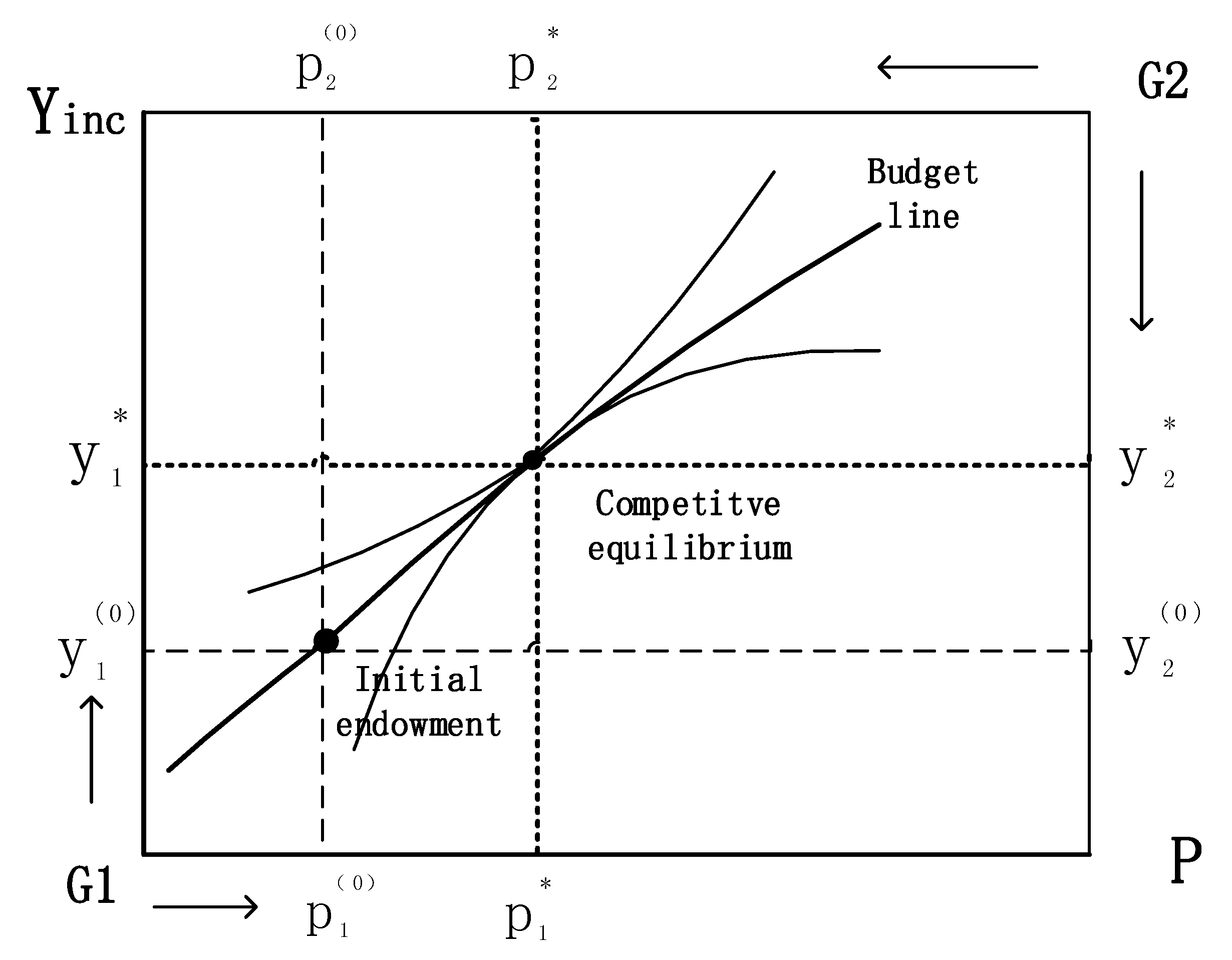
We analyze the consumption choice behaviors of G1 and G2 using the Edgeworth box, as shown in Figure 3.

Since the budget line slope of G1 and G2 is w, in the Edgeworth box, $\Delta {\mathrm{y}}_2=-\Delta {\mathrm{y}}_1$, $\Delta {\mathrm{p}}_2=-\Delta {\mathrm{p}}_1$. In addition, the budget lines of G1 and G2 overlap, both passing through the initial endowment point. It is not difficult to prove that in a fully competitive market, market clearance and competitive equilibrium $\left({\mathrm{y}}_1^{\ast },{\mathrm{p}}_1^{\ast };{\mathrm{y}}_2^{\ast },{\mathrm{p}}_2^{\ast }\right)$ can be achieved through price adjustment. Moreover, the allocation of competitive equilibrium is Pareto efficient. The indifference curves of G1 and G2 are tangent under the configuration of competitive equilibrium, satisfying Equation (5):

$${\mathrm{MRS}}_1={\mathrm{MRS}}_2=\mathrm{w}.$$

(5)

2.3.2. General Equilibrium Model Constrained by the Relationship between Economy and Environment

As mentioned above, the relationship between economic output and environmental pollution is $F\left(Y_{out},P\right)=0$. The total economic output of a society is equal to the total economic income, satisfying ${\mathrm{Y}}_{out}={\mathrm{Y}}_{inc}$, denoted as Y. Hence, $F\left(Y,P\right)=0$ constitutes the constraint condition of economic income and environmental pollution distribution. Apparently, $\mathrm{Y}={\mathrm{y}}_1+{\mathrm{y}}_2$, $\mathrm{P}={\mathrm{p}}_1+{\mathrm{p}}_2$.

For any given total consumption bundle $\left(Y,P\right)$ on the $F\left(Y,P\right)=0$ curve, we can draw the corresponding Edgeworth box. Therefore, the general equilibrium model is obtained under the constraint of the relationship between economy and environment, as shown in Figure 4.

In the Edgeworth box, the tangent points of G1 and G2 indifference curves constitute the Pareto set. Each consumption bundle in the set is Pareto efficient, and in these Pareto-efficient consumption bundles, each slope (MPV) of the marginal rate of substitution of MRS and $F\left(Y,P\right)=0$ is equal, that is:

$${\mathrm{MRS}}_1={\mathrm{MRS}}_2=\mathrm{MPV}.$$

(6)

2.4. Introduction of the Theoretical Model of Environmental Justice

If we use ${\mathsf{\theta }}_1={\mathrm{y}}_1/\mathrm{Y}$ and ${\mathsf{\theta }}_2={\mathrm{y}}_2/\mathrm{Y}$ to represent the economic revenue share of G1 and G2, respectively, it satisfies ${\mathsf{\theta }}_1+{\mathsf{\theta }}_2=1$; if we use ${\mathsf{\gamma }}_1={\mathrm{p}}_1/\mathrm{P}$ and ${\mathsf{\gamma }}_2={\mathrm{p}}_2/\mathrm{P}$ to represent the share of environmental pollution borne by G1 and G2, respectively, it satisfies ${\mathsf{\gamma }}_1+{\mathsf{\gamma }}_2=1$. Then, we can introduce the concept of “environmental justice”: the share of environmental pollution borne by each group is equal to its share of economic income. That is, when any group occupies a certain share of economic income, it should also bear the same share of environmental pollution. Based on this definition, environmental justice can be denoted as Equation (7):

$${\mathsf{\theta }}_1={\mathsf{\gamma }}_1,{\mathsf{\theta }}_2={\mathsf{\gamma }}_2.$$

(7)

If ${\mathsf{\theta }}_1>{\mathsf{\gamma }}_1,{\mathsf{\theta }}_2<{\mathsf{\gamma }}_2$, G1 transfers part of the cost of environmental pollution to G2; if ${\mathsf{\theta }}_1<{\mathsf{\gamma }}_1,{\mathsf{\theta }}_2>{\mathsf{\gamma }}_2$, G2 transfers part of the cost of environmental pollution to G1; both relations present environmentally inequality.

We add environmental justice considerations to the general equilibrium model shown in Figure 4. As shown in Figure 5, for any given total consumption bundle on the curve $F\left(Y,P\right)=0$, we can confirm an environmental justice line, that is, line OA. If and only if the distribution of economic income and environmental pollution realizes the allocation on line OA can environmental justice be realized. For the allocation below line OA, G1 bears the cost of environmental inequality; for the allocation above line OA, G2 bears the cost of environmental inequality. Considering that the competitive equilibrium can appear only on the Pareto set, if and only if the distribution of economic income and environmental pollution exactly realizes the allocation of the intersection point J of the Pareto set and environmental justice line can Pareto-efficient market equilibrium and environmental justice be achieved simultaneously.

In a fully competitive market, on the premise of ensuring Pareto efficiency, for any given total consumption bundle $\left(Y,P\right)$ on the curve $F\left(Y,P\right)=0$, there is only one equilibrium configuration that can realize environmental justice. Thus, there is little chance of realizing environmental justice, for it is realized only when the initial endowment is under a particular configuration. This indicates that environmental injustice is normal in competitive markets.

Therefore, the empirical research of this paper focuses on determining the population, economic, and social characteristics of environmentally vulnerable groups to make targeted use of the “visible hand” to promote environmental justice.

3. Methodology for Investigating Environmental Inequality in China

3.1. Econometric Models

There are two main empirical research purposes in this paper. First, the study focuses on what kinds of demographic and socioeconomic characteristics are associated with the distribution of industrial pollution sources in the four economic zones and whether there are disproportionate environmental effects for special groups. Second, a comparative analysis is carried out for the special groups in different economic zones to examine whether there are significant heterogeneities in environmental inequality among the economic zones.

To achieve the first research objective mentioned above, specific econometric models are constructed according to the general form of China’s environmental justice research model [25] as follows:

$$\begin{array}{c}{P}_i={\beta }_0+{\beta }_{1}mino{r}_i+{\beta }_{2}sin{c}_i+{\beta }_{3}urba{n}_i+{\beta }_{4}migran{t}_i+{\beta }_{5}r{2}_i+{\beta }_{6}r{3}_i+{\beta }_{7}r{4}_i+\\ X_i^{\prime }\delta +{\epsilon }_i,\end{array}$$

(8)

where i is the geographical unit at the county level. Explained variable $P_i$ represents the number of industrial pollution sources in county i. Regarding the independent variables, $mino{r}_i$ represents the proportion of minority population, $sin{c}_i$ represents the income level, $urba{n}_i$ represents the urbanization rate, and $migran{t}_i$ represents the migrant population index. $r{2}_i$, $r{3}_i$, and $r{4}_i$ are dummy variables indicating whether county i belongs to the Beijing–Tianjin–Hebei economic zone, the Chengdu–Chongqing economic zone, or the Pearl River Delta economic zone, respectively. Since the Yangtze River Delta economic zone ranks first among the four economic zones in terms of its per capita income level, it is set as the benchmark group with dummy variable $r{1}_i$ which is not introduced in the above Equation. $X_i$ is the column vector of other explanatory variables in the model, including $Ln{(psize)}_i$, $gende{r}_i$, $youn{g}_i$, $midsc{h}_i$, and $une{m}_i$. They refer to population size, sex ratio, age structure, education level, and unemployment rate, respectively. ${\beta }_0$, ${\beta }_1$, ${\beta }_2$, ${\beta }_3$, ${\beta }_4$, ${\beta }_5$, ${\beta }_6$, and $\delta$ are the parameters to be estimated, ${\epsilon }_i$ is the random error. The detailed variable definitions, explanations, and corresponding data sources are listed in Table S1 of Supplementary Materials.

Considering the obvious heterogeneity in the development of the regions where there are net population outflows and inflow, we divide the status of migrant population ${\mathrm{migrant}}_{\mathrm{i}}$ into three gradients for investigation, which are represented by $netmi{g}_i$, $mi{g}_i$, and $rmi{g}_i$. Among them, $netmi{g}_i$ is the ratio of the permanent resident population to the registered population, which represents the net population flow; $mi{g}_i$ and $rmi{g}_i$ are the percentages of migrants and rural migrants relative to the permanent resident population, respectively (see the details in Table S1). Thus, three benchmark models are constituted, as shown in Equations (9)–(11):

$$\begin{array}{c}{P}_i={\beta }_0+{\beta }_{1}mino{r}_i+{\beta }_{2}sin{c}_i+{\beta }_{3}urba{n}_i+{\beta }_{4}netmi{g}_i+{\beta }_{5}r{2}_i+{\beta }_{6}r{3}_i+{\beta }_{7}r{4}_i+\\ X_i^{\prime }\delta +{\epsilon }_i,\end{array}$$

(9)

$$\begin{array}{l}{P}_i={\beta }_0+{\beta }_{1}mino{r}_i+{\beta }_{2}sin{c}_i+{\beta }_{3}urba{n}_i+{\beta }_{4}mi{g}_i+{\beta }_{5}r{2}_i+{\beta }_{6}r{3}_i+{\beta }_{7}r{4}_i+X_i^{\prime }\delta \\ +{\epsilon }_i,\end{array}$$

(10)

$$\begin{array}{c}{P}_i={\beta }_0+{\beta }_{1}mino{r}_i+{\beta }_{2}sin{c}_i+{\beta }_{3}urba{n}_i+{\beta }_{4}rmi{g}_i+{\beta }_{5}r{2}_i+{\beta }_{6}r{3}_i+{\beta }_{7}r{4}_i+\\ X_i^{\prime }\delta +{\epsilon }_i.\end{array}$$

(11)

Furthermore, to study whether there is heterogeneity in environmental inequality for specific groups from the four economic zones, we introduce the cross term of six variables, that is, race and income indicators ($mino{r}_i$ and $sin{c}_i$) following US principles, urbanization ($urba{n}_i$), and migrants status ($netmi{g}_i$, $mi{g}_i$, and $rmi{g}_i$) in the Chinese context, replacing the original variable in the benchmark model with the dummy variables for different economic zones one at a time. Then, we can obtain the corresponding extended models. Taking the comparison of environmental inequality among the economic zones based on the ethnic perspective as an example, the extended models are shown as Equations (12)–(14):

$$\begin{array}{ll}{P}_i=& {\beta }_0+{\beta }_{1}r{1}_i\times mino{r}_i+{\beta }_{2}r{2}_i\times mino{r}_i+{\beta }_{3}r{3}_i\times mino{r}_i+{\beta }_{4}r{4}_i\times mino{r}_i+\\ & {\beta }_{5}sin{c}_i+{\beta }_{6}urba{n}_i+{\beta }_{7}netmi{g}_i+{\beta }_{8}r{2}_i+{\beta }_{9}r{3}_i+{\beta }_{10}r{4}_i+X_i^{\prime }\delta +{\epsilon }_i,\end{array}$$

(12)

$$\begin{array}{l}{P}_i={\beta }_0+{\beta }_{1}r{1}_i\times mino{r}_i+{\beta }_{2}r{2}_i\times mino{r}_i+{\beta }_{3}r{3}_i\times mino{r}_i+{\beta }_{4}r{4}_i\times mino{r}_i\\ +{\beta }_{5}sin{c}_i+{\beta }_{6}urba{n}_i+{\beta }_{7}mi{g}_i+{\beta }_{8}r{2}_i+{\beta }_{9}r{3}_i+{\beta }_{10}r{4}_i+X_i^{\prime }\delta \\ +{\epsilon }_i,\end{array}$$

(13)

$$\begin{array}{l}{P}_i={\beta }_0+{\beta }_{1}r{1}_i\times mino{r}_i+{\beta }_{2}r{2}_i\times mino{r}_i+{\beta }_{3}r{3}_i\times mino{r}_i+{\beta }_{4}r{4}_i\times mino{r}_i\\ +{\beta }_{5}sin{c}_i+{\beta }_{6}urba{n}_i+{\beta }_{7}rmi{g}_i+{\beta }_{8}r{2}_i+{\beta }_{9}r{3}_i+{\beta }_{10}r{4}_i+X_i^{\prime }\delta \\ +{\epsilon }_i.\end{array}$$

(14)

3.2. Dataset and Estimation

Aiming at the comparative study of environmental inequality among the four economic zones, we adopt a unit-based analysis with the county as the geographical unit. This includes 117 counties of the Yangtze River Delta, 151 counties of Beijing–Tianjin–Hebei, 123 counties of Chengdu–Chongqing, and 53 counties of the Pearl River Delta, with a total of 444 geographical units (China’s environmental problems have originated from the process of industrialization, which has mainly spread from sparsely distributed cities to the surrounding areas. This process thus formed an industrial economic belt with distinct regional characteristics, which mainly includes the four economic zones that have been regarded not only as the four growth poles of China’s economy during the past decades but also as regions with more prominent environmental problems. In addition, the number of selected counties, 444, is the maximum sample size that can be obtained from both environmental and demo-socioeconomic aspects within the four economic zones). The county administrative regions are chosen as the geographical units for the following reasons: (1) The demographic and socioeconomic data of the geographical units below the county level (i.e., the township, town, street, or village level) in the four major economic zones cannot be obtained from public sources. For example, only some of the township and street data in the Pearl River Delta region are available according to the 2010 population census, making the county level the smallest geographical unit whose analysis is statistically feasible. (2) The prefecture-level geographical unit [25] cannot meet the measurement requirements for the comparative analysis of the four economic zones. For example, the Pearl River Delta region covers only 9 cities, and more than 10 independent variables are examined. We obtain data concerning the pollution of wastewater, waste gas, and sewage treatment from the MEP, shown in

Table 1. Number of state-controlled industrial pollution sources in the studied economic zones.

Dummy	Economic Zones	Total Pollution Sources	Wastewater	Waste Gas	Sewage Treatment
r1	Yangtze River Delta	869	236	425	245
r2	Beijing–Tianjin–Hebei	576	202	288	124
r3	Chengdu–Chongqing	488	171	239	118
r4	Pearl River Delta	210	57	64	101
-	Sum of the four zones	2143	666	1016	588

Note: As to the Total Pollution Sources, duplicates of pollution sources that have been listed on the state control list several times due to different monitoring types have been deducted.

.

The population, social, and economic variables at the county level in 2010 are mainly collected from prefecture-level census data in the 2010 population census, the statistical yearbooks for 2011 of each city, and the statistical bulletin on the economic and social development of each county in 2010. The main statistics of the independent variables associated with the benchmark model are shown in Table S2.

In addition, there may be endogeneity problems when there is reverse causality between the industrial pollution source enterprises and the independent variables, e.g., income level. We will show the results of Ordinary Least Squares (OLS) estimation and the estimations based on Two-Stage Least Squares (2SLS) with instrumental variables. The principal component score of the current period income will be taken as the instrumental variables instrumented with first-and second-order lags of income score or first- and second-order lags of the combination of the per capita disposable income of urban residents and the per capita net income of rural households. The results of overidentifying restrictions of instrumental variables and the Hausman specification test are both shown in the results tables. Moreover, with regard to concerns about possible multicollinearity, we calculate the variance inflation factor (VIF) of the model, according to which the independent variable VIF scores and the mean VIFs of most models are no greater than 10. For some models whose mean VIFs are greater than 10, the VIF scores of the respective variables are observed to be mainly caused by the introduction of cross terms. Therefore, on the premise of not affecting the validity of the estimation results, we conduct the regression after decentralizing some cross terms and replacing the original indicators. Thus, the possibility of multicollinearity in the model is greatly decreased, which indicates that major multicollinearity issues are not present in our models on the whole.

4. Results of Baseline Models

This section takes the counties in the four economic zones as geographic units to answer the key question of whether environmental inequality occurs in the distribution of state-controlled industrial pollution sources. The estimation results for the overall industrial pollution sources in the baseline model (9)–(11) are shown in

Table 2. Results of four major economic zones based on the baseline model.

	Regression Model	Overall Industrial Pollution Sources
		(1)	(2)	(3)	(4)	(5)	(6)
Variables		OLS			2SLS
lpsize		2.379 ***	2.356 ***	2.341 ***	2.302 ***	2.284 ***	2.274 ***
		(0.353)	(0.357)	(0.342)	(0.337)	(0.343)	(0.326)
gender		0.0122 *	0.0137 *	0.0137 **	0.0132 *	0.0149 **	0.0144 **
		(0.00695)	(0.00712)	(0.00603)	(0.00690)	(0.00717)	(0.00606)
young		0.0553	0.0256	−0.0361	0.0270	0.0101	−0.0590
		(0.0650)	(0.0636)	(0.0585)	(0.0660)	(0.0653)	(0.0610)
midsch		0.133 ***	0.124 ***	0.107 ***	0.136 ***	0.127 ***	0.110***
		(0.0358)	(0.0355)	(0.0335)	(0.0362)	(0.0358)	(0.0338)
unem		0.112	0.146	0.159	0.110	0.150	0.156
		(0.172)	(0.177)	(0.163)	(0.169)	(0.173)	(0.160)
minor		0.00717	0.00472	−0.000642	0.00857	0.00676	0.000789
		(0.0182)	(0.0180)	(0.0183)	(0.0178)	(0.0177)	(0.0180)
sinc		0.142	0.166	0.142	0.452	0.487	0.418
		(0.291)	(0.308)	(0.291)	(0.333)	(0.348)	(0.332)
urban		−0.0352 **	−0.0357 **	−0.0392 **	−0.0381 **	−0.0379 **	−0.0417 ***
		(0.0162)	(0.0161)	(0.0158)	(0.0164)	(0.0162)	(0.0160)
netmig		−0.429 *			−0.408 *
		(0.248)			(0.237)
mig			−0.00344			−0.00929
			(0.0252)			(0.0244)
rmig				0.0494			0.0487
				(0.0380)			(0.0373)
region2		−3.382 ***	−3.342 ***	−3.154 ***	−2.968 ***	−2.969 ***	−2.790 **
		(1.173)	(1.184)	(1.213)	(1.131)	(1.147)	(1.168)
region3		−2.760 **	−2.869 **	−3.068 ***	−2.280 **	−2.387 **	−2.633 **
		(1.203)	(1.197)	(1.148)	(1.158)	(1.146)	(1.085)
region4		−4.314 ***	−4.473 ***	−5.023 ***	−4.111 ***	−4.246 ***	−4.827 ***
		(1.232)	(1.226)	(1.199)	(1.192)	(1.181)	(1.151)
Constant		−34.57 ***	−32.25 ***	−27.20 ***	−31.93 ***	−30.50 ***	−25.03 ***
		(6.576)	(6.567)	(6.129)	(6.314)	(6.442)	(5.964)
VIF		2.25	2.67	2.29
Overidentify					0.1176	0.1082	0.1646
Hausman					0.0066	0.0081	0.0166
Observations		444	444	444	444	444	444
R-squared		0.150	0.149	0.153	0.149	0.148	0.152

Note: Heteroscedasticity-robust standard errors are in parentheses. The estimation results in the first, second, and third columns correspond to $netmi{g}_i$, $mi{g}_i,$ and $rmi{g}_i$ in the baseline model (Equations (9) and (10)), respectively. The same applies to all tables hereafter. *** p < 0.01, ** p < 0.05, * p < 0.1.

. Since the Hausman test rejects the null hypothesis of exogenous model variables at the significance level of 1%, the analysis in this part is based on the 2SLS estimation results.

First, according to the results of the basic demographic and socioeconomic indicators, population size $Ln{(psize)}_i$ and education level $midsc{h}_i$ were significantly positive. For each 1% increase in the size of the population, there will be 2 to 3 more sources of pollution controlled by the state. For every 10% increase in the proportion of the population with secondary education, there will be 1 to 2 more sources of industrial pollution. In addition, neither age structure $youn{g}_i$ nor unemployment level $une{m}_i$ constitute significant factors affecting the unequal distribution of industrial pollution sources. It is worth noting that the results of the gender ratio in the samples of the four economic zones at the county level are different from those in the nationwide samples of the prefecture level in He et al. [25], all of which are significantly positive at the significance level of 10%. This finding indicates that in the four major economic zones, men are more exposed to environmental risks caused by industrial pollution than women, and every doubling of the male population compared with the female population corresponds to an additional 1 to 2 countries controlling industrial pollution sources.

In particular, in the four economic zones, the proportion of the minority population and income level do not constitute significant factors affecting the number of state-controlled pollution sources. Although the coefficients of $mino{r}_i$ and $sin{c}_i$ are both positive, they are not statistically significant at the level of 10%. On the one hand, except for Chengdu–Chongqing, the four economic zones are not main settlements and autonomous areas of ethnic minorities. The mean value and standard deviation of ethnic minorities in the county samples are only 3.831% and 11.42, respectively, which vary greatly to 15.92% and 26.46 for prefectures nationwide. Ethnic minorities are more evenly dispersed in the four economic zones, which makes the environmental inequality for ethnic minorities observed at the geographical unit of the county nonsignificant. On the other hand, as the “four poles” of China’s rapid economic growth, the four economic zones have higher development levels than the national average. Among them, the Yangtze River Delta, Beijing–Tianjin–Hebei, and Pearl River Delta are the three major city clusters in the eastern coastal region, and Chengdu–Chongqing is a strategic highland of economic development in the western region. In this context, these four economic zones have become the preferred areas for the Chinese middle class to live and work. Especially in the Yangtze River Delta and the Pearl River Delta, the progress of deindustrialization in recent years makes the relationship between income level and the number of industrial pollution sources appear significantly different from that suggested by national-level characteristics.

First, from the perspective of China’s characteristics, the urbanization rate shows a consistent and significantly negative result, indicating that among the four major economic zones, residents living in the counties with lower urbanization levels are exposed to a higher level of industrial pollution, and vice versa. On the one hand, this result proves that most regions of the four major economic zones are experiencing urbanization and deindustrialization. On the other hand, this suggests that at a higher level of economic development, there is inequality in the distribution of industrial pollution between urban residents and rural residents, with the latter suffering more negative externalities. Second, counties with net outflow of the population suffer higher industrial pollution than those with net inflow, which is consistent with the results at the prefectural level [25]. However, migrant workers are more likely to be exposed to industrial pollution in the four economic zones, although this result is not statistically significant. Finally, concerning the dummy variables of the four economic zones, significantly fewer state-controlled pollution sources are controlled in Beijing–Tianjin–Hebei, Chengdu–Chongqing, and Pearl River Delta than in the Yangtze River Delta. As the Yangtze River Delta is an irreplaceable “leader” of China’s economic development, the results indicate that there is no obvious regional environmental inequality among the four economic zones.

5. Comparative Study Based on Extended Models

This part investigates the differences in the demographic and socioeconomic characteristics between the US and the Chinese contexts in terms of the environmental inequality of the allocation of state-controlled industrial pollution sources, considering waste gas and wastewater, in the four economic zones. For the convenience of comparison and because of space limitation, only the estimation results of the relevant cross terms and some important parameters in the model are listed here. The full set of estimation results can be found in the supplementary materials online.

5.1. Comparative Analysis of Ethnic Groups

First, for the environmental distribution of ethnic minorities in different economic zones based on the principle of environmental justice in the US, we add the estimation results of the cross term of $mino{r}_i$ and the dummy variables for economic zones, as shown in

Table 3. Results of environmental inequality based on ethnicity.

Waste Gas
	Regression Model	OLS			2SLS
Variables		(1)	(2)	(3)	(4)	(5)	(6)
r1 × minor		−0.255	−0.211	−0.261	−0.261 *	−0.213	−0.266 *
		(0.162)	(0.164)	(0.162)	(0.158)	(0.159)	(0.158)
r2 × minor		−0.00683	−0.00708	−0.00679	−0.00570	−0.00587	−0.00571
		(0.00628)	(0.00644)	(0.00630)	(0.00617)	(0.00635)	(0.00618)
r3 × minor		−0.00987 *	−0.00877	−0.0114 **	−0.0102 *	−0.00890	−0.0117 **
		(0.00596)	(0.00601)	(0.00577)	(0.00580)	(0.00585)	(0.00562)
r4 × minor		0.314 **	0.275 *	0.190	0.318 ***	0.290 *	0.197
		(0.126)	(0.155)	(0.157)	(0.123)	(0.149)	(0.151)
VIF		2.68	2.96	2.61
Overidentify					0.299	0.2938	0.2086
Hausman					0.0006	0.0005	0.0016
Observations		444	444	444	444	444	444
R-squared		0.094	0.097	0.091	0.093	0.096	0.090
Wastewater
	Regression Model	OLS			2SLS
Variables		(7)	(8)	(9)	(10)	(11)	(12)
r1 × minor		0.964	1.034	0.963	0.955	1.031	0.954
		(1.252)	(1.289)	(1.249)	(1.226)	(1.263)	(1.222)
r2 × minor		−0.00459	−0.00504	−0.00349	−0.00286	−0.00322	−0.00166
		(0.00982)	(0.0100)	(0.00999)	(0.00956)	(0.00979)	(0.00979)
r3 × minor		0.0277	0.0289	0.0276	0.0272	0.0287	0.0271
		(0.0337)	(0.0332)	(0.0335)	(0.0331)	(0.0326)	(0.0329)
r4 × minor		0.440	0.325	0.317	0.445*	0.347	0.329
		(0.270)	(0.325)	(0.356)	(0.262)	(0.319)	(0.348)
VIF		2.68	2.96	2.61
Overidentify					0.5526	0.5114	0.4277
Hausman					0.0318	0.037	0.0479
Observations		444	444	444	444	444	444
R-squared		0.080	0.081	0.080	0.080	0.080	0.079

Note: Heteroscedasticity-robust standard errors are in parentheses. *** p < 0.01, ** p < 0.05, * p < 0.1.

.

From the perspective of classified pollution sources on the distribution of waste gas sources, regressions (1)–(6) in Table 3 show a significantly positive relationship between ethnic minorities and waste gas pollution sources only in the Pearl River Delta region in most regressions, and the coefficients of the other three economic zones are negative, indicating inequality in waste gas pollution for the ethnic minorities in the Pearl River Delta region compared with the other three economic zones. This may be related to the employment situation in the Pearl River Delta after the financial crisis, when many enterprises went bankrupt. At this time, migrant workers in the Pearl River Delta returned to their hometowns for employment and entrepreneurship. In particular, the increase in migrant workers in Jiangxi, Hunan, and other nonminority provinces adjacent to the Pearl River Delta slowed or even decreased. However, as the economy recovers, industrial enterprises in the Pearl River Delta have attracted laborers from western provinces, such as Guizhou, Yunnan, and Sichuan, which are often inhabited by ethnic minorities. Therefore, ethnic minorities are increasingly recruited by industrial enterprises in the Pearl River Delta and thus are exposed to more industrial pollution sources.

The ethnic minorities in Chengdu–Chongqing have a lower level of exposure to waste gas pollution. Concerning the distribution of wastewater pollution enterprises, significant ethnically-based inequality does not occur in the four major economic zones.

5.2. Comparative Analysis of Income Level

The estimation results of the model that introduces the cross term of income level and economic zone dummy variables are listed in

Table 4. Results based on income level.

Waste Gas
	Regression Model	OLS			2SLS
Variables		(1)	(2)	(3)	(4)	(5)	(6)
r1 × sinc		0.0397	0.118	0.0484	−0.0248	0.0576	−0.0190
		(0.244)	(0.248)	(0.245)	(0.235)	(0.241)	(0.235)
r2 × sinc		0.0524	0.0960	0.0622	0.0417	0.0980	0.0488
		(0.135)	(0.135)	(0.133)	(0.155)	(0.156)	(0.152)
r3 × sinc		−0.419	−0.330	−0.366	−0.660 **	−0.581 **	−0.601 **
		(0.303)	(0.290)	(0.292)	(0.307)	(0.293)	(0.295)
r4 × sinc		0.0998	0.161	0.0745	0.155	0.198	0.102
		(0.203)	(0.214)	(0.205)	(0.236)	(0.247)	(0.238)
VIF		2.68	3.00	2.69
Overidentify					0.5835	0.5752	0.5716
Hausman					0.0975	0.0446	0.118
Observations		444	444	444	444	444	444
R-squared		0.088	0.092	0.086	0.087	0.091	0.085
Wastewater
	Regression Model	OLS			2SLS
Variables		(7)	(8)	(9)	(10)	(11)	(12)
r1 × sinc		−0.0417	0.0514	−0.0451	0.0753	0.176	0.0816
		(0.435)	(0.449)	(0.432)	(0.442)	(0.460)	(0.443)
r2 × sinc		−0.0600	−0.00296	−0.0387	−0.171	−0.100	−0.140
		(0.184)	(0.191)	(0.185)	(0.183)	(0.197)	(0.192)
r3 × sinc		0.203	0.350	0.294	−0.343	−0.198	−0.249
		(0.434)	(0.433)	(0.418)	(0.467)	(0.462)	(0.444)
r4 × sinc		0.0359	0.0803	0.0968	0.0819	0.0842	0.0943
		(0.255)	(0.288)	(0.319)	(0.279)	(0.321)	(0.354)
VIF		2.68	3.00	2.69
Overidentify					0.3336	0.326	0.3281
Hausman					0.0027	0.003	0.0041
Observations		444	444	444	444	444	444
R-squared		0.066	0.066	0.067	0.065	0.065	0.066

Note: Heteroscedasticity-robust standard errors are in parentheses. *** p < 0.01, ** p < 0.05, * p < 0.1.

. Most income indicators have no statistically significant relationship with the number of waste gas or wastewater sources, which is relevant to the economic zones considered in this paper. The Yangtze River Delta, Chengdu–Chongqing, Beijing–Tianjin–Hebei, and Pearl River Delta are four major growth poles and important urban agglomerations of China’s economy. They are the most relatively developed economic areas nationwide and are the preferred areas for the Chinese middle class to live and work. The long-term industrialization and the recent progress of deindustrialization under the supply-side structural reform cause the nonsignificant correlation between income level and the number of industrial pollution sources.

However, the results of regressions (4)–(6) show that the coefficient of $r3\times sin{c}_i$ is significantly negative, indicating that in Chengdu–Chongqing, the poorer counties have more industrial sources of waste gas, which indicates significant environmental inequality based on income level.

5.3. Comparative Analysis of Urbanization Level

In the analysis based on the total sampled counties in Table 2, the urbanization level has a significantly negative relationship with the number of industrial pollution sources in the four major economic zones. However, the estimation results in

Table 5. Results based on urbanization level.

Waste Gas
	Regression Model	OLS			2SLS
Variables		(1)	(2)	(3)	(4)	(5)	(6)
r1 × urban		−0.0212 **	−0.0190 **	−0.0218 **	−0.0230 **	−0.0207 **	−0.0235 **
		(0.00965)	(0.00954)	(0.00980)	(0.00967)	(0.00955)	(0.00979)
r2 × urban		−0.000908	0.00173	−0.00160	−0.00167	0.00123	−0.00229
		(0.00944)	(0.00944)	(0.00948)	(0.00928)	(0.00930)	(0.00932)
r3 × urban		−0.00365	−0.00165	−0.00307	−0.00377	−0.00170	−0.00322
		(0.0109)	(0.0110)	(0.0110)	(0.0107)	(0.0108)	(0.0108)
r4 × urban		0.00959	0.00932	0.00477	0.00800	0.00832	0.00357
		(0.0115)	(0.0109)	(0.0120)	(0.0114)	(0.0108)	(0.0118)
VIF		2.68	2.96	2.61
Overidentify					0.299	0.2938	0.2086
Hausman					0.0006	0.0005	0.0016
Observations		444	444	444	444	444	444
R-squared		0.093	0.097	0.091	0.092	0.096	0.091
Wastewater
	Regression Model	OLS			2SLS
Variables		(7)	(8)	(9)	(10)	(11)	(12)
r1urban		−0.0371	−0.0354	−0.0364	−0.0397	−0.0377	−0.0391
		(0.0269)	(0.0263)	(0.0256)	(0.0270)	(0.0264)	(0.0259)
r2urban		−0.0135	−0.0114	−0.0128	−0.0146	−0.0121	−0.0139
		(0.0136)	(0.0133)	(0.0129)	(0.0134)	(0.0131)	(0.0127)
r3urban		−0.00120	0.00126	0.000104	−0.00137	0.00119	−0.000133
		(0.00861)	(0.00864)	(0.00857)	(0.00849)	(0.00851)	(0.00846)
r4urban		−0.0107	−0.0150	−0.0118	−0.0130	−0.0164	−0.0137
		(0.0176)	(0.0174)	(0.0189)	(0.0173)	(0.0172)	(0.0185)
VIF		7.44	7.60	7.31
Overidentify					0.3306	0.3243	0.2905
Hausman					0.0312	0.0279	0.0383
Observations		444	444	444	444	444	444
R-squared		0.069	0.070	0.070	0.069	0.069	0.070

Note: Heteroscedasticity-robust standard errors are in parentheses. *** p < 0.01, ** p < 0.05, * p < 0.1.

show that urbanization level has different effects on the distribution of pollution sources.

First, the major finding is that the coefficient of $r1\times urba{n}_i$ in the Yangtze River Delta region has a persistently and significantly negative relationship with the number of waste gas pollution sources, indicating a disproportionate environmental risk for counties with a higher percentage of rural residents. As one of the most economically developed urban agglomerations in China, the urbanization level of the Yangtze River Delta region reaches 70.20%, on average, while the urbanization levels of Beijing–Tianjin–Hebei and Chengdu–Chongqing are 53.73% and 47.91%, respectively, for the sample year. In the Pearl River Delta region, which also has an urbanization rate of more than 70%, there is no statistically significant relationship between the urbanization rate and the number of pollution sources. There are several possible explanations for the negative correlation between urbanization level and the number of gas pollution sources in the Yangtze River Delta region. First, the urbanization model of the Yangtze River Delta region is “cleaner” in terms of economic development mode than that of the other economic zones. Second, the Yangtze River Delta economic zone has entered the developmental stage where urbanization and deindustrialization coexist. The third possibility is that the counties with high urbanization levels in the Yangtze River Delta region take advantage of their development degree to transfer polluting industries to the counties with low urbanization levels, leaving the latter exposed to higher levels of industrial pollution.

5.4. Comparative Analysis of Migrant Population

Based on the county samples of the four major economic zones, as shown in

Table 6. Results based on migrant population.

Pollution Types		Waste Gas		Wastewater
	Regression Model	OLS	2SLS	OLS	2SLS
Variables		(1)	(2)	(3)	(4)
r1 × netmig		0.273	0.281	−0.714	−0.702
		(0.573)	(0.559)	(1.189)	(1.164)
r2 × netmig		−0.280	−0.307	−0.620	−0.659
		(0.499)	(0.498)	(0.708)	(0.707)
r3 × netmig		−2.343 ***	−2.273 ***	−0.0102	0.0950
		(0.787)	(0.775)	(1.235)	(1.225)
r4 × netmig		−0.214 **	−0.204 **	−0.299 **	−0.285 **
		(0.106)	(0.104)	(0.136)	(0.134)
VIF		8.58		8.58
Overidentify			0.2805		0.2502
Hausman			0.0008		0.0341
Observations		444	444	444	444
R-squared		0.096	0.095	0.066	0.066
	Regression Model	(5)	(6)	(7)	(8)
Variables
r1 × mig		−0.0186	−0.0211	−0.0386	−0.0420
		(0.0147)	(0.0144)	(0.0286)	(0.0282)
r2 × mig		−0.0238	−0.0253 *	−0.0228	−0.0248
		(0.0153)	(0.0151)	(0.0213)	(0.0209)
r3 × mig		−0.0413 **	−0.0422 **	0.00347	0.00212
		(0.0170)	(0.0168)	(0.0247)	(0.0244)
r4 × mig		−0.0121	−0.0138	−0.0115	−0.0140
		(0.0113)	(0.0110)	(0.0160)	(0.0155)
VIF		4.49		4.49
Overidentify			0.2517		0.2502
Hausman			0.0005		0.0316
Observations		444	444	444	444
R-squared		0.094	0.093	0.068	0.068
	Regression Model	(9)	(10)	(11)	(12)
Variables
r1 × rmig		0.00833	0.00846	−0.0534	−0.0532
		(0.0194)	(0.0190)	(0.0566)	(0.0555)
r2 × rmig		−0.00856	−0.00980	0.00155	−0.000399
		(0.0220)	(0.0217)	(0.0330)	(0.0324)
r3 × rmig		−0.0508 *	−0.0502 *	0.00522	0.00616
		(0.0276)	(0.0271)	(0.0354)	(0.0348)
r4 × rmig		0.000519	0.000369	−0.00606	−0.00629
		(0.0127)	(0.0123)	(0.0167)	(0.0161)
VIF		3.29		3.29
Overidentify			0.2154		0.2076
Hausman			0.0012		0.0489
Observations		444	444	444	444
R-squared		0.090	0.089	0.069	0.069

Note: Heteroscedasticity-robust standard errors are in parentheses. *** p < 0.01, ** p < 0.05, * p < 0.1.

, the estimation results for all the migrant indicators and waste gas in Chengdu–Chongqing and the net migrant indicator for both waste gas and wastewater in the Pearl River Delta are shown to be significantly negative, which is consistent with the results at the prefecture level in He et al. [25]. The net population inflow counties of the Pearl River Delta region have a lower level of exposure to both waste gas and wastewater pollution. This also illustrates that the emitting enterprises in these two economic zones are less concentrated in the counties where the proportions of population inflow or migrant workers are high.

The estimated results of the coefficients related to migrants in this paper are contrary to the conclusions of Ma [23] and Schoolman and Ma [24], which demands a systematic explanation. On the one hand, the migrant data used in the previous two studies were collected from China’s fifth census in 2000. At that time, the migrant population was mainly engaged in labor-intensive industries with high pollution, such as the mining and textile industry. However, our study is based on the most recent data from the sixth census in 2010. A comparison of the two censuses shows that only 22.29% of China’s migrant population was engaged in business or service industries in 2000, compared with 31.28% in 2010. In addition, China’s migrant population, especially migrant workers, is more concentrated in the construction and service industries, including catering and logistics, which are not among the industrial pollution sources sampled in this paper. According to several reports on the development of China’s migrant population (Announced by the National Health Commission of the People’s Republic of China, see details in http://www.nhc.gov.cn/wjw/index.shtml.), although the manufacturing industry has always been the industry absorbing the largest proportion of the migrant population, this proportion has been continuously decreasing in the past ten years. Taking survey data from the commission in 2013 as an example, the proportion of manufacturing employees was 33.3% in 2013, down 4.1 percentage points from 2011. On the other hand, the proportion of employment in the tertiary industry is on the rise. In 2013, the proportions of employment in the wholesale and retail industry and the accommodation and catering industry were 20.1% and 11.3%, respectively, up 2 percentage points and 1.4 percentage points over 2011. Furthermore, the reason for the change in occupational structure of the migrant population may be hidden in the continuous change in their education level. In 2000, 22.90% of the migrant population in China had only completed primary school education or below, and only 14.14% of the migrant population had a college diploma or higher. However, by 2010, the ratios changed to 19.07% and 18.92%, respectively. Even when examining only the education level of migrant workers, the proportion of migrant workers having completed primary education or below decreased from 28.83% in 2000 to 22.76% in 2010, and the proportion of migrant workers with college education or above increased from 5.72% in 2000 to 9.13% in 2010.

6. Implications and Conclusions

6.1. Policy Implications

To mitigate environmental inequality, the most fundamental method is to thoroughly solve the problem of environmental destruction and pollution. However, due to the still prominent contradiction between socioeconomic development and the environment at the current stage in China, a more realistic approach is to promote more even distribution of environmental benefits to the vulnerable groups while gradually governing environmental problems and reducing the environmental burden on vulnerable groups. Specifically, some clues for policies related to more efficient ecological management and environmental regulations have been provided here.

First, environmental resources should be developed and utilized according to the concepts of an ecological civilization and tertiarization. The counties where a large part of the environmentally vulnerable groups live, such as rural areas and peripheral areas of the economic zones, often have unique ecological advantages, including beautiful natural landscapes, unique folk customs, and pluralism of traditional culture. However, disadvantageous conditions that are present during the current stage of industrialization of civilization can be changed into advantages under the perspective of an ecological civilization, where new values can be formed and environmental resources are reassessed. With the emergence and rise of the middle class in China, which prefers that consumption patterns exhibit ecological considerations, the development and utilization of environmental resources should follow the pattern of creative industries, such as providing leisure travel with ecological experiences. This type of industry is likely to obtain higher rates of value-added benefits from environmental resources, thus making correction of environmental inequality possible via increasing compensation to environmentally vulnerable groups.

Second, the benefits of sharing should be realized by localized development of environmental resources. A large number of cases in practice show that the development of local environmental resources is dominated by external capital, which makes the incremental benefits difficult to distribute to the residents in the region, while the costs and risks are borne by the local residents. To change this dilemma, local governments should be allowed to participate in the exploitation of environmental and ecological resources in an equitable manner. This can not only provide a good environment for the benefit of the public at a low cost, but also contribute to the localization (Localization, as another trend compared to globalization, refers to any economic activities in a region or country that must be adapted to local needs for development to occur.) of the resource capitalization process. For example, an appropriate method of sustainable development is to value the elements of the local ecological environment and to form a community with shared interests consisting of local residents who can negotiate with external profit-making developers. This type of collective negotiation can guarantee that the vulnerable groups and those investing capital can equally enjoy the benefits of development of localized resources. This can help to break the attachment of the vulnerable groups, including the peripheral counties within the economic zones, to other agents, especially external capital, and completely change their environmentally vulnerable status.

Finally, the degree of organization of vulnerable groups should be improved, and they should be encouraged to form various types of cooperative organizations that can effectively alleviate the problem of environmental inequality. As mentioned, organizations of environmentally disadvantaged groups can integrate their internal resources and participate equally in market economy negotiations. In addition, organized environmentally disadvantaged groups can form social capital to reduce the transaction cost of environmental governance by connecting with the country’s hierarchical environmental protection system.

6.2. Conclusions

This study focuses on Chinese environmental justice issues, which have realistic urgency but lack theoretical foundation and empirical experience. On the basis of learning and revising the US environmental justice principle, this study has two main research contributions: construction of a general equilibrium theory model of environmental justice and a comparative study on environmental inequality in four major economic zones in China.

First, by introducing environmental justice into the general equilibrium model of the competitive market for environmental pollution, we find that only when the distribution of economic income and environmental pollution exactly realizes the allocation at the intersection of the Pareto set and the environmental justice line can we achieve the Pareto-efficient market equilibrium and environmental justice at the same time. The theoretical model proves that under the premise of ensuring Pareto efficiency, it is difficult to realize environmental justice in the competitive market; environmental injustice is the normal state.

Furthermore, we take the “four poles” of China’s economic growth, the Yangtze River Delta, Pearl River Delta, Beijing–Tianjin–Hebei, and Chengdu–Chongqing, as the research objects. Taking 444 counties of the four typical economic zones as geographical units, we investigate the environmental inequality in the samples of economically developed counties. Then, we conduct a comparative analysis of the main elements of inequality in these economic zones. Our findings include the following: (1) For the four major economic zones as a whole, a lower urbanization rate corresponds to a higher risk of exposure to industrial pollution sources faced by the county residents, which means that environmental inequality occurs between urban and rural areas, and this inequality is most significant in the Yangtze River Delta region; and (2) different economic zones show heterogeneity in the key variables; for example, ethnic minorities in the Pearl River Delta are exposed to more waste gas sources while the poor in Chengdu–Chongqing face environmental inequality in the distribution of waste gas sources.

The findings of this paper provide a useful model to support further research on environmental justice issues in China. The theoretical and empirical research on environmental justice in China is expected to be enriched and developed in the near future, providing valuable references and inspiration for the sustainable and harmonious development of China’s economy and society.