An Empirical Analysis of Bitcoin Price Jump Risk

Abstract

Given that there are both continuous and discontinuous components in the movement of asset prices, existing asset pricing models that assume only continuous price movements should be revised. In this paper, we explore the features of jumps, which are discontinuous movements, by examining Bitcoin pricing. First, we identify jumps in the Bitcoin price on a daily basis, applying a non-parametric methodology and then break down the Bitcoin total rate of return into a jump rate of return and a continuous rate of return. In our empirical analysis, price jumps turn out to be independent of volatility. Moreover, the jumps in the Bitcoin price do not appear at regular intervals; rather, they tend to be concentrated in clusters during special periods, implying that once an economic crisis occurs, the crisis will last for a long time due to contagion effects and the economy will take a considerable amount of time to recover fully. Further, the contribution of the jump rate of return to the total rate of return of the Bitcoin price is lower than the contribution of the continuous return, implying that the pursuit of sustainable returns rather than large but temporary returns will improve the total rate of return over the long term. Finally, more jumps are observed when trading volume is lower, implying that market illiquidity drives discontinuous movement in asset prices. Overall, the features of jump risk are like two sides of the same coin and jump risks are expected to have a significant effect on asset pricing, suggesting that consideration of jumps is essential for risk management as well as asset pricing.

1. Introduction

Bitcoin prices have skyrocketed in recent years as the virtual currency market has been gradually expanding. Sahoo [1] shows that Bitcoin, as digital money, is a highly volatile currency using the generalized autoregressive conditional heteroskedasticity (GARCH) model. The discontinuous movement of an asset price cannot be explained by the classic asset pricing models, which do not take the jump process into account. For instance, Merton’s model assumes that there is little probability of sudden changes in asset prices. Under these circumstances, there are many calling for the consideration of jump movements in portfolio risk management as well as in asset pricing models. Aït-Sahalia and Matthys [2] allocate assets efficiently considering jumps. Cao et al. [3] study price jumps using intraday crude oil prices and natural gas futures prices and then implement model-free tests for jump activity. They observe that jumps make up 36 and 41 percent of the realized variances of crude oil and natural gas returns, respectively.

This paper clarifies the types of jump features of the Bitcoin price based on the Jiang and Omen [4] (henceforth JO) methodology. Our first research question is whether the jumps in the Bitcoin price occur frequently when the price fluctuation is large. Our second is whether these jumps appear at regular intervals. Our third is how significantly the jump rate of return contributes to the total rate of return. Finally, our fourth research question is based on our interest in what causes the price to jump.

Our empirical results show four main features of the jump movements in the Bitcoin price. First, the price jumps turn out to be independent of its volatility and, even when price volatility is high, price jumps are not apparent. Second, price jumps do not occur periodically at regular intervals but tend to appear in a cluster. Third, we show that the contribution of the jump rate of return to the total rate of return is lower than that of the continuous rate of return. Finally, we find that the discontinuous movements in the price are caused by market illiquidity.

The remainder of this paper is as follows. Section 2 presents our literature review and Section 3 describes our data and methodology employed for identifying “significant” jumps. Section 4 discusses our empirical results and Section 5 concludes the paper.

2. Related Literature Review

Several studies suggest that asset price jumps tend to be clustered. According to the concept of jump clustering, an extreme asset price movement tends to be followed by another extreme movement, causing market-to-market contagion effects. Hanousek et al. [5] show that the differences in price jump intensity before and during a crisis are found in the individual stock markets, and during the period of financial crisis the intensity of the price jumps does not evenly increase. Fičura [6] investigates both self-exciting and cross-exciting contagion effects caused by large jumps in four major currency exchange rates. Aït-Sahalia et al. [7] show the contagion effect of jump clustering by replacing a Poisson process with a Hawkes process, suggesting that jumps temporarily increase the probability of subsequent jumps occurring from market to market. Novotný et al. [8] insist that jumps deliver tradable signals only for the euro, yen, and rand among eight currencies against the U.S. dollar.

Studies on factors that drive the price jumps have also received significant attention. There are two main explanations for the source of price jumps: news announcement and illiquidity. The first references the arrival of a news announcement. In Ross [9], the asset price fluctuations depend largely on changes in the rate of information flow. In Maheu and McCurd [10], a news surprise on expected future cash flows causes above average price fluctuations, and this phenomenon might be better demonstrated by jump processes rather than Brownian motion or normal innovations. Andersen et al. [11] also show that the jump responds to specific news, and bond markets react more strongly to macroeconomic news than equity markets and foreign exchange markets. Lahaye et al. [12] analyze how news surprises explain (co)jumps using three types of assets: stock index futures, bond futures, and exchange rates. They identify the influence of the sources of shocks, such as U.S. macroeconomic releases, including federal funds target announcements, on the size, frequency, and timing of jumps across asset classes. Lee and Mykland [13] identify jump arrival times and realized jump sizes in asset prices based on a nonparametric model and then prove that individual stock jumps are connected with prescheduled earnings announcements and other company-specific news events. The second references a lack of market liquidity. Bouchaud et al. [14] show that extreme crash situations are often associated with a liquidity crisis. Będowska and Sójka [15] find that only a small part of the jump is triggered by the information released, and most jumps are due to liquidity shocks observed in the spreads, volume, and the number of trades. In addition, Madhavan [16] points to liquidity caused by an imbalanced market microstructure as a factor causing extreme price movements.

There are also studies that show that these jumps act as risks and, thus, reduce a firm’s value. Zhou [17] includes jump risk in the default process and describes that a firm can be bankrupt in an instant due to a sudden drop in its value based on a credit model with the jump risk. Duan and Yeh [18] incorporate a jump risk factor and price the jump and volatility risks. Eraker et al. [19] indicate that estimates of jump times, jump size, and spot volatility using the S&P 500 and Nasda1 100 index returns are useful for identifying the role of these factors during periods of market recession. On the other hand, studies have shown that if a jump occurs, the enterprise’s value may increase. Black and Kim [20] show that exogenous legal shocks, such as the enactment of new laws, can increase firm market value only for large firms but not for relatively midsized firms, based on event study and instrumental variable methods, among others.

Some argue that discontinuous jumps should be taken into account in determining the asset price, and they decompose the overall asset price variability into two components, continuous price volatility and discontinuous price jumps, to realistically model asset price behavior [10]. Existing models such as the Capital Asset Pricing Model [21] are based only on the assumption of continuous price movements. Li et al. [22] propose a new model that reflects the asset price dynamics in the presence of jumps as well as liquidity risks. Broadie and Jain [23] show that the swap price with consideration of its jumps is significantly different from its price without reflecting the jumps; they insist that the jump process is needed in asset pricing models. Arshanapalli et al. [24] estimate the jump component as a risk measure using the GARCH model. Pan [25] focuses on the role of jump-risk premiums in option pricing using S&P 500 index options. This new approach can help forecast the returns of asset prices and model volatility risk premium more accurately. Yan [26] insists that expected stock return is a function of the average jump size and both have a negative relation by measuring jump size as the slope of the option-implied volatility smile. Moreover, he shows that the idiosyncratic component dominates the systematic component in explaining the return predictability of the slope by decomposing total jump size into its systematic and nonsystematic slope components. Chang et al. [27] claim that the market skewness risk premium is statistically and economically significant and cannot be explained by other common risk factors.

3. Data and Methodology

3.1. Data Description

Unlike stock markets, the Bitcoin exchanges operate 24 h a day securely on the internet through a digital ledger known as a blockchain. We use the Bitcoin price as of 9 a.m., when the rate of price change is initialized and reset, from www.fr-data.net/search. The sample period is from April 2014 to August 2018. Panel A in Table 1 shows the summary statistics for daily prices of some variables including Bitcoin, international oil, the world stock index, the U.S. dollar, and gold, all of which are expected to relate to the Bitcoin price. Bitcoin variability can be seen as significantly greater than other assets. Panel B in Table 1 also shows the correlation between different asset classes. The Bitcoin price is positively correlated with three variables, the world stock index, the international oil price, and the gold price, but not with the U.S. dollar index. In particular, the Bitcoin price has a correlation with the world stock price index of 0.82, which is relatively high compared to the other variables.

Table 1. Descriptive statistics of five time series.

	Bitcoin Price	World MSCI Index	WTI Price	Gold Price	US Dollar Index
Panel A
Mean	2461.08	1814.09	57.96	1239.20	93.68
Std.Dev	3613.26	176.24	18.44	70.68	5.66
Min	178.35	1468.90	26.21	1051.10	79.09
Max	19,394.76	2248.93	107.26	1366.33	103.30
Skew	1.93	0.71	1.23	−0.56	−1.05
Kurt	3.31	−0.65	0.76	−0.31	0.53
obs	1614	1154	1115	1148	1154
Panel B
Bitcoin price	1
World MSCI Index	0.86	1
WTI price	0.10	0.15	1
Gold price	0.41	0.42	0.34	1
US Dollar Index	−0.08	−0.02	−0.86	−0.43	1

As you can see in Figure 1, the trading cost per 1 Bitcoin rose to $1147 on 4 December from about $15 in early 2013, then plummeted to $178 on 14 January 2015, recording the worst change in history. Since then, Bitcoin has been trading at somewhat stable rates. Once again starting to rise at the end of 2016, the Bitcoin price increased exponentially and peaked at $19,394 on 16 December 2017 and since then has gone downhill.

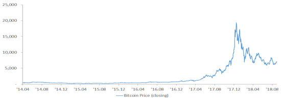
Figure 1. The time series of the Bitcoin closing price.

3.2. Methodology

This section describes the empirical methodology utilized for this study. Our jump measure is based mainly on JO’s [4] methodology and Barndorff-Nielsen and Shephard (Barndorff et al. [28,29]) (henceforth BNS) who use bipower variation (BPV) minus realized variance (RV) to test for jumps over short time intervals. Jiang and Yao [30] and Jiang and Zhu [31] use the JO methodology to describe cross-sectional stock returns. Recently, the JO measure has generated continuous follow-up research and, thus, can be meaningfully applied to the analysis of the Bitcoin price movement.

JO’s methodology starts from the point that Equation (1) below approaches the standard normal distribution under the null hypothesis that no jumps occur:

$$J{S}_0=\frac{V_{\left(0,1\right)}N}{\sqrt{{\Omega }_{SWV}}}\left(1-\frac{R{V}_N}{SW{V}_N}\right)\to \mathcal{N}\left(0,1\right),$$

(1)

where $V_{\left(0,1\right)}$ uses the BPV of BNS, and ${\Omega }_{SWV}$ (Equation (2)) shows that the following estimation method is consistent for p > 0.

$${\Omega }_{SWV}=\frac{{\mu }_6}{9}\frac{N^3{\mu }_{6/p}^{-p}}{N-p+1}{{\displaystyle \sum }}_{j=0}^{N-p}{{\displaystyle \prod }}_{k=1}^p{\left|r_{\delta ,j+k}\right|}^{6/p},$$

(2)

where ${\mu }_p=2^{p/2}\Gamma \left(\left(p+1\right)/2\right)/\sqrt{\pi }$. Therefore, by calculating the $J{S}_0$ statistic over a period of time, we statistically test whether or not a jump has occurred under the appropriate significance level. The specific algorithm for this test is as follows.

First, we calculate the ${JS}_0$ statistic using the stock return data $\left\{r_1,r_2,\dots ,r_N\right\}$ of the period to be tested, which is one day in this study. If this statistic is significant, we go to the next step. That is, if the statistic value is sufficiently extreme, the null hypothesis is rejected, implying that the jump is included during the test period. Second, for all i, ${JS}^{\left(i\right)}$ is calculated by substituting the median rate of return for the i-th rate of return. That is, $\left\{J{S}^{\left(1\right)}, J{S}^{\left(2\right)},\dots ,J{S}^{\left(N\right)}\right\}$ are recorded. Then, we calculate $J{S}_0-J{S}^{\left(i\right)}$ and record the highest return as the jump return. If when excluding the i-th rate of return, the JS statistic is the most likely to be lost, then we can assume that the i-th rate of return has contributed significantly to the rejection of the null hypothesis at the first stage. Third, we replace the recorded jump rate of return with a median rate of return, then repeat the algorithm from the first step. This process is repeated until the “no jump” null hypothesis is rejected to distinguish the jump returns.

After measuring jumps in the Bitcoin prices through the above algorithm, we calculate the jump and continuous returns of Bitcoin prices using a compounding method. The monthly jump return is calculated considering only the rate of return on the day of the jump (all the returns on the day when there is no jump are considered as zero). When calculating the continuous return, only the return on the day without the jump is taken into consideration (the return on the day of the jump is assumed to be zero). Thus, we decompose the total rate of return (TR) into the continuous rate of return (CR) and the jump rate of return (JR) on a monthly basis, and the following Equation (3) is established. Here, the contribution of the jump risk to total risk, calculated as $\mathrm{p}=\frac{Var\left(J{R}_t\right)}{Var\left(T{R}_t\right)}$, is assumed to be six.

$$\left(1+TR\right)=\left(1+CR\right)\times \left(1+JR\right)$$

(3)

Our methodology for the cluster phenomenon of jumps is based on the Pearson chi-squared test. This test helps us see whether jumps occur at regular intervals or are clustered. The Pearson chi-squared statistic $\left({\mathsf{\chi }}^2\right)$ is as follows.

$${\mathsf{\chi }}^2={\displaystyle \sum }_{month t}{\left[\frac{O_t-E_t}{\sqrt{E_t}}\right]}^2,$$

(4)

where $O_t$ is the number of jumps in month t and $E_t$ is the expected number of jumps under the assumption of the Poisson distribution, which is calculated by the total number of jumps divided by total number of months. The chi-square statistic is the test statistic that measures the difference between the distribution of the sample data and the expected Poisson distribution. The greater the difference between the observations in the sample and the expected values, the greater the chi-square statistic is and the more likely it is to reject the assumption of the Poisson distribution.

A Poisson process consists of events that occur at random times, where the interarrival times of each jump are assumed to be constant. In other words, the number of jumps is equally distributed over an equal period of time. The null hypothesis of the goodness-of-fit test for a Poisson distribution is as follows:

$$H_0:\lambda =constant \left(\mathrm{Poisson}\right)$$

(5)

where $\lambda$ indicates the interarrival times of each jump. If the interarrival times of each jump are not constant, the null hypothesis will be rejected in the Poisson distribution test, which means that the jumps are clustered.

4. Empirical Results

Here, we identify true jumps and show whether the variability in Bitcoin prices has a relationship with the jumps, whether these jumps occur at a given cycle or at a particular interval, whether the contribution of the jump rate of return to the gross rate of return is higher than the contribution of the continuous rate of return, and what drives the jumps in the Bitcoin prices.

First, the identification of the jump component depends on the significance of the algorithm. The higher the level of significance, the more frequently jumps occur. For instance, if the significance level is set at 10%, more jumps are estimated compared to 1% because the probability of being recognized as a jump increases. Under the same logic, the implication is that the jump identified at the significance level of 1% is the only true jump. Table 2 provides information on the basic statistics of the jump rate and the continuous rate of return, showing the lower the significance is, the fewer jumps there are out of the total volume of transactions. The estimated number of jump days of the total trading days is 69 days at the significance level 1%, 97 days at the significance level 5%, and 122 days at the significance level 10%. In addition, the lower the significance level is, the higher the average of the jump rate of return, the lower its standard deviation, the higher both its skewness and kurtosis, and the opposite movement for the continuous rate of returns.

Table 2. Estimates of the monthly returns of Bitcoin price.

Significance Level		Alpha = 1%	Alpha = 5%	Alpha = 10%
The number of jump days		69	97	122
Monthly CR	N	53	53	53
	Mean	0.057	0.059	0.061
	Std.Dev	0.205	0.189	0.184
	Min	−0.327	−0.185	−0.185
	Max	0.676	0.676	0.676
	Skew	1.154	1.610	1.684
	Kurt	1.793	2.925	3.397
Monthly JR	N	53	53	53
	Mean	0.017	0.015	0.014
	Std.Dev	0.097	0.123	0.137
	Min	−0.271	−0.271	−0.353
	Max	0.409	0.409	0.409
	Skew	1.093	0.534	0.070
	Kurt	6.053	1.927	1.929

Second, given the fact that a jump is a risky and unexpected big movement against volatility in the current market, our first hypothesis is that more jumps in the Bitcoin price will appear if its fluctuation is higher. However, it turns out not to be true in our empirical analysis. As Table 2 shows, at all significance levels, the standard deviation of the jump yield is lower than the standard deviation of the continuous yield. Between 2016 and 2017, the price of Bitcoin jumped more frequently, as shown in Table 3, but its volatility was lower, as shown in Panel A of Figure 2. This phenomenon implies that a large movement in price does not always result in a jump. That is, if the volatility of a certain month is large, it may not be a jump, and even if the volatility of the month is small, it may be a jump. Furthermore, given that assets with large jump risk are likely to have low volatility, it is possible to interpret that the preference for a jump occurring may increase in the process of creating an optimal portfolio [32].

Table 3. The number of jumps per year.

Year	Total Trading Day	Jump (Alpha = 1%)	Jump (Alpha = 5%)	Jump (Alpha = 10%)
Total period (2014.04–2018.08)	1614	69	97	122
2014.04–2014.12	275	6	10	10
2015	365	9	14	15
2016	366	27	28	41
2017	365	25	30	34
2018.01–2018.08	243	2	15	22

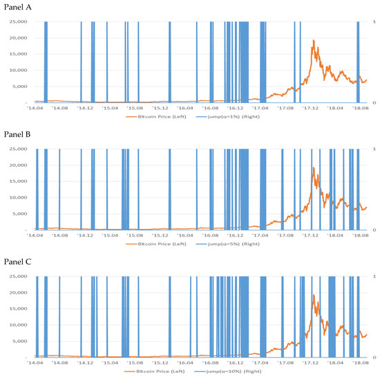
Figure 2. The jump identification.

Third, jump clustering is a theory that the jumps in asset prices are likely to persist for a while if a jump occurs once. As shown in Table 4, a test of how consistently jumps occur with Pearson chi-squared statistics shows that they are clustered regardless of significance level by rejecting the null hypothesis that the jump’s interarrival time is constant. In Figure 2, we visualize the jump intervals in a time series graph on a daily basis to see if the jumps are evenly distributed or clustered. We see that the price jumps are not evenly distributed but are in a crowd and that jump clustering is more frequently found during the second half of 2016 through the first half of 2017. This clustering phenomenon suggests that it will take considerable time for the effects to be resolved and eliminated once the economy is subjected to an extraordinary impact. This is consistent with the findings of Hanousek et al. [5] on European stock markets.

Table 4. The goodness-of-fit test for a Poisson distribution.

Significance (α)	Pearson Chi-Squared Statistics
1%	326.58
5%	268.54
10%	297.66

Fourth, we expect that the contribution of the jump return to the gross margin will be relatively higher than the continuous return contribution. However, our empirical analysis supports the contrary conclusion. The contribution of the jump rate of return is calculated by the formula of Equation (7) derived from Equations (3) and (6) on the basis of the cumulative return. As shown in Table 5, the contribution of the jump return to the total return is only around 20 to 35 percent, while the contribution of the continuous return is between 65 and 80 percent. Jump contribution to the gross yield, regardless of the significant level, seems to be negatively skewed. Figure 3 also shows that, at the significance of 1%, the number of months when the contribution of the jump rate of return to the gross rate of return exceeds the contribution of the continuous rate of return is only 13, while the contribution of the continuous return exceeds the contribution of the jump return in 40 months. To sum, unlike our expectations, the contribution of the continuous return to the total return exceeds the contribution of the jump return, implying that the pursuit of sustainable and stable returns rather than large but temporary returns, like a lottery, will help improve total returns over the long term.

$$\ln \left(1+\mathrm{cumulative} TR\right)=\ln \left(1+\mathrm{cumulative} CR\right)+\ln \left(1+\mathrm{cumulative} JR\right)$$

(6)

$$Jump contribution to total return=100\times \frac{\ln \left(1+\mathrm{cumulative} JR\right)}{\ln \left(1+\mathrm{cumulative} TR\right)}$$

(7)

Table 5. Estimates of the contribution of jump return to total return.

	Contribution of Jump Return to Total Return (%)
	Alpha = 1%	Alpha = 5%	Alpha = 10%
MEAN	20.30	31.01	34.12
Std.Dev	63.52	72.07	75.44
Min	−276.83	−276.83	−276.83
Max	248.55	248.56	248.56
Skew	−0.82	−0.71	−0.71
Kurt	11.20	6.73	5.35

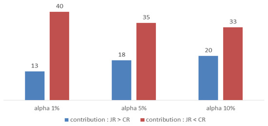
Figure 3. Comparison of contributions to total rate of return between jump rate of return and continuous rate of return. The blue bars show the number of months the contribution of the jump rate of return to the gross rate of return exceeds the contribution of the continuous rate of return, depending on the significance level. The red bars show the opposite.

Fifth, it is expected that the more active the transaction is, the more frequently the asset price will jump. However, it turns out not to be true because smaller trading volumes result in more frequent jumps, as shown in Figure 4. This suggests that the market is inefficient, namely, information asymmetry is large, which results in more frequent jumps in asset prices when the volume of transactions is sluggish. Under this logic, the existence of a jump supports that the market is inefficient. This is in contrast to Buckley et al. [33] who argue that jump risks improve market efficiency by reducing the asymmetry of information and then help optimize portfolio strategies.

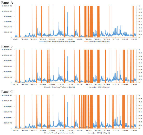
Figure 4. The jump identification of the Bitcoin price and a time series of Bitcoin trading volume depending on the significance level.

5. Conclusions

Jumps are very important in asset pricing. This article examines the distributional properties of the jumps in Bitcoin prices. First, we identify jumps in the Bitcoin price by applying the JO methodology and then break down the Bitcoin’s total rate of return into the jump rate of return and the continuous rate of return.

Our empirical results are as follows. First, the volatility of the jump return is lower than that of the continuous return, implying that a large movement in price does not always result in a jump and preference for a jump occurrence may help in constructing an optimal portfolio. Second, the jumps in the Bitcoin price are not evenly distributed but clustered, implying contagion effects of various shocks to the economy. Third, the contribution of the continuous return to the total return exceeds the contribution of the jump return, implying that a preference for sustainable and stable returns rather than for large but temporary returns can improve the total rate of return over the long term. Fourth, more jumps are observed when trading volume is lower, implying market illiquidity can trigger jumps in asset prices. Overall, the features of the jumps are like two sides of the same coin and jumps are expected to have a significant effect on asset pricing.

This paper argues that allowing for price jumps can improve the fitting for the time series of equity returns when considering the nature of such jumps. Moreover, for risk management and asset allocation, it is crucial to be able to distinguish between jumps and continuous sample path price movements because jumps offer profitable signals. In further research, a multivariate jump-driven financial asset model could be built utilizing the results of this study.

References

- Sahoo, P.K. Bitcoin as digital money: Its growth and future sustainability. Theor. Appl. Econ. 2017, 53–64. [Google Scholar]
- Aït-Sahalia, Y.; Matthys, F. Robust consumption and portfolio policies when asset prices can jump. J. Econ. Theory 2019, 179, 1–56. [Google Scholar] [CrossRef]
- Cao, W.; Guernsey, S.B.; Linn, S.C. Evidence of infinite and finite jump processes in commodity futures prices: Crude oil and natural gas. Phys. A 2018, 502, 629–641. [Google Scholar] [CrossRef]
- Jiang, G.J.; Oomen, R.C.A. Testing for jumps when asset prices are observed with noise—A “swap variance” approach. J. Econ. 2008, 144, 352–370. [Google Scholar] [CrossRef]
- Hanousek, J.; Kočenda, E.; Novotný, J. Price jumps on European stock markets. Borsa Istanb. Rev. 2014, 14, 10–22. [Google Scholar] [CrossRef]
- Fičura, M. Modelling Jump Clustering in the Four Major Foreign Exchange Rates Using High-Frequency Returns and Cross-exciting Jump Processes. Procedia Econ. Financ. 2015, 25, 208–219. [Google Scholar] [CrossRef]
- Aït-Sahalia, Y.; Laeven, R.J.A.; Pelizzon, L. Mutual excitation in Eurozone sovereign CDS. J. Econ. 2014, 183, 151–167. [Google Scholar] [CrossRef]
- Novotný, J.; Petrov, D.; Urga, G. Trading price jump clusters in foreign exchange markets. J. Financ. Mark. 2015, 24, 66–92. [Google Scholar] [CrossRef]
- Ross, S.A. Information and Volatility: The No-Arbitrage Martingale Approach to Timing and Resolution Irrelevancy. J. Financ. 1989, 44, 1–17. [Google Scholar] [CrossRef]
- Maheu, J.M.; McCurdy, T.H. News Arrival, Jump Dynamics, and Volatility Components for Individual Stock Returns. J. Financ. 2004, 59, 755–793. [Google Scholar] [CrossRef]
- Andersen, T.G.; Bollerslev, T.; Diebold, F.X.; Vega, C. Real-time price discovery in global stock, bond and foreign exchange markets. J. Int. Econ. 2007, 73, 251–277. [Google Scholar] [CrossRef]
- Lahaye, J.; Laurent, S.; Neely, C.J. Jumps, cojumps and macro announcements. J. Appl. Econ. 2011, 26, 893–921. [Google Scholar] [CrossRef]
- Lee, S.S.; Mykland, P.A. Jumps in financial markets: A new nonparametric test and jump dynamics. Rev. Financ. Stud. 2008, 21, 2535–2563. [Google Scholar] [CrossRef]
- Bouchaud, J.-P.; Kockelkoren, J.; Potters, M. Random walks, liquidity molasses and critical response in financial markets. Quant. Financ. 2006, 6, 115–123. [Google Scholar] [CrossRef]
- Będowska-Sójka, B. Liquidity Dynamics Around Jumps: The Evidence from the Warsaw Stock Exchange. Emerg. Mark. Financ. Trade 2016, 52, 2740–2755. [Google Scholar] [CrossRef]
- Madhavan, A. Market microstructure: A survey. J. Financ. Mark. 2000, 3, 205–258. [Google Scholar] [CrossRef]
- Zhou, C. The term structure of credit spreads with jump risk. J. Bank. Financ. 2001, 25, 2015–2040. [Google Scholar] [CrossRef]
- Duan, J.-C.; Yeh, C.-Y. Jump and volatility risk premiums implied by VIX. JEDC 2010, 34, 2232–2244. [Google Scholar] [CrossRef]
- Eraker, B.; Johannes, M.; Polson, N. The Impact of Jumps in Volatility and Returns. J. Financ. 2003, 58, 1269–1300. [Google Scholar] [CrossRef]
- Black, B.; Kim, W. The effect of board structure on firm value: A multiple identification strategies approach using Korean data. JFE 2012, 104, 203–226. [Google Scholar] [CrossRef]
- Sharpe, W.F. Capital asset prices: A theory of market equilibrium under conditions of risk*. J. Financ. 1964, 19, 425–442. [Google Scholar]
- Li, Z.; Zhang, W.-G.; Liu, Y.-J.; Zhang, Y. Pricing discrete barrier options under jump-diffusion model with liquidity risk. IREF 2019, 59, 347–368. [Google Scholar] [CrossRef]
- Broadie, M.; Jain, A. The effect of jumps and discrete sampling on volatility and variance swaps. IJTAF 2008, 11, 761–797. [Google Scholar] [CrossRef]
- Arshanapalli, B.; Fabozzi, F.J.; Nelson, W. The role of jump dynamics in the risk–return relationship. IRFA 2013, 29, 212–218. [Google Scholar] [CrossRef]
- Pan, J. The jump-risk premia implicit in options: Evidence from an integrated time-series study. JFE 2002, 63, 3–50. [Google Scholar] [CrossRef]
- Yan, S. Jump risk, stock returns, and slope of implied volatility smile. JFE 2011, 99, 216–233. [Google Scholar] [CrossRef]
- Chang, B.Y.; Christoffersen, P.; Jacobs, K. Market skewness risk and the cross section of stock returns. JFE 2013, 107, 46–68. [Google Scholar] [CrossRef]
- Barndorff-Nielsen, O.E.; Shephard, N. Power and Bipower Variation with Stochastic Volatility and Jumps. J. Financ. Econom. 2004, 2, 1–37. [Google Scholar] [CrossRef]
- Barndorff-Nielsen, O.E. Econometrics of Testing for Jumps in Financial Economics Using Bipower Variation. J. Financ. Econom. 2005, 4, 1–30. [Google Scholar] [CrossRef]
- Jiang, G.J.; Yao, T. Stock Price Jumps and Cross-Sectional Return Predictability. J. Financ. Quant. Anal. 2013, 48, 1519–1544. [Google Scholar] [CrossRef]
- Jiang, G.J.; Zhu, K.X. Information Shocks and Short-Term Market Underreaction. JFE 2017, 124, 43–64. [Google Scholar] [CrossRef]
- Branger, N.; Schlag, C.; Schneider, E. Optimal portfolios when volatility can jump. J. Bank. Financ. 2008, 32, 1087–1097. [Google Scholar] [CrossRef]
- Buckley, W.; Long, H.; Perera, S. A jump model for fads in asset prices under asymmetric information. Eur. J. Oper. Res. 2014, 236, 200–208. [Google Scholar] [CrossRef]
© 2019 by the authors. Licensee MDPI, Basel, Switzerland. This article is an open access article distributed under the terms and conditions of the Creative Commons Attribution (CC BY) license (http://creativecommons.org/licenses/by/4.0/).