User Equilibrium Analysis Considering Travelers’ Context-Dependent Route Choice Behavior on the Risky Traffic Network

Abstract

This paper studies travelers’ context-dependent route choice behavior in a risky trafficnetwork from a long-term perspective, focusing on the effect of travelers’ salience characteristics. In particular, a flow-dependent salience theory is proposed for this analysis, where the flow denotes the traffic flow on the risky route. In the proposed model, travelers’ attention is drawn to the salient travel utility, and the objective probabilities of the state of the world are replaced by the decision weights distorted in favor of this salient travel utility. A long-run user equilibrium will be achieved when no traveler can improve his or her salient travel utility by unilaterally changing routes, termed salient user equilibrium, which extends the scope of the Wardropian user equilibrium. Furthermore, we prove the existence and uniqueness of this salient user equilibrium. Finally, numerical studies demonstrate our theoretical findings. The equilibrium results show non-intuitive insights into travelers’ route choice behavior. (1) Travelers can be risk-seeking (the travel utility of a risky route is small with a relatively high probability), risk-neutral (in special situations), or risk-averse (the travel utility of a risky route is large with a relatively high probability), which depends on the salient state. (2) The extent of travelers’ risk-seeking or risk-averse behavior depends on their extent of salience bias, while the risk-neutral behavior is irrelative to this salience bias.

1. Introduction

Travelers’ route choice behavior modeling plays a fundamental role in the traffic assignment of a conventional four-stage transportation planning method. The behavioral assumptions on the choice model determine whether a traffic assignment model can represent travelers’ behavior realistically. The classical principle of the traffic assignment models in the literature is user equilibrium, which is firstly defined by [1] as follows: no one can decrease his or her travel time by unilaterally changing his or her route choice decisions. Later on, ref. [2] formulated the traffic assignment as a nonlinear programming problem, and established the equivalence between the user equilibrium principle and the Karush–Kuhn–Tucker conditions of the formulated nonlinear programming problem. The principle of user equilibrium has been widely used for urban transportation planning and management—e.g., congestion pricing [3], transportation network design [4], and emission modeling [5,6].

One key assumption of Wardrop’s user equilibrium principle is that there is no uncertainty in travelers’ decision-making in a traffic network. However, uncertainty is unavoidable due to the uncertain demand (e.g., travel demand fluctuation) and (or) the uncertain supply (e.g., road capacity degradation). The readers can refer to [7,8] for more discussions on this. In decision-making, ref. [9] first proposed the dichotomization of general uncertainty to risk and ambiguity. Accordingly, risk is present when the decision makers can completely assign probabilities to outcomes and, consequently, are able to optimize their actions under full distributional information. On the other hand, ambiguity refers to cases where the decision makers have no sufficient knowledge of these probabilities and, instead, can make the decision according to a family of probability distributions, also known as ambiguity set—e.g., [10]. Our study belongs to the scope of decision-making under risk.

Another key assumption in Wardrop’s user equilibrium principle is that travelers are rational decision makers. They have no cognitive limitation regarding information on the traffic network, and can formulate some mathematical formulations and optimize them, e.g., to minimize the travel time or to maximize the travel utility. Although theoretically sound, this behavioral assumption is not realistic. Scholars have made significant efforts from several aspects to improve the realism of behavioral assumptions. One of the research streams is to study travelers’ attitudes towards risks on stochastic traffic networks—e.g., ref. [11] classified travelers into three different classes: risk-seeking, risk-neutral, and risk-averse. In the past several decades, researchers have conducted several studies focusing on travelers’ risk neutral behavior—i.e., following the principle of expected utility theory [12]. For example, ref. [13] studied the risk-neutral congestion pricing on the stochastic traffic network. Comparatively, more studies focus on risk-averse behavior—e.g., the travel time budget model [14], the late arrival penalty model [15], the mean-excess travel time model [7], the non-expected route choice model [16], and the subjective-utility travel time budget model [17].

Another stream of research has focused on adopting the behavioral decision theory—e.g., prospect theory [18], cumulative prospect theory [19], and regret theory [20]—in the analysis of the choice behavior and network equilibrium under risk. Ref. [21] studied the user equilibrium with cumulative prospect theory and further used their model to study the optimal congestion pricing design. [Ref. 22] developed a day-to-day route-choice learning model with friends’ travel information based on the cumulative prospect theory. Ref. [23] discussed the travel demand analysis with the random regret-minimization model derived from the regret theory.

Some other studies are also related to our study which improve the realism of behavioral assumptions. Ref. [24] proposed the stochastic user equilibrium, where they consider travelers’ perception error of the travel times. Ref. [25] proposed a boundedly rational user equilibrium model that can capture travelers’ cognitive limits—e.g., they are incapable of getting the perfect traffic conditions and choosing the best available routes. Many studies have been conducted based on the stochastic user equilibrium (e.g., [26,27,28]) and boundedly rational user equilibrium (e.g., [29,30,31]). Recently, [32] proposed a status-quo-dependent route choice model with a context-dependent value of time which can handle the route choice inertia from different sources—e.g., travelers’ misperceptions, satisficing behavior, and asymmetric preference. Although [32] and our paper both involve travelers’ context-dependent characteristics, ours has the following differences from their work. They focus on the context-dependent value of time, while we study travelers’ context-dependent route choice behavior. That is, the context-dependent value of time is only one component of the model in [32], and we propose a completely different methodology from theirs to model travelers’ context-dependent characteristics in their route choice, termed flow-dependent salience theory.

In recent years, a few scholars have focused on policy studies considering travelers’ salience characteristics—e.g., [33,34], which do not attract much attention in traffic and transportation study, to the best of our knowledge, and motivate our study in this paper. Ref. [33] investigated the effect of salience on the equilibrium tax rates for the toll, and [34] introduced the behavioral economics into the transportation policy evaluation, discussing the role of tax salience. In this paper, we also focus on the salience characteristic and, particularly, we adopt the salience theory proposed in [35] to study travelers’ salient route choice behavior. Salience theory is a new psychologically founded model of choice under risk, which assumes that decision makers’ attention is drawn to the salient payoffs (in our language, the salient travel utility), and objective probabilities are replaced by decision weights distorted in favor of the salient payoffs. Informally speaking, the salient payoff is the one whose difference is the most. It can be seen that the salience theory and prospect theory [18] both assume that decision makers’ probability weights are different from the objective probabilities, but how the weights are obtained—i.e., the psychological foundation—is different for these two theories. Another difference between these two methodologies is that S-shape value function used in prospect theory is not needed in salience theory. After the first appearance of the salience theory, it has attracted much attention from scholars of several different domains—e.g., [36,37,38,39,40,41].

Based on the salience theory, we propose a new method to study travelers’ route choice behavior in a risky traffic network. To the best of our knowledge, this is the first time that salience theory is used in travelers’ route choice modeling. Because the research on travelers’ salience characteristics is in its infancy, we study a relatively stylized situation in this paper, where we consider two routes for travelers’ choice, and assume that there are two states of the world. Discussion on the choice between two routes is due to the original salience theory, which focuses on the choice between two alternatives, while the reasons for the two-state assumption is relegated to Section 2.2. The main contributions of this paper are summarized as follows.

• We study travelers’ context-dependent route choice behavior in a risky traffic network. Particularly, we extend the salience theory to propose a flow-dependent salience theory for this study, where the flow denotes the traffic flows on the risky route. Three significant properties of the flow-dependent salience theory are ordering, diminishing sensitivity, and symmetry.
• Following the convention in [35], we propose a salient travel utility model with a discrete salience ranking, and further propose the salient user equilibrium based on this model. An analysis procedure is proposed to prove the existence and uniqueness of the salient user equilibrium, which consists of two parts, the flow-dependent salience ranking analysis and flow-dependent route preference analysis. The sufficient conditions for the existence and uniqueness of the salient user equilibrium are identified based on this analysis procedure.
• Finally, numerical studies demonstrate our theoretical findings. The equilibrium results show non-intuitive insights into travelers’ route choice behavior. (a) Travelers can be risk-seeking (the travel utility of a risky route is small with a relatively high probability), risk-neutral (in special situations), or risk-averse (the travel utility of a risky route is large with a relatively high probability), which depends on the salient state. (b) The extent of travelers’ risk-seeking or risk-averse behavior depends on their extent of salience bias, while the risk-neutral behavior is irrelative to this salience bias. Our findings here can provide some new evidence about travelers’ risk attitudes to a risky traffic network (e.g., [7,11]).

The remainder of this paper is structured as follows. In Section 2, we propose a general salient travel utility model after the development of the flow-dependent salience theory. In Section 3, we extend the scope of the Wardropian user equilibrium and propose the salient user equilibrium based on the salient travel utility model. After more discussions on the salient user equilibrium in Section 4, we conduct numerical tests to demonstrate our theoretical findings in Section 5. Finally, Section 6 concludes the paper.

2. Development of a General Salient Travel Utility Model

In this section, we develop a general salient travel utility model. Enroute to this new route choice model, a flow-dependent salience theory is developed after reviewing the original salience theory proposed in [35].

2.1. Review of Original Salience Theory

Suppose there are two routes, $A$ and $B$, for travelers; they need to choose one to go to work. The travel times on the two routes are 10 min and 20 min, respectively. However, the scenery on route $B$ is better—e.g., along the coastline. Say it is 50 percent better than that on route $A$, yet its travel time is twice as much. After some thought, the travelers decide to choose route $A$.

Let us consider another situation, where the travelers still need to choose one route from routes $A$ and $B$. Suppose there is regular maintenance, and the travel times on these two routes increase to 50 min and 60 min, respectively. Again, the scenery on route $B$ is 50 percent better, but now its travel time is only 20 percent more. In this case, the travelers decide to choose route $B$.

This example can be an illustration of what can happen to many of us possibly—i.e., making the choice decision in context or making a better choice according to the options we have. Here, we could present an intuition which we believe goes through the travelers’ mind in the route choice example: in the first case, the travel time difference between routes $A$ and $B$ is more salient than the scenery difference, encouraging the travelers to choose route $A$, whereas in the second case, after the increase in the travel times, the scenery difference is more salient, encouraging the travelers to choose route $B$. Actually, salience theory formalizes the intuition behind this choice, where travelers’ attention is drawn to the most salient aspects in the choice context they face. For more examples about the salience theory, one can refer to [42]. Next, we present the formal formulations of salience theory.

Salience theory represents a model of choice under risk with psychological foundation. In this model, the decision maker’s attention is drawn to the most salient aspects in the choice context he (she) faces. Salience detection is considered as a significant attentional mechanism by psychologists which can enable a decision maker to put their limited cognitive resources into a subset of the available data they have. To quote [43], “Salience refers to the phenomenon that when one’s attention is differentially directed to one portion of the environment rather than to others, the information contained in that portion will receive disproportionate weighting in subsequent judgments.” That is, decision makers’ minds can be capable of focusing on whatever is different, odd, or unusual.

We describe the choice problem as follows. Assume the states of the world is denoted by a set $S$, and each state $s\in S$ occurs with probability ${\pi }_s$, which is objective and known (${\displaystyle {\sum }_{s\in S}{\pi }_s}=1$). There are two options for the decision maker to choose, denoted by $\left\{L_1,L_2\right\}$. For each state $s$, option $L_i(i=1,2)$ yield payoffs $x_s^i$. Here, we use the choice between two options as an example to convey the essential ideas of salience theory.

Options’ payoffs are evaluated by the value function $v(\cdot )$ specified by the decision maker, and we assume that $v(x_s^i)=x_s^i$. According to the expected utility theory, the decision maker evaluates $L_i$ as:

$$U_{L_i}={\displaystyle \sum _{s\in S}{\pi }_s}{x}_s^i.$$

(1)

The decision maker, who is salient, departs from Equation (1) by putting more weight on the option’s most salient states in $S$—i.e., a salience ranking among the states in $S$ is constructed. Based on this ranking, the objective probability ${\pi }_s$ in Equation (1) is replaced with a subjective probability ${\pi }_s^i$, which is a transformed, option-specific decision weight. That is, the salience distortions work in two steps, and based on them a decision maker evaluates an option by assigning the outcome in each state $s$ a subjective probability that depends on the state’s true probability and its salience.

To formally define salience, let $x_s={(x_s^i)}_{i=1,2}$ be the vector for the options’ payoffs in state $s$ and denote by $x_s^{-i}$ the payoff in the $s$ of option $L_j,j\ne 1$. Let $x_s^{\min },x_s^{\max }$ denote the smallest and largest utilities in $x_s$, respectively.

Definition 1.

(Original salience theory) The salience of state$s$for option$L_i,i=1,2$is a continuous and bounded function$\sigma (x_s^i,x_s^{-i})$that satisfies three conditions:

• Ordering. If for states$s$, $\tilde{s}\in S$, we have that$\left[x_s^{\min },x_s^{\max }\right]$is a subset of$\left[x_{\tilde{s}}^{\min },x_{\tilde{s}}^{\max }\right]$. Then:

  $$\sigma (x_s^i,x_s^{-i})<\sigma (x_{\tilde{s}}^i,x_{\tilde{s}}^{-i}).$$

  (2)
• Diminishing sensitivity. If$x_s^i>0$for$j=1,2$, then for any$ϵ>0$:

  $$\sigma (x_s^i+ϵ,x_s^{-i}+ϵ)<\sigma (x_s^i,x_s^{-i}).$$

  (3)
• Reflection. For any two states$s$, $\tilde{s}\in S$, such that$x_s^i,x_{\tilde{s}}^j>0$. For$j=1,2$, we have:

  $$\sigma (x_s^i,x_s^{-i})<\sigma (x_{\tilde{s}}^i,x_{\tilde{s}}^{-i})\mathrm{if}\mathrm{and}\mathrm{only}\mathrm{if}\sigma (-x_s^i,-x_s^{-i})<\sigma (-x_{\tilde{s}}^i,-x_{\tilde{s}}^{-i}).$$

  (4)

The reflection property only plays a role in the situation where we consider options that yield negative utilities, which is not needed in our study. To illustrate Definition 1, ref. [35] considered the salience function:

$$\sigma (x_s^i,x_s^{-i})=\frac{\left|x_s^i-x_s^{-i}\right|}{\left|x_s^i\right|+\left|x_s^{-i}\right|+\theta },$$

(5)

where $\theta >0$. According to the ordering property, if the difference between the payoff $x_s^i$ and the payoff $x_s^{-i}$ of the other option increases, the salience of the state $s$ for $L_i$ will increase, which is captured by the numerator $\left|x_s^i-x_s^{-i}\right|$ in (5). Diminishing sensitivity implies that if a state’s absolute payoff becomes larger, the salience will decrease, as captured by the denominator term $\left|x_s^i\right|+\left|x_s^{-i}\right|$ in (5).

2.2. Salient Travel Utility Model

In this section, we extend the original salience theory and propose the flow-dependent salience theory to study travelers’ choice behavior between two routes connecting one origin (e.g., the suburb area) and one destination (e.g., the core area). Suppose $N$ travelers go from the common origin to the common destination, and the choice set is denoted by $\mathit{C}=\{L_1,L_2\}$. Meanwhile, it is assumed that each traveler chooses a route from the set $\mathit{C}$, and there is no outside option—e.g., staying at home.

In the next section, we only study travelers’ choice between one risky route and one non-risky route with two states of the world. The two-state assumption is motivated by the study in [44], where the authors point out two flaws in the original salience theory. The first one is that the certainty equivalent is not defined for some ranges of probabilities, and the second one is that monotonicity is violated by the model when they discuss three states. We conjecture that these two flaws also exist in the proposed flow-dependent salience theory, and the detailed relationship between the study in [44] and our study here is left for the future work. However, we still consider several states in the salient travel utility model, which can be seen as a general framework, and only present thorough discussions on the two-state world in the equilibrium analysis.

Assume there is a set of states of the world which is denoted by $S$. Each state $s\in S$ occurs with the objective and known probability ${\pi }_s$, and ${\displaystyle {\sum }_{s\in S}{\pi }_s}=1$. For each state, $s\in S$, the travel utility function is denoted as $u_s^1$ on route $L_1$ and $u_s^2$ on route $L_2$. Let $n_1$ and $n_2$ denote the travel flows on routes $L_1$ and $L_2$, respectively, and $n_1+n_2=N$. With the above notations, we can write $u_s^1=u_s^1(n_1)$ and $u_s^2=u_s^2(n_2)$. Because $n_2=N-n_1$, hereinafter we always formulate $u_s^1$ and $u_s^2$ as a function of $n_1$, and call $n_1$ the flow variable. Here, in the so-called general framework, we denote the traffic flow on route $L_1$ as the flow variable, while in the study of next section, the flow variable denotes the traffic flow on a risky route, as discussed before. Meanwhile, all the utility functions are assumed to be continuous of the flow variable $n_1$. $u_s^1$ is assumed to be a strictly decrease in $n_1$, and thus $u_s^2$ is a strict increase in $n_1$. According to expected utility theory, route $L_i$‘s expected travel utility $U_{L_i}(n_1)$ equals:

$$U_{L_i}(n_1)={\displaystyle \sum _{s\in S}{\pi }_s}{u}_s^i(n_1).$$

(6)

Comparing Equation (6) with Equation (1), we see that expected travel utility here is not fixed, which is a function of $n_1$. Therefore, Equation (6) is called the flow-dependent expected travel utility.

According to salience theory, travelers could over-weight the route’s most salient states in $S$. Next, we extend the salience theory, and propose the following flow-dependent salience theory in Definition 2, where the salience function is a function of the flow variable $n_1$ to study travelers’ behavior around this kind of choice. To formally define flow-dependent salience theory, let $u_s={(u_s^i(n_1))}_{i=1,2}$ be the vector listing the routes’ utilities in state $s$ for a given flow $n_1$, and denote by $u_s^{-i}(n_1)$ the utility in $s$ of route $L_j,j\ne i$. Let $u_s^{\min }$ and $u_s^{\max }$ denote the smallest and largest utilities in $u_s$, respectively.

Definition 2.

(Flow-dependent salience theory) The salience of state$s$for route$L_i$, $i=1,2$is a continuous and bounded function$\sigma (u_s^i(n_1),u_s^{-i}(n_1))$for a given flow$n_1$that satisfies two conditions:

• Ordering. If for states$s$, $\tilde{s}\in S$, we have that$[u_s^{\min }(n_1),u_s^{\max }(n_1)]$is a subset of$[u_{\tilde{s}}^{\min }(n_1),u_{\tilde{s}}^{\max }(n_1)]$, then:

  $$\sigma (u_s^i(n_1),u_s^{-i}(n_1))<\sigma (u_{\tilde{s}}^i(n_1),u_{\tilde{s}}^{-i}(n_1)).$$

  (7)
• Diminishing sensitivity. If$u_s^j(n_1)>0$, $j=1,2$, then for any$ϵ>0$:

  $$\sigma (u_s^i(n_1)+ϵ,u_s^{-i}(n_1)+ϵ)<\sigma (u_s^i(n_1),u_s^{-i}(n_1)).$$

  (8)

To illustrate Definition 2, we propose the flow-dependent salience function:

$$\sigma (u_s^i(n_1),u_s^{-i}(n_1))=\frac{\left|u_s^i(n_1)-u_s^{-i}(n_1)\right|}{u_s^i(n_1)+u_s^{-i}(n_1)}.$$

(9)

Properties’ ordering and diminishing sensitivity are also captured by the numerator and denominator, respectively. In addition to these two properties, the salience function (9) satisfies the symmetry property—i.e., $\sigma (u_s^1(n_1),u_s^2(n_1))=\sigma (u_s^2(n_1),u_s^1(n_1))$, which is a natural property in the case of two routes.

If the original salience function of [35], shown in Equation (5), is used here, its natural flow-dependent extension is $\sigma (u_s^i(n_1),u_s^{-i}(n_1))=\frac{|u_s^i(n_1)-u_s^{-i}(n_1)|}{|u_s^i(n_1)|+|u_s^{-i}(n_x)|+\theta }$. Because our model is defined for nonnegative travel utility (See Assumption 1 for more details), the specification of the salience function is slightly different from the original one.

Given states $s,\tilde{s}\in S$, we say that for route $L_i(i=1,2)$, state $s$ is more salient than $\tilde{s}$ if $\sigma (u_s^i(n_1),u_s^{-i}(n_1))>\sigma (u_{\tilde{s}}^i(n_1),u_{\tilde{s}}^{-i}(n_1))$. The travelers transform the odds $\frac{{\pi }_{\tilde{s}}}{{\pi }_s}$ of $\tilde{s}$ relative to $s$ into the odds $\frac{{\pi }_{\tilde{s}}^i}{{\pi }_s^i}$, given by:

$$\frac{{\pi }_{\tilde{s}}^i}{{\pi }_s^i}={\delta }^{\sigma (u_{\tilde{s}}^i(n_1),u_{\tilde{s}}^{-i}(n_1))-\sigma (u_s^i(n_1),u_s^{-i}(n_1))}\cdot \frac{{\pi }_{\tilde{s}}}{{\pi }_s},$$

(10)

where $\delta \in (0,1]$. By normalizing ${\displaystyle {\sum }_s{\pi }_s^i=1}$ and defining ${\omega }_s^i=\frac{{\delta }^{-\sigma (u_s^i(n_1),u_s^{-i}(n_1))}}{{\displaystyle {\sum }_{r\in S}{\delta }^{-\sigma (u_r^i(n_1),u_r^{-i}(n_1))}}\cdot {\pi }_r}$, the decision weight attached by the travelers to a generic state $s$ in the evaluation of $L_i$ is:

$${\pi }_s^i={\pi }_s\cdot {\omega }_s^i.$$

(11)

Constant $\delta \in (0,1]$ captures travelers’ susceptibility to the salience—i.e., it can reflect the distortion extent of the decision weights by the salience, i.e., the salience bias. When $\delta =1$, travelers become rational, and there is no distortion of the objective probabilities. Hereinafter, we call the travelers with $\delta <1$ the salient travelers. The smaller the value of $\delta$ is, the stronger the salience bias is. In an extreme case where $\delta \to 0$, the salient travelers will only focus on the route’s most salient utility.

Following the convention in [35], we introduce the following ranking method based on salience function. Let $k_s^i\in \{1,2,\dots ,|S\left|\right\}$ be the salience ranking of state $s$ for route $L_i$, with a lower $k_s^i$ indicating a higher salience. All the states with the same salience obtain the same ranking, and meanwhile the ranking has no jumps. Adopting this ranking method, the salient travel utility is defined as follows.

Definition 3.

A salient traveler’s flow-dependent travel utility on route$L_i\in \mathit{C}(i=1,2)$, denoted by$U_{L_i}(n_1)$, is formulated as:

$$U_{L_i}(n_1)={\displaystyle \sum _{s\in S}{\pi }_s}{u}_s^i(n_1)\cdot \frac{{\delta }^{k_s^i}}{{\displaystyle {\sum }_{r\in S}{\pi }_r{\delta }^{k_r^i}}}.$$

(12)

Compared to Equation (6), we see that the objective probability ${\pi }_s$ is replaced with the distorted probability $\frac{{\pi }_s{\delta }^{k_s^i}}{{\displaystyle {\sum }_{r\in S}{\pi }_r{\delta }^{k_r^i}}}$ for each state $s$, and the similar replacement is always valid in the following study. Hereinafter, we call the choice model in Definition 3 the salient travel utility model with discrete ranking. According to the above discussion, the normalization factor in the denominator ensures that the distorted probabilities sum up to one. Therefore, for a non-risky route, denoted as $NR$, on which the utility functions are all the same for any state $s\in S$, denoted as $u_{NR}(n_1)$, we have $U_{NR}(n_1)=u_{NR}(n_1)$. Hence, the normalization ensures that the salient travelers’ valuation for a non-risky route $NR$ is undistorted, irrespective of the composition of the choice set $\mathit{C}$.

In a case where the salient traveler makes a choice decision between two risky routes, we obtain the route preference condition in Proposition 1, which is the basis of our equilibrium analysis.

Proposition 1.

For a given flow variable$n_1$, in the case of discrete ranking, the salient travelers prefer$L_1$to$L_2$if and only if:

$${\displaystyle \sum _{s\in S}{\delta }^{k_s}}{\pi }_s\left[u_s^1(n_1)-u_s^2(n_1)\right]>0.$$

(13)

Proof. 

For a given flow variable $n_1$, in the case of discrete ranking, the salient travelers prefer $L_1$ to $L_2$ if and only if $U_{L_1}(n_1)>U_{L_2}(n_1)$—i.e.:

$${\displaystyle \sum _{s\in S}{\pi }_s}{u}_s^1(n_1)\cdot \frac{{\delta }^{k_s^1}}{{\displaystyle {\sum }_{r\in S}{\pi }_r{\delta }^{k_r^1}}}>{\displaystyle \sum _{s\in S}{\pi }_s}{u}_s^2(n_1)\cdot \frac{{\delta }^{k_s^2}}{{\displaystyle {\sum }_{r\in S}{\pi }_r{\delta }^{k_r^2}}}.$$

(14)

By the aforementioned symmetry property, we have $k_s^1=k_s^2$, and denote it as $k_s$. Then, Equation (14) is equivalent to:

$${\displaystyle \sum _{s\in S}{\pi }_s}{\delta }^{k_s}{u}_s^1(n_1)>{\displaystyle \sum _{s\in S}{\pi }_s}{\delta }^{k_s}{u}_s^2(n_1).$$

(15)

By rearrangement, we have ${\displaystyle \sum _{s\in S}{\delta }^{k_s}}{\pi }_s[u_s^1(n_1)-u_s^2(n_1)]>0$, which completes the proof. □

3. User Equilibrium Analysis with Salient Travel Utility Model

In this section, we analyze the long-term effect of the salient travel utility model in a two-state world, and propose the salient user equilibrium, which extends the scope of Wardrop’s user equilibrium [1]. The salient user equilibrium condition can be stated as:

No traveler can improve his (her) salient travel utility by unilaterally changing his (her) route choice decision.

3.1. Definitions and Notations

We modify the definitions and notations in last section for this specific case. One of the these two routes is non-risky, denoted by $NR$, with a deterministic utility function $u^{NR}$ (as in the aforementioned discussions, the utility functions on the non-risky route are the same for the two states of the world), and the other route is risky, denoted by $R$, with a utility function $u^R$, which depends on the state of the world. The choice set is denoted as $C$—i.e., $C=\{NR,R\}$.

Next, we use the traffic flows on the risky route, denoted by $n_R$, as the flow variable, and $N-n_R$ indicates the traffic flows on the non-risky route. The two states of world are assumed to be “good” and “bad”. For example, the road capacity could be high in a good state or low in a bad state due to road accidents or maintenance. The objective probability of the bad state of the world, denoted by $p\in [0,1]$, is assumed to be exogenously given, and we further assume that all the travelers know the objective probability. We use the upper script “+” to denote a good state and “-” to denote a bad state. Then, we have:

$$P(u^R=u^{+})=1-p\mathrm{and}P(u^R=u^{-})=p,$$

(16)

where $u^{+}(u^{-})$ denotes the travel utility on the risky route in a good (bad) state of the world.

Hereinafter, we use the following travel utility function for different cases, as shown in Equation (17).

$$u^{+}(n_R)=c,u^{-}(n_R)=c-a_1{n}_R,u^{NR}(n_R)=c-a_2(N-n_R),$$

(17)

where $c$ denotes the intrinsic value when a salient traveler arrives at his (her) destination, while $a_1$ and $a_2$ are parameters of the utility function which are positive. The travel utility consists of two parts, the intrinsic value and the flow-dependent travel times, where the travel time on the risky route in a good state is normalized to be zero. The hypothesis that $u^{+}(n_R)$ is constant can simplify our computations, but it is by no means essential for our analysis. Here, we only study the simple form of the travel time function. The benefit of these linear forms of the travel utility function is that we can find as many closed-form values as possible. However, our analysis can be extended accordingly to the nonlinear utility functions with proper modifications. From Equation (17), we also see that travel utility $u^{NR}(n_R)$ is continuous and strictly increases with the traffic flow $n_R$, travel utility $u^{+}(n_R)$ is a constant in the good state, and travel utility $u^{-}(n_R)$ is continuous and strictly decreasing with the traffic flow $n_R$.

Note here that the relationship between $a_1$ and $a_2$—i.e., $a_1<(=,>)a_2$—has no impact on the existence and uniqueness of the salient user equilibrium. However, it can indeed change the final equilibrium traffic flow distribution. See Section 4.2 for more discussions on this relationship.

Before we present the formal results, the following assumption is made on Equation (17), where $a_{max}=\max \{a_1,a_2\}$.

Assumption 1.

$$c-a_{\max }N=0.$$

(18)

The meaning of this assumption is that the utility in the worst-case situation is normalized to be zero. The worst-case situation means that all the travelers choose the route whose utility decreases fastest and the world is in bad state only. We believe thay Assumption 1 is mild, and with it all the travel utilities are non-negative, as in [45,46]. In addition, the benefit of this assumption is that the salience function (5) can be simplified as (9), which can further simplify the following discussions. If Assumption 1 is relaxed—i.e., the travel utilities can be negative—the analysis procedure proposed in this paper is still applicable with some modifications. In this case, the original salience function shown in Equation (5) needs to be used.

3.2. Trivial Equilibrium Analysis

Here, we start from the trivial case of the equilibrium, and then focus on the analysis of general salient user equilibrium. In the following discussions, the equilibrium traffic flow on the risky route is always denoted as $n_R^e$ with a bit of notation abuse.

From the above discussions, it can be seen that the two significant parameters in the proposed methodology are $\delta$ and $p$. By setting some special values for these two parameters, we study the trivial cases for the equilibrium analysis, where the flow-dependent salience theory does not apply.

• The case where $p=0$ or $p=1$:

When $p=0$ (or $p=1$), there is no bad (or good) state in the world—i.e., the risky route becomes a non-risky route. In this case, the flow-dependent salience theory is no longer applicable, and thus the value of $\delta$ has no impact on the final equilibrium.

(1)

$p=0$. In this case, one corner equilibrium solution can be obtained by solving $u^{+}(n_R)=u^{NR}(n_R)$—i.e., $n_R^e=N$;

(2)

$p=1$. In this case, one equilibrium solution can be obtained by solving $u^{-}(n_R)=u^{NR}(n_R)$—i.e., $n_R^e=\frac{a_{2}N}{a_1+a_2}$.

2.

The case where $p\in (0,1)$:

(1)

When $\delta =1$, the salient travelers become the rational travelers as discussed before, and they make the route choice decision based on the expected utility theory. In this case, one equilibrium solution, termed the expected flow, can be obtained by solving:

$$u^{NR}(n_R)=p{u}^{-}(n_R)+(1-p)u^{+}(n_R).$$

(19)

(2)

When $\delta <1$, we analyze the salient user equilibrium based on the salient travel utility model, which will be studied in the next section.

3.3. Salient User Equilibrium Analysis

In this section, we study the salient user equilibrium analysis with discrete ranking. That is, we follow the convention in [35] to perform the analysis. The equilibrium can be analyzed with the following procedures—a flow-dependent salience ranking analysis and a flow-dependent route preference analysis.

3.3.1. Salience Ranking Analysis

In this section, we analyze the salience ranking to identify which state is salient. We define ${\sigma }_1$ as $\sigma (u^{+}(n_R),u^{NR}(n_R))$ and ${\sigma }_2$ as $\sigma (u^{-}(n_R),u^{NR}(n_R))$ for convenience. According to the previous definitions and notations, we assume that $u^{+}(n_R)$ is constant, and $u^{-}(n_R)$ and $u^{NR}(n_R)$ are functions of $n_R$.

With the utility functions shown in Equation (17), we see that $u^{+}(n_R)\ge u^{NR}(n_R)$, $\forall n_R\in [0,N]$. Therefore, the symbol of absolute value on the numerator of ${\sigma }_1$ can be removed directly, which is written as:

$${\sigma }_1=\sigma (u^{+}(n_R),u^{NR}(n_R))=\frac{u^{+}(n_R)-u^{NR}(n_R)}{u^{+}(n_R)+u^{NR}(n_R)}=\frac{a_2(N-n_R)}{2c-a_2(N-n_R)}.$$

(20)

For ${\sigma }_2$, we have:

$${\sigma }_2=\sigma (u^{-}(n_R),u^{NR}(n_R))=\frac{\left|u^{-}(n_R)-u^{NR}(n_R)\right|}{u^{-}(n_R)+u^{NR}(n_R)}=\frac{\left|a_2(N-n_R)-a_1{n}_R\right|}{2c-a_1{n}_R-a_2(N-n_R)},$$

(21)

where the symbol of absolute value cannot be removed directly.

$a_2(N-n_R)-a_1{n}_R=0$ implies $n_{R_0}=\frac{a_{2}N}{a_1+a_2}$. Because $\frac{a_2}{a_1+a_2}<1$, $n_{R_0}<N$, which exists.

Therefore, Equation (21) is rewritten as:

$${\sigma }_2=\{\begin{array}{l}\frac{a_1{n}_R-a_2(N-n_R)}{2c-a_1{n}_R-a_2(N-n_R)}\mathrm{if}0\le n_R\le n_{R_0},\\ \frac{a_2(N-n_R)-a_1{n}_R}{2c-a_1{n}_R-a_2(N-n_R)}\mathrm{if}{n}_{R_0}<n_R\le N.\end{array}$$

(22)

Based on the above derivations, the following proposition can be obtained on the salience ranking, where $n_{R_{split}}$ denotes the point where the salience ranking changes—i.e., the order of ${\sigma }_1$ and ${\sigma }_2$ changes. See Figure 1 for graphical information.

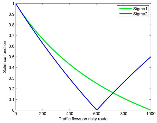
Figure 1. Schematic diagram of the relationship between ${\sigma }_1$ and ${\sigma }_2$.

Proposition 2.

When$n_R\in (0,n_{R_{split}})$, ${\sigma }_1>{\sigma }_2$—i.e., the good state is salient; when$n_R\in (n_{R_{split}},N]$, ${\sigma }_1<{\sigma }_2$—i.e., the bad state is salient; when$n_R=0$ and $n_R=n_{R_{split}}$, ${\sigma }_1={\sigma }_2$—i.e., no state is salient, where $n_{R_{split}}=\frac{2N{a}_2^2-2a_{2}c-a_{1}c+{\mathsf{\Gamma }}^{\frac{1}{2}}}{2a_2^2}$, with $\mathsf{\Gamma }$ being $c(a_1^{2}c+4a_2^{2}c+4a_1{a}_{2}c-4N{a}_1{a}_2^2)$.

Proof. 

We proceed the proof in three steps, which are the examination of monotonicity, the examination of salience ranking for special points, and the examination of salience equivalence.

(1)

Examination of monotonicity

As we see from the above discussions, both ${\sigma }_1$ and ${\sigma }_2$ are functions of $n_R$. First, we examine the monotonicity of ${\sigma }_1$ and ${\sigma }_2$ on $n_R$.

$$\frac{d{\sigma }_1}{d{n}_R}=\frac{-a_2(2c-a_2(N-n_R))-a_2(a_2(N-n_R))}{{(2c-a_2(N-n_R))}^2}=-\frac{2a_{2}c}{{(u^{-}(n_R)+u^{NR}(n_R))}^2}.$$

(23)

Because $a_2>0$ and $c>0$, as shown in Equation (17), $\frac{d{\sigma }_1}{d{n}_R}<0$ can be obtained—i.e., ${\sigma }_1$ is strictly decreasing as $n_R$ increases in the interval $\left[0,N\right]$.

When $0\le n_R\le n_{R_0}$, we obtain:

$$\begin{array}{ll}\frac{d{\sigma }_2}{d{n}_R}& =\frac{-(a_1+a_2)(2c-a_1{n}_R-a_2(N-n_R))-(a_2-a_1)(a_2(N-n_R)-a_1{n}_R)}{{(2c-a_1{n}_R-a_2(N-n_R))}^2}\hfill \\ & =-\frac{2a_1(c-a_2(N-n_R))+2a_2(c-a_1{n}_R)}{{(2c-a_1{n}_R-a_2(N-n_R))}^2}\hfill \\ & =-\frac{2a_1{u}^{NR}(n_R)+2a_2{u}^{+}(n_R)}{{(u^{+}(n_R)+u^{NR}(n_R))}^2}.\hfill \end{array}$$

(24)

Because all the utility functions are non-negative, as shown in Assumption 1, and $a_1>0$ and $a_2>0$, as shown in Equation (17), $\frac{d{\sigma }_2}{d{n}_R}<0$ can be obtained—i.e., ${\sigma }_2$ is strictly decreasing as $n_R$ increases in the interval $[0,n_{R_0}]$. By similar derivation, we obtain that ${\sigma }_2$ is strictly increasing as $n_R$ increases in the interval $(n_{R0},N]$.

(2)

Examination of salience ranking for special points

Next, we examine the salience relationship between ${\sigma }_1$ and ${\sigma }_2$ at several special points.

• When $n_R=0$, we have that $u^{+}(n_R)=c$, $u^{-}(n_R)=c$, and $u^{NR}(n_R)=c-a_{2}N$. Furthermore, ${\sigma }_1=\sigma (c,c-a_{2}N)$ and ${\sigma }_2=\sigma (c,c-a_{2}N)$. By ordering the property, we obtain ${\sigma }_1={\sigma }_2$.
• When $n_R=n_{R_0}$, we have ${\sigma }_1=\sigma (u^{+}(n_{R_0}),u^{NR}(n_{R_0}))$, and ${\sigma }_2=\sigma (u^{-}(n_{R_0}),u^{NR}(n_{R_0}))$. By ordering the property, we obtain ${\sigma }_1>{\sigma }_2$.
• When $n_R=N$, we have $u^{+}(n_R)=c$, $u^{-}(n_R)=c-a_{1}N$, and $u^{NR}(n_R)=c$. Furthermore, ${\sigma }_1=\sigma (c,c)$ and ${\sigma }_2=\sigma (c-a_{1}N,c)$. By ordering the property, we obtain ${\sigma }_2>{\sigma }_1$.

The combination of the examination of monotonicity and the examination of salience ranking for special points indicates that (1) there must be at least one point in the interval $[0,n_{R_0})$ that makes the salience equivalent between ${\sigma }_1$ and ${\sigma }_2$, and (2) there must be one point in the interval $(n_{R_0},N)$ that makes the salience equivalent between ${\sigma }_1$ and ${\sigma }_2$. Next, we examine the salience equivalence in these two intervals.

(3)

Examination of salience equivalence:

• Considering the interval $[0,n_{R_0})$, let ${\sigma }_1={\sigma }_2$, and we obtain:

  $$\frac{a_2(N-n_R)}{2c-a_2(N-n_R)}=\frac{a_2(N-n_R)-a_1{n}_R}{2c-a_2(N-n_R)-a_1{n}_R}.$$

  (25)

Solving Equation (25), we have $n_{R_1}=0$ and $n_{R_2}=-\frac{c-a_{2}N}{a_2}$. Because $c-a_{2}N\ge 0$, $n_{R_2}\le 0$. Therefore, if $n_{R_2}<0$, $n_{R_2}$ is not within the considered interval, it does not meet the requirement. Therefore, $n_R=0$ is the only solution that makes ${\sigma }_1$ equal to ${\sigma }_2$ in the considered interval.

2.

Considering the interval $(n_{R_0},N)$, let ${\sigma }_1={\sigma }_2$, and we obtain:

$$\frac{a_2(N-n_R)}{2c-a_2(N-n_R)}=\frac{a_1{n}_R-a_2(N-n_R)-a_1{n}_R}{2c-a_2(N-n_R)-a_1{n}_R}.$$

(26)

Solving Equation (26), we obtain $n_{R_3}=\frac{2N{a}_2^2-2a_{2}c-a_{1}c-{\mathsf{\Gamma }}^{\frac{1}{2}}}{2a_2^2}$ and $n_{R_4}=\frac{2N{a}_2^2-2a_{2}c-a_{1}c+{\mathsf{\Gamma }}^{\frac{1}{2}}}{2a_2^2}$ (i.e., $n_{R_{split}}$), where $\mathsf{\Gamma }=c(a_1^{2}c+4a_2^{2}c+4a_1{a}_{2}c-4N{a}_1{a}_2^2)$.

$n_{R_3}$ can be rewritten as $n_{R_3}=\frac{-a_{1}c-2a_2(c-a_{2}N)-{\mathsf{\Gamma }}^{\frac{1}{2}}}{2a_2^2}$, and combining that $c>0$, $c-a_{2}N\ge 0$, we obtain $n_{R_3}<0$. Therefore, $n_{R_3}$ is not within the feasible domain $(n_{R_0},N)$—i.e., it does not meet the requirements. That is, $n_{R_4}$ is the only solution that makes ${\sigma }_1$ equal to ${\sigma }_2$ in the considered interval.

Combining all the results and renaming $n_{R_4}$ as $n_{split}$, we complete the proof. □

According to Proposition 2, the relationship between ${\sigma }_1$ and ${\sigma }_2$ can be schematically shown in Figure 1. Here, we take $N=1000$ as an example. $a_1=0.2$, $a_2=0.3$, and $c=300$. Therefore,$n_{R_0}=600$. In particular, ${\sigma }_1$ is a convex function by verifying that $\frac{d^2{\sigma }_1}{d^2{n}_R}=4a_2^{2}c{[2c-a_2(N-n_R)]}^{-3}>0$; ${\sigma }_2$ is a convex function in the interval $[0,n_{R_0}]$ by verifying $\frac{d^2{\sigma }_2}{d^2{n}_R}=4[a_1(c-a_{2}N)+a_{2}c]{[2c-a_1{n}_R-a_2(N-n_R)]}^{-3}(a_2-a_1)>0$, and is a concave function on the interval $(n_{R_0},N]$ by symmetry.

Remark 1.

From Proposition 2, we see that, given the total travel demand and travelers’ utility functions, the salience ranking is fixed, which is irrelevant to the objective probabilities and travelers’ salience bias.

3.3.2. Equilibrium Analysis

According to Definition 3, the salient travel utility for the risky route with discrete ranking in a two-state world is written as

$$U_R(n_R)=\frac{p{\delta }^{k_p}{u}^{-}(n_R)+(1-p){\delta }^{k_{1-p}}{u}^{+}(n_R)}{p{\delta }^{k_p}+(1-p){\delta }^{k_{1-p}}},\forall n_R,$$

(27)

and the salient travel utility for the non-risky route is written as $U_{NR}(n_R)=u^{NR}(n_R),\forall n_R$ due to the normalization.

Before we start the formal analysis of the salient user equilibrium in the discrete case, we present the following results based on Proposition 1.

The salient travelers prefer the risky route $R$ to the non-risky route $NR$ if and only if:

$${\displaystyle \sum _{s\in S}{\delta }^{k_s}}{\pi }_s\left[u_s^R(n_R)-u_s^{NR}(n_R)\right]>0.$$

(28)

Here, $S=\{good,bad\}$. Therefore, at the salient user equilibrium, we have the equation:

$${\displaystyle \sum _{s\in S}{\delta }^{k_s}}{\pi }_s\left[u_s^R(n_R)-u_s^{NR}(n_R)\right]=0.$$

(29)

Motivated by Equation (29), we propose the following flow-dependent route preference function.

Definition 4.

The flow-dependent route preference function is formulated as:

$$V_{R\to NR}(n_R)=\{\begin{array}{cc}{V}_{1eq2}(n_R),\hfill & \mathrm{if}{n}_R=0;\hfill \\ V_{12}(n_R),\hfill & \mathrm{if}{n}_R\in (0,n_{R_{split}});\hfill \\ V_{1eq2}(n_R),\hfill & \mathrm{if}{n}_R=n_{R_{split}};\hfill \\ V_{21}(n_R),\hfill & \mathrm{if}{n}_R\in \left(n_{R_{split}},N\right]\hfill \end{array},$$

(30)

where$V_{12}(n_R)$corresponds to the situations in which${\sigma }_1>{\sigma }_2$—i.e., $n_R\in (0,n_{R_{split}})$; $V_{21}(n_R)$corresponds to the situations in which${\sigma }_2>{\sigma }_1$—i.e., $n_R\in (n_{R_{split}},N]$; $V_{1eq2}(n_R)$corresponds to the situations in which${\sigma }_1={\sigma }_2$—i.e., $n_R=0$and$n_R=n_{R_{split}}$.

Here, we have:

$$V_{12}(n_R)=\delta (1-p)\left[u^{+}(n_R)-u^{NR}(n_R)\right]+{\delta }^{2}p\left[u^{-}(n_R)-u^{NR}(n_R)\right],$$

(31)

$$V_{21}(n_R)=\delta p\left[u^{-}(n_R)-u^{NR}(n_R)\right]+{\delta }^2(1-p)\left[u^{+}(n_R)-u^{NR}(n_R)\right],$$

(32)

$$V_{1eq2}(n_R)=\delta p\left[u^{-}(n_R)-u^{NR}(n_R)\right]+\delta (1-p)\left[u^{+}(n_R)-u^{NR}(n_R)\right].$$

(33)

Based on the flow-dependence route preference function, we obtain that when $V_{R\to NR}>0$, the salient travelers prefer the risky route to the non-risky route; when $V_{R\to NR}<0$, the salient travelers prefer the non-risky route to the risky route; when $V_{R\to NR}=0$, a salient user equilibrium is obtained. Next, we present the formal results on the salient user equilibrium.

Proposition 3.

When$p\ne 1$, $n_R\in [0,n_{R_0}]$, there is no salient user equilibrium.

Proof. 

We proceed with the proof in two steps.

(1)

When $n_R=0$, we obtain $V_{R\to NR}=V_{1eq2}=\delta a_{2}N>0$—i.e., the salient travelers prefer the risky route to the non-risky route. Therefore, $n_R=0$ is not a salient user equilibrium.

(2)

Considering the interval $(0,n_{R_0}]$, we have $\frac{d{V}_{12}}{d{n}_R}=-(\delta (1-p)a_2+{\delta }^{2}p(a_1+a_2))<0$ when $p\ne 1$. Besides this,$V_{R\to NR}(n_{R_0})=V_{12}(n_{R_0})=\frac{\delta (1-p)a_1{a}_{2}N}{a_1+a_2}>0$. Therefore, we obtain $V_{12}(n_R)>0,\forall n_R\in (0,n_{R_0}]$—i.e., the salient travelers prefer the risky route to the non-risky route, and thus there is no salient user equilibrium in the considered interval. □

The intuitive explanation to Proposition 3 is that when $n_R\in [0,n_{R_0}]$, the travel utility of the risky route is larger than that of the non-risky route, no matter which state is salient. In this case, the salient travelers prefer the risky route.

Lemma 1.

Both$V_{12}(n_R)$and$V_{21}(n_R)$are strictly decreasing in the flow variable$n_R$. Moreover, at point$n_R=0$, $V_{1eq2}(0)>V_{12}^{-}(0)$; at point$n_R=n_{split}$, $V_{12}^{+}(n_{R_{split}})>V_{1eq2}(n_{R_{split}})>V_{21}^{-}(n_{R_{split}})$.

Proof. 

We have $\frac{d{V}_{12}}{d{n}_R}=-(\delta (1-p)a_2+{\delta }^{2}p(a_1+a_2))<0$ and $\frac{d{V}_{21}}{d{n}_R}=-({\delta }^2(1-p)a_2+\delta p(a_1+a_2))<0$ with all the parameters being positive, and thus both $V_{12}$ and $V_{21}$ are strictly decreasing in $n_R$ in their corresponding domains.

At point $n_R=0$, we have $V_{1eq2}(0)=\delta (1-p)a_{2}N+\delta p{a}_{2}N>0$ and $V_{12}^{-}(0)=\delta (1-p)a_{2}N+{\delta }^{2}p{a}_{2}N>0$. For a salient traveler, $\delta \in (0,1)$, and thus $V_{1eq2}(0)>V_{12}^{-}(0)$ by directly comparing $V_{1eq2}(0)$ with $V_{12}^{-}(0)$.

At point $n_R=n_{split}$, we have:

$$V_{12}^{+}(n_{R_{split}})=\delta (1-p)[a_2(N-n_{R_{split}})]+{\delta }^{2}p[a_2(N-n_{R_{split}})-a_1{n}_{R_{split}}]$$

$$V_{1eq2}(n_{R_{split}})=\delta (1-p)[a_2(N-n_{R4})]+\delta p[a_2(N-n_{R_{split}})-a_1{n}_{R_{split}}],$$

$$V_{21}^{-}(n_{R_{split}})={\delta }^2(1-p)[a_2(N-n_{R_{split}})]+\delta p[a_2(N-n_{R_{split}})-a_1{n}_{R_{split}}].$$

Because $n_{R_{split}}>n_{R_0}$, we have $a_2(N-n_{R_{split}})-a_1{n}_{R_{split}}<0$. For a salience traveler, $\delta \in (0,1)$, and thus $V_{12}^{+}(n_{R_{split}})>V_{1eq2}(n_{R_{split}})>V_{21}^{-}(n_{R_{split}})$ by directly comparing $V_{12}^{+}(n_{R_{split}})$ with $V_{1eq2}(n_{R_{split}})$, and comparing $V_{1eq2}(n_{R_{split}})$ and $V_{21}^{-}(n_{R_{split}})$. □

Here, − denotes the left limit, and + denotes the right limit. − and + also denote the bad state and good state, respectively. We assume this is clear from the context. The results of Lemma 1 are shown in Figure 2, Figure 3 and Figure 4. Proposition 3 shows that $V_{R\to NR}(n_R)>0$, $\forall n_R\in [0,n_{R_0}]$, and Lemma 1 shows the special value at $n_{R_{split}}$, which motivates the following logic for the analysis. For example, if $V_{R\to NR}(n_{R_{split}})<0$, combining that $V_{12}(n_R)$ is strictly decreasing within $(n_{R_0},n_{R_{split}})$, we can show that there exists a unique salient user equilibrium in this interval. All the following formal results are obtained based on the similar logic. Moreover, we find the common factor to shed light on the structure property, which is used for the sensitivity analysis in numerical experiments. This common factor is called discriminant, defined as $\eta =\frac{a_2(N-n_{R_{split}})}{a_1{n}_{R_{split}}-a_2(N-n_{R_{split}})}$, which is motivated by the discussions in Remark 1.

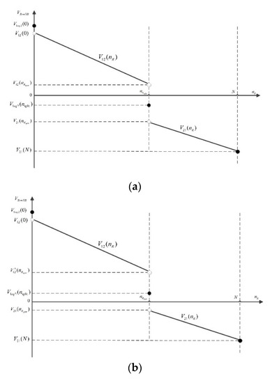
Figure 2. Schematic diagram of the proof in Proposition 4. (a) $\frac{\delta p}{1-p}\le \eta <\frac{p}{1-p}$; (b) $\frac{p}{1-p}<\eta \le \frac{p}{\delta (1-p)}$.

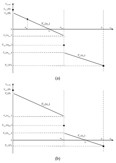
Figure 3. Schematic diagram of the proof in Proposition 5. (a) $\eta <\frac{\delta p}{1-p}$; (b) $\eta >\frac{p}{\delta (1-p)}$.

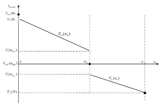
Figure 4. Schematic diagram of the proof in Proposition 6.

Proposition 4.

When$\frac{\delta p}{1-p}\le \eta <\frac{p}{1-p}$, or $\frac{p}{1-p}<\eta \le \frac{p}{\delta (1-p)}$, $n_{split}$is not a salient user equilibrium—i.e., there is no salient user equilibrium.

Proof. 

Substituting $\eta$ into $\frac{\delta p}{1-p}\le \eta <\frac{p}{1-p}$, we have:

$$\begin{array}{l}\frac{\delta p}{1-p}\le \frac{a_2(N-n_{R_{split}})}{a_1{n}_{R_{split}}-a_2(N-n_{R_{split}})}<\frac{p}{1-p}\\ \iff \{\begin{array}{c}\delta p(a_1{n}_{R_{split}}-a_2(N-n_{R_{split}}))\le (1-p)a_2(N-n_{R_{split}})\\ a_2(N-n_{R_{split}})(1-p)<p(a_1{n}_{R_{split}}-a_2(N-n_{R_{split}}))\end{array}\\ \iff \{\begin{array}{c}(1-p)\delta (c-(c-a_2(N-n_{R_{split}})))-{\delta }^{2}p(c-a_1{n}_{R_{split}}-(c-a_2(N-n_{R_{split}})))\le 0\\ (1-p)\delta (c-(c-a_2(N-n_{R_{split}})))-p\delta (c-a_1{n}_{R_{split}}-(c-a_2(N-n_{R_{split}})))>0\end{array}\\ \iff \{\begin{array}{c}(1-p)\delta (u^{+}(n_{R_{split}})-u^{NR}(n_{R_{split}}))-{\delta }^{2}p(u^{-}(n_{R_{split}})-u^{NR}(n_{R_{split}}))\le 0\\ (1-p)\delta (u^{+}(n_{R_{split}})-u^{NR}(n_{R_{split}}))-p\delta (u^{-}(n_{R_{split}})-u^{NR}(n_{R_{split}}))>0\end{array}.\end{array}$$

(34)

 □

That is, we obtain $V_{1eq2}(n_{R_{split}})<0\le V_{12}(n_{R_{split}})$ from the flow-dependent route preference function. When $\frac{p}{1-p}<\eta \le \frac{p}{\delta (1-p)}$, we obtain $V_{21}(n_{R_{split}})\le 0<V_{1eq2}(n_{R_{split}})$ from the flow-dependent route preference function following a similar procedure as before.

Therefore, in both cases, $\forall n_R\in [0,n_{R_{split}})$, $V_{R\to NR}>0$—i.e., the salient travelers prefer the risky route—and in $\forall n_R\in (n_{R_{split}},N]$, $V_{R\to NR}<0$, the salient travelers prefer the non-risky route. When $n_R=n_{split}$, $V_{R\to NR}<0$ for the first case, the salient travelers prefer the non-risky route, and $V_{R\to NR}>0$ for the second case, the salient travelers prefer the risky route. In summary, there is no salient user equilibrium for this situation.

Proposition 4 and its corresponding proof is schematically shown in Figure 2.

Proposition 5.

When$\eta <\frac{\delta p}{1-p}$or$\eta >\frac{p}{\delta (1-p)}$, there is a unique salient user equilibrium, and the final equilibrium traffic flows on risky route are$n_R^e=\frac{(1-p+\delta p)a_{2}N}{\delta p(a_1+a_2)+(1-p)a_2}$and$n_R^e=\frac{(\delta (1-p)+p)a_{2}N}{\delta p(a_1+a_2)+\delta (1-p)a_2}$, respectively.

Proof. 

When $\eta <\frac{\delta p}{1-p}$, we obtain $V_{12}(n_{R_{split}})<0<V_{12}(n_{R_0})$ as the aforementioned procedure. Solving $V_{12}(n_R)=0$, we obtain $n_R^e=\frac{(1-p+\delta p)a_{2}N}{\delta p(a_1+a_2)+(1-p)a_2}$. When $\eta >\frac{p}{\delta (1-p)}$, we obtain $V_{21}(N)<0<V_{21}(n_{R_{split}})$ as the aforementioned procedure. Solving $V_{21}(n_R)=0$, we obtain $n_R^e=\frac{(\delta (1-p)+p)a_{2}N}{\delta p(a_1+a_2)+\delta (1-p)a_2}$.

Therefore, in both cases we have $V_{R\to NR}>0,\forall n_R\in [0,n_R^e)$, where the salient travelers prefer the risky route, and we have $V_{R\to NR}<0,\forall n_R\in (n_R^e,N]$, where the salient travelers prefer the non-risky route. $V_{R\to NR}(n_R^e)=0$, $n_R^e\in (n_{R_0},n_{R_{split}})$ is an equilibrium solution. □

Proposition 5 and its corresponding proof are schematically shown in Figure 3.

Proposition 6.

When$\eta =\frac{p}{1-p}$, there is a unique salient user equilibrium, and the final equilibrium traffic flows on the risky route is$n_{split}$.

Proof. 

When $\eta =\frac{p}{1-p}$, we obtain $V_{1eq2}(n_{split})=0$ as the aforementioned procedure. Therefore, we have $V_{R\to NR}>0,\forall n_R\in [0,n_{split})$, where the salient travelers prefer the risky route, and we have $V_{R\to NR}<0,\forall n_R\in (n_{R_{split}},N]$, where the salient travelers prefer the non-risky route. $V_{R\to NR}(n_{split})=0$, $n_{split}$ is an equilibrium solution. □

Proposition 6 and its corresponding proof are schematically shown in Figure 4.

From the above propositions, we see that the interval $(0,\infty )$ is divided into five parts—i.e., $0<\eta <\frac{\delta p}{1-p}$, $\frac{\delta p}{1-p}\le \eta <\frac{p}{1-p}$, $\eta =\frac{p}{1-p}$, $\frac{p}{1-p}<\eta \le \frac{p}{\delta (1-p)}$, and $\eta >\frac{p}{\delta (1-p)}$. Each part corresponds to a different sufficient condition for the existence (or non-existence) of the salient user equilibrium. Next, we present our formal results about the travelers’ risk attitudes in a risky route choice based on the equilibrium results.

Proposition 7.

When$\eta =\frac{p}{1-p}$, no state is salient, and the travelers are risk-neutral; when$\eta <\frac{\delta p}{1-p}$, the good state is salient, and the travelers are risk-seeking; when$\eta >\frac{p}{\delta (1-p)}$, the bad state is salient, and the travelers are risk-averse.

Proof. 

When $\eta =\frac{p}{1-p}$, no state is salient; combing the results in Proposition 6, we obtain that Equation (33) becomes $\delta p[u^{-}(n_R)-u^{NR}(n_R)]+\delta (1-p)[u^{+}(n_R)-u^{NR}(n_R)]=0$. Rearranging this, we obtain the results with the expected utility theory—i.e., Equation (19), which indicates that travelers are risk-neutral.

When the good state is salient, its distorted probability will become larger, and thus the right-hand-side value of Equation (19) will become larger. Therefore, more travelers will choose the risky route—i.e., they are risk-seeking. Similarly, when the bad state is salient, its distorted probability will become larger, and thus the right-hand-side value of Equation (19) will become smaller. Therefore, more travelers will choose the non-risky route—i.e., they are risk-averse. □

4. More Discussions on the Salient User Equilibrium

In this section, we give more discussions on the salient user equilibrium.

4.1. Diminishing Sensitivity

From the above discussions, we see that the equilibrium analysis only concerns ordering and symmetry properties. Diminishing sensitivity is irrelevant. In this section, we examine the effect of diminishing sensitivity on the equilibrium analysis.

Here, we increase the intrinsic value $c$, denoted as $c^{\prime }$. We can also decrease the value of $c$ to illustrate the diminishing sensitivity, and similar discussions can be made accordingly. From Equation (21), we see that the value of $n_{R_0}$ remains the same, while the values of ${\sigma }_1$ and ${\sigma }_2$ are changed. In particular, we calculate the new splitting point as:

$$n_{{R^{\prime }}_{split}^{}}=\frac{2N{a}_2^2-2a_2{c}^{\prime }-a_1{c}^{\prime }+{\mathsf{\Gamma }}^{\frac{1}{2}}}{2a_2^2},$$

(35)

where $\mathsf{\Gamma }=c^{\prime }(a_1^2{c}^{\prime }+4a_2^2{c}^{\prime }+4a_1{a}_2{c}^{\prime }-4N{a}_1{a}_2^2)$.

Furthermore, when $n_R\in (0,n_{R_{split}^{\prime }})$, ${\sigma }_1>{\sigma }_2$; when $n_R\in (n_{R_{split}^{\prime }},N]$, ${\sigma }_1<{\sigma }_2$; and when $n_R=0$ and $n_R=n_{R_{split}}$, ${\sigma }_1={\sigma }_2$. Here, we continue to use the parameters shown in Figure 1, and only change the value of $c$ from 300 to 350 to show the effect of diminishing sensitivity, as presented in Figure 5.

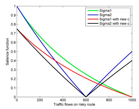
Figure 5. Schematic diagram of diminishing sensitivity.

From Figure 5, we see that the values of ${\sigma }_1$ and ${\sigma }_2$ decrease with the increase in the intrinsic value, which can be verified with the property diminishing sensitivity. Next, we discuss the impact of the increase in intrinsic value on the final salient user equilibrium. The value of the discriminant is changed due to the new splitting point. The above propositions show that if the original sufficient conditions are still satisfied with this new discriminant, the final equilibrium solution will remain the same. Otherwise, it will be different.

4.2. Relationship between $a_1$ and $a_2$

From the process of equilibrium analysis, we see that the relationship between $a_1$ and $a_2$—i.e., $a_1>(=,<)a_2$—has no impact on the equilibrium existence and uniqueness. However, the final salient user equilibrium can indeed be changed if we change the value of $a_1$ and $a_2$. Moreover, Proposition 3 is always true no matter what relationship is.

We show two representative situations for the utility functions in Figure 6. In Figure 6a, $\frac{a_1}{a_2}$ is large (e.g.,$\frac{a_1}{a_2}=10$), and the final equilibrium on the risky route could be large or small, which depends on the salient state. However, in Figure 6b, $\frac{a_1}{a_2}$ is small (e.g.,$\frac{a_1}{a_2}=0.2$), and the final equilibrium on the risky route is large. The explanation for this is the same as that for Proposition 3.

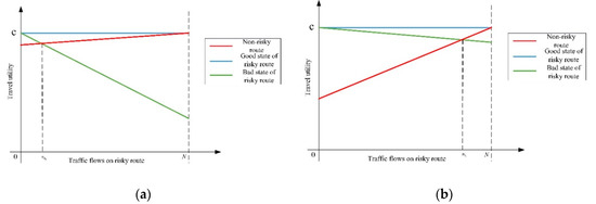
Figure 6. Two representative situations for the utility functions. (a) $\frac{a_1}{a_2}$ is large; (b) $\frac{a_1}{a_2}$ is small.

5. Numerical Experiments

In this section, we conduct the numerical experiments to demonstrate our theoretical findings. All the flow-dependent route preference functions are solved with the solve function in Matlab R2014a.

We consider $N=10000$ drivers traveling from the common origin to the common destination. Each traveler has to choose between a non-risky route and a risky route, and there are no other alternatives, as aforementioned.

The travel time utility functions for the non-risky route, the risky route in a bad state, and the risky route in a good state are $u^{NR}(n_R)=350-0.02(N-n_R)$, $u^{-}(n_R)=350-0.03n_R$, and $u^{+}(n_R)=350$, respectively. That is, $c=350$, $a_1=0.03$, and $a_2=0.02$. According to the aforementioned equations, $n_{R_0}=4000$ and $n_{R_{split}}=5363$. Given these parameters, the flow-dependent route preference function is written as:

$$V_{R\to NR}(n_R)=\{\begin{array}{l}\delta (1-p)(200-0.02n_R)+\delta p(200-0.05n_R),\mathrm{when}{n}_R=0,\\ \delta (1-p)(200-0.02n_R)+{\delta }^{2}p(200-0.05n_R),\mathrm{when}{n}_R\in (0,5363),\\ \delta (1-p)(200-0.02n_R)+\delta p(200-0.05n_R),\mathrm{when}{n}_R=5363,\\ {\delta }^2(1-p)(200-0.02n_R)+\delta p(200-0.05n_R),\mathrm{when}{n}_R\in \left(5363,10000\right].\end{array}$$

(36)

First, we consider two special cases for the salient travelers to demonstrate the propositions.

(1) Let $p=0.8$ and $\delta =0.5$; thus, $\frac{\delta p}{1-p}=2$, $\frac{p}{1-p}=4$, and $\frac{p}{\delta (1-p)}=8$. The value of the discriminant is $\eta =\frac{a_2(N-n_{R_{split}})}{a_1{n}_{R_{split}}-a_2(N-n_{R_{split}})}=1.3605$. Therefore,$\frac{a_2(N-n_{R_{split}})}{a_1{n}_{R_{split}}-a_2(N-n_{R_{split}})}<\frac{\delta p}{1-p}$. According to Proposition 5, we know that there is a unique equilibrium solution $n_R^e\in (4000,5363)$. Solving $V_{12}(n_R)=0.1\times (200-0.02n_R)+0.2\times (200-0.05n_R)=0$, we obtain $n_R^e=5000$.

Next, we set $p=0.8$, and change the value of $\delta$ from 0.34 to 0.99 (the range of $\delta$ is to ensure the existence of the salient user equilibrium). The salient equilibrium flow and the expected flow of Equation (19) on the risky route are shown in Figure 7. We see that the salient equilibrium flow is larger than the expected flow—i.e., the travelers are risk-seeking—when the good state is salient, which demonstrates Proposition 7. Furthermore, we see that the smaller the value of $\delta$ is—i.e., the larger the extent of the salience bias is—the larger the salient equilibrium flow is, and vice versa. That is, travelers’ risk-seeking extent depends the extent of salience bias.

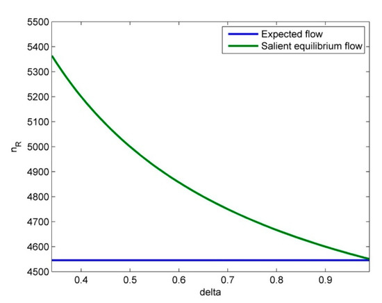
Figure 7. Salient equilibrium flow vs. the expected flow on the risky route with discrete ranking.

Here, we see that the probability for the risky route to have a small travel utility (i.e., in bad state) is high, but the travelers are risk-seeking, which sounds non-intuitive. The reason for this is that the salient travelers focus on the unusual aspect. When the risky route is in a bad state with a high probability, combining the above-mentioned travel utility functions and the equilibrium flows on the risky route shown in Figure 7, we obtain the utility difference in good state is larger—i.e., the good state is salient. Therefore, travelers are risk-seeking.

(2) Let $p=0.3$ and $\delta =0.8$; thus, $\frac{\delta p}{1-p}=0.3429$, $\frac{p}{1-p}=0.4286$, and $\frac{p}{\delta (1-p)}=0.5377$. The value of the discriminant is $\eta =\frac{a_2(N-n_{R_{split}})}{a_1{n}_{R_{split}}-a_2(N-n_{R_{split}})}=1.3605$. Therefore,$\frac{a_2(N-n_{R_{split}})}{a_1{n}_{R_{split}}-a_2(N-n_{R_{split}})}>\frac{p}{\delta (1-p)}$. According to Proposition 5, we know that there is a unique equilibrium solution $n_R^e\in (5363,10000]$.

Solving $V_{21}(n_R)=0.448\times (200-0.02n_R)+0.24\times (200-0.05n_R)=0$, we obtain $n_R^e=6565$.

Next, we set $p=0.3$, and change the value of $\delta$ from 0.32 to 0.99 (the range of $\delta$ is to ensure the existence of the salient user equilibrium). The salient equilibrium flow and the expected flow on the risky route are shown in Figure 8. We see that the salient equilibrium flow is smaller than the expected flow—i.e., the travelers are risk-averse—when the bad state is salient, which further demonstrates Proposition 7. Furthermore, we see that the smaller the value of $\delta$ is—i.e., the larger the extent of salience bias is—the smaller the salient equilibrium flow is, and vice versa. That is, travelers’ risk-averse extent depends the extent of salience bias.

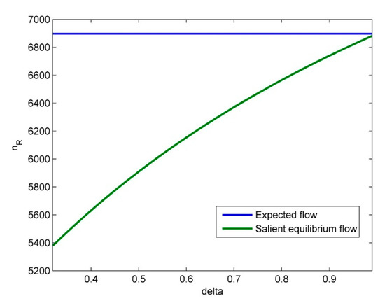
Figure 8. Salient equilibrium flow vs. the expected flow on the risky route with discrete ranking.

Here, we also see that the probability for the risky route to have a large travel utility (i.e., in good state) is high, but the travelers are risk-averse. This is also due to travelers’ salience characteristic. When the risky route is in a good state with a high probability, combining the above-mentioned travel utility functions and the equilibrium flows on the risky route shown in Figure 8, we obtain the utility difference in the bad state is larger—i.e., the bad state is salient. Therefore, the travelers are risk-averse.

Next, we show the change in the equilibrium traffic flow on the risky route with the change in $p$ and $\delta$ in Figure 9. Here, we increase the value of $p$ and $\delta$ from 0.01 to 0.99. The blue horn denotes the area in which there is no salient user equilibrium, and its corner denotes the special unique equilibrium when $\eta =\frac{p}{1-p}$ (travelers are risk-neutral). The warmer (cooler) color denotes the larger (smaller) value of the equilibrium flow on the risky route. The largest value is 9851, and the smallest value is 4024 in our test. The left part of Figure 9 corresponds to the situation where $\eta >\frac{p}{\delta (1-p)}$, and we see that (1) the larger $p$ is, the smaller the equilibrium traffic flow on the risky route is, and vice versa; (2) the larger $\delta$ is, the larger the equilibrium traffic flow on the risky route is, and vice versa. The right part of Figure 9 corresponds with the situation where $0<\eta <\frac{\delta p}{1-p}$, and we see that (1) the larger $p$ is, the smaller the equilibrium traffic flow on the risky route is, and vice versa; (2) the larger $\delta$ is, the smaller the equilibrium traffic flow on the risky route is, and vice versa. All the findings can be verified by the derivatives of $n_R^e$ with respect to $p$ and $\delta$ in each part, given the values of $a_1$, $a_2$, and $N$. If we change the value of parameters $a_1$, $a_2$, and $N$, the values will indeed be changed.

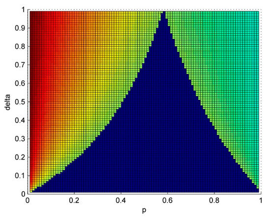
Figure 9. The impact of a change in $p$ and $\delta$ on the equilibrium traffic flow on the risky route.

6. Conclusions and Future Directions

This paper proposed a salient travel utility model to study travelers’ context-dependent route choice behavior on a risky traffic network. The psychological foundation of this new choice model is the proposed flow-dependent salience theory, which is an extension of the salience theory. Based on the salient travel utility model, we analyzed the long-run effect of this route choice model, and proposed the salient user equilibrium model. We followed the convention used in [35] to propose the salient travel utility model with a discrete ranking, and proposed an analysis procedure (the flow-dependent salience ranking analysis and flow-dependent route preference analysis) to study the user equilibrium. Finally, we theoretically proved the solution existence and uniqueness.

The equilibrium results show that travelers are not always risk-neutral, risk-seeking, or risk-averse, and this depends on the state that is salient. The main insights into travelers’ choice behavior are: (1) When no state is salient, travelers are risk-neutral; when a good state is salient, travelers are risk-seeking; and when a bad state is salient, travelers are risk-averse. (2) Travelers’ risk-neutral behavior is irrelative with the salience bias, while the extent of the risk-seeking or risk-averse behavior depends on the salience bias. A strong salience bias leads to a strong extent of travelers’ risk-seeking or risk-averse attitude. (3) When the travel utility on the risky route is small with a high probability (e.g., 0.7), the travelers are risk-seeking, and when the travel utility on the risky route is large with a high probability (e.g., 0.7), the travelers are risk-averse. (4) Risk-neutral is one special situation, where the solution to the flow-dependent route choice function and the solution to the salience ranking equivalence need to coincide. The main implication our findings can provide, for study and policy design considering travelers’ risk attitudes on the risky route choice, is that the salience characteristic can lead to non-intuitive risk attitudes for the travelers.

There are several limitations about the proposed methodology which merits further study. Firstly, although we propose a general framework for the salient travel utility in which multiple states of the world is considered, we only present the formal study on the two-state case in the equilibrium analysis. Secondly, we only focus on the two-route setting, and studying travelers’ salience characteristic in a general traffic network (three or more routes for each origin-destination pair) is important due to the practical use. This is a big open question (choice with three or more alternatives) even for the original salience theory [35]. Thirdly, we focus on the choice behavior only with one attribute, but many studies (e.g., [7,16]) show that travelers’ choice behavior might be affected by several attributes, such as travel time, travel time reliability, and travel cost. Fourthly, we assume that all the travelers know the objective probabilities, which can be relaxed based on travelers’ perceived probabilities. Fifthly, a behavioral experiment as conducted in [35] and [38] can be made to study travelers salient behavior empirically, which can provide some support to the parameter settings, and some parameter estimations can also be made accordingly. Finally, the new equilibrium model can shed light on some other problems—e.g., the congestion pricing and emission modeling. We plan to work on all these aspects in the future.

References

- Wardrop, J.G. Some theoretical aspects of road traffic research. Proc. Inst. Civ. Eng. 1952, 1, 325–362. [Google Scholar] [CrossRef]
- Beckmann, M.; McGuire, C.B.; Winsten, C.B. Studies in the Economics of Transportation; Yale University Press: New Haven, CT, USA, 1956. [Google Scholar]
- Gao, Z.; Wu, J.; Sun, H. Solution algorithm for the bi-level discrete network design problem. Transp. Res. Part B Methodol. 2005, 39, 479–495. [Google Scholar] [CrossRef]
- Wu, D.; Yin, Y.; Lawphongpanich, S.; Yang, H. Design of more equitable congestion pricing and tradable credit schemes for multimodal transportation networks. Transp. Res. Part B Methodol. 2012, 46, 1273–1287. [Google Scholar] [CrossRef]
- Sun, X.; Lu, H.P.; Chu, W.J. A low-carbon-based bilevel optimization model for public transit network. Math. Probl. Eng. 2013, 2013, 374826. [Google Scholar] [CrossRef]
- Umar, M.; Ji, X.; Kirikkaleli, D.; Xu, Q. COP21 Roadmap: Do innovation, financial development, and transportation infrastructure matter for environmental sustainability in China? J. Environ. Manag. 2020, 271, 111026. [Google Scholar] [CrossRef]
- Chen, A.; Zhou, Z. The α-reliable mean-excess traffic equilibrium model with stochastic travel times. Transp. Res. Part B Methodol. 2010, 44, 493–513. [Google Scholar] [CrossRef]
- Ji, X.; Ban, X.; Zhang, J.; Ran, B. Moment-based travel time reliability assessment with lasserre’s relaxation. Transp. B Transp. Dyn. 2019, 7, 401–422. [Google Scholar] [CrossRef]
- Knight, F.H. Risk, Uncertainty and Profit; Houghton Mifflin: Boston, MA, USA, 1921. [Google Scholar]
- Chen, Z.; Sim, M.; Xu, H. Distributionally robust optimization with infinitely constrained ambiguity sets. Oper. Res. 2019, 67, 1328–1344. [Google Scholar] [CrossRef]
- Mirchandani, P.; Soroush, H. Generalized traffic equilibrium with probabilistic travel times and perceptions. Transp. Sci. 1987, 21, 133–152. [Google Scholar] [CrossRef]
- Von Neumann, J.; Morgenstern, O.; Kuhn, H.W. Theory of Games and Economic Behavior (Commemorative Edition); Princeton University Press: Princeton, NJ, USA, 2007. [Google Scholar]
- Ban, X.J.; Ferris, M.C.; Tang, L.; Lu, S. Risk-neutral second best toll pricing. Transp. Res. Part B Methodol. 2013, 48, 67–87. [Google Scholar]
- Lo, H.K.; Luo, X.; Siu, B.W. Degradable transport network: Travel time budget of travelers with heterogeneous risk aversion. Transp. Res. Part B Methodol. 2006, 40, 792–806. [Google Scholar] [CrossRef]
- Watling, D. User equilibrium traffic network assignment with stochastic travel times and late arrival penalty. Eur. J. Oper. Res. 2006, 175, 1539–1556. [Google Scholar] [CrossRef]
- Ji, X.; Ban, X.J.; Li, M.; Zhang, J.; Ran, B. Non-expected route choice model under risk on stochastic traffic networks. Netw. Spat. Econ. 2017, 17, 777–807. [Google Scholar] [CrossRef]
- Ji, X.; Ban, X.; Zhang, J.; Ran, B. Subjective-utility travel time budget modeling in the stochastic traffic network assignment. J. Intell. Transp. Syst. 2017, 21, 439–451. [Google Scholar] [CrossRef]
- Kahneman, D.; Tversky, A. Prospect theory: An analysis of decision under risk. Econometrica 1979, 47, 263–292. [Google Scholar] [CrossRef]
- Tversky, A.; Kahneman, D. Advances in prospect theory: Cumulative representation of uncertainty. J. Risk Uncertain. 1992, 5, 297–323. [Google Scholar] [CrossRef]
- Bell, D.E. Regret in decision making under uncertainty. Oper. Res. 1982, 30, 961–981. [Google Scholar] [CrossRef]
- Xu, H.; Lou, Y.; Yin, Y.; Zhou, J. A prospect-based user equilibrium model with endogenous reference points and its application in congestion pricing. Transp. Res. Part B Methodol. 2011, 45, 311–328. [Google Scholar] [CrossRef]
- Zhang, C.; Liu, T.-L.; Huang, H.-J.; Chen, J. A cumulative prospect theory approach to commuters’ day-to-day route-choice modeling with friends’ travel information. Transp. Res. Part C Emerg. Technol. 2018, 86, 527–548. [Google Scholar] [CrossRef]
- Chorus, C.G.; Arentze, T.A.; Timmermans, H.J. A random regret-minimization model of travel choice. Transp. Res. Part B Methodol. 2008, 42, 1–18. [Google Scholar] [CrossRef]
- Daganzo, C.F.; Sheffi, Y. On stochastic models of traffic assignment. Transp. Sci. 1977, 11, 253–274. [Google Scholar] [CrossRef]
- Mahmassani, H.S.; Chang, G.-L. On boundedly rational user equilibrium in transportation systems. Transp. Sci. 1987, 21, 89–99. [Google Scholar] [CrossRef]
- Ahipasaoglu, S.D.; Meskarian, R.; Magnanti, T.L.; Natarajan, K. Beyond normality: A cross moment-stochastic user equilibrium model. Transp. Res. Part B Methodol. 2015, 81, 333–354. [Google Scholar] [CrossRef]
- Yan, C.-Y.; Hu, M.-B.; Jiang, R.; Long, J.; Chen, J.-Y.; Liu, H.-X. Stochastic ridesharing user equilibrium in transport networks. Netw. Spat. Econ. 2019, 19, 1007–1030. [Google Scholar] [CrossRef]
- Xiao, F.; Shen, M.; Xu, Z.; Li, R.; Yang, H.; Yin, Y. Day-to-day flow dynamics for stochastic user equilibrium and a general lyapunov function. Transp. Sci. 2019, 53, 683–694. [Google Scholar] [CrossRef]
- Di, X.; Liu, H.X.; Ban, X.J. Second best toll pricing within the framework of bounded rationality. Transp. Res. Part B Methodol. 2016, 83, 74–90. [Google Scholar] [CrossRef]
- Liu, J.; Zhou, X. Capacitated transit service network design with boundedly rational agents. Transp. Res. Part B Methodol. 2016, 93, 225–250. [Google Scholar] [CrossRef]
- Sun, L.; Karwan, M.H.; Kwon, C. Path-based approaches to robust network design problems considering boundedly rational network users. Transp. Res. Rec. 2019, 2673, 637–645. [Google Scholar] [CrossRef]
- Xu, H.; Yang, H.; Zhou, J.; Yin, Y. A route choice model with context-dependent value of time. Transp. Sci. 2017, 51, 536–548. [Google Scholar] [CrossRef]
- Finkelstein, A. E-ztax: Tax salience and tax rates. Q. J. Econ. 2009, 124, 969–1010. [Google Scholar] [CrossRef]
- Michel, A.; Zhao, J. Modeling saliency in transportation pricing: Optimal mixture of automobile management policies. In Proceedings of the Transportation Research Board 94th Annual Meeting, Washington, DC, USA, 11–15 January 2015. [Google Scholar]
- Bordalo, P.; Gennaioli, N.; Shleifer, A. Salience theory of choice under risk. Q. J. Econ. 2012, 127, 1243–1285. [Google Scholar] [CrossRef]
- Spitmaan, M.; Chu, E.; Soltani, A. Salience-driven value construction for adaptive choice under risk. J. Neurosci. 2019, 39, 5195–5209. [Google Scholar] [CrossRef] [PubMed]
- Nielsen, C.S.; Sebald, A.C.; Sørensen, P.N. Testing for Salience Effects in Choices under Risk. Available online: http://web.econ.ku.dk/sorensen/papers/TestingForSalienceEffects.pdf (accessed on 17 May 2020).
- Frydman, C.; Wang, B. The impact of salience on investor behavior: Evidence from a natural experiment. J. Financ. Forthcom. 2020, 75, 229–276. [Google Scholar] [CrossRef]
- Bordalo, P.; Gennaioli, N.; Shleifer, A. Salience theory of judicial decisions. J. Leg. Stud. 2015, 44, S7–S33. [Google Scholar] [CrossRef]
- Dertwinkel-Kalt, M.; Köster, M. Salient compromises in the newsvendor game. J. Econ. Behav. Organ. 2017, 141, 301–315. [Google Scholar] [CrossRef]
- Fochmann, M.; Wolf, N. Framing and salience effects in tax evasion decisions-an experiment on underreporting and overdeducting. J. Econ. Psychol. 2019, 72, 260–277. [Google Scholar] [CrossRef]
- Bordalo, P.; Gennaioli, N.; Shleifer, A. Salience and consumer choice. J. Political Econ. 2013, 121, 803–843. [Google Scholar] [CrossRef]
- Taylor, S.E.; Thompson, S.C. Stalking the elusive “vividness” effect. Psychol. Rev. 1982, 89, 155. [Google Scholar] [CrossRef]
- Kontek, K. A critical note on salience theory of choice under risk. Econ. Lett. 2016, 149, 168–171. [Google Scholar] [CrossRef]
- Connors, R.D.; Sumalee, A. A network equilibrium model with travellers’ perception of stochastic travel times. Transp. Res. Part B Methodol. 2009, 43, 614–624. [Google Scholar] [CrossRef]
- Wu, X.; Nie, Y.M. Modeling heterogeneous risk-taking behavior in route choice: A stochastic dominance approach. Transp. Res. Part A Policy Pract. 2011, 45, 896–915. [Google Scholar] [CrossRef]
© 2020 by the authors. Licensee MDPI, Basel, Switzerland. This article is an open access article distributed under the terms and conditions of the Creative Commons Attribution (CC BY) license (http://creativecommons.org/licenses/by/4.0/).