Article

Influence of Anthropogenic Noise for Predicting Cinereous Vulture Nest Distribution

by
Esther Ortiz-Urbina
1,
Luis Diaz-Balteiro
1,* and
Carlos Iglesias-Merchan
1,2
1
Department of Engineering and Forest and Environmental Management, Universidad Politécnica de Madrid, 28040 Madrid, Spain
2
CENERIC Research Centre, 28760 Tres Cantos, Spain
*
Author to whom correspondence should be addressed.
Sustainability 2020, 12(2), 503; https://doi.org/10.3390/su12020503
Submission received: 12 December 2019 / Revised: 6 January 2020 / Accepted: 7 January 2020 / Published: 9 January 2020

Abstract

:
Natural landscapes are increasingly under anthropogenic pressures, and concern about human impacts on wildlife populations is becoming particularly relevant in the case of natural areas affected by roads. The expansion of road networks is considered among the main factors threatening biodiversity due to their potential for disturbing natural ecosystems on large scales. Indeed, traffic noise pollution reduces the quantity and the quality of natural habitats, and umbrella species are frequently used as indicators of natural ecosystem health. In this sense, there is a variety of GIS-based ecological modeling tools that allow evaluation of the factors that influence species distributions in order to accurately predict habitat selection. In this study, we have combined the use of noise modeling tools and maximum entropy modeling (MaxEnt) to evaluate the relative importance of environmental variables for Cinereous vulture (Aegypius monachus) nesting habitat selection within a mountainous forest in Spain. As a result, we found that spatial negative influence of roads on wildlife due to road traffic disturbance may have been traditionally overestimated when it has been inferred from distance measurements of wildlife behavior in road surroundings instead of from considering road traffic noise level exposure. In addition, we found a potential risk threshold for cinereous vulture breeding around roads, which ties in with a Leq24h level of 40 dB(A). This may be a useful indicator for assessing the potential impact of human activities on an umbrella species such as, for instance, the cinereous vulture, whose breeding does not take place where road traffic Leq24h levels are higher than 40 dB(A).

1. Introduction

Natural landscapes are under continuous pressure and modifications from diverse human activities [1]. Due to the growing human encroachment within wildlife habitat, the impact of human activities on natural areas has received increased attention from researchers and ecologists during the last decades [2]. However, the effects of human disturbance on wildlife behavior, population dynamics and life history may still be poorly documented [3]. Indeed, animals are assumed to choose particular habitat attributes and food resources to maximize their fitness but they cannot always correctly assess habitat quality [4]. Thus, large spatial and temporal scale consequences of these trends remain unknown [5]. However, concern about human impacts on wildlife populations is increasingly relevant in case of high road densities. Mainly in protected areas and peri-urban environments, where roads often have regular traffic from tourists and local residents [6].
Road networks may contribute to the decrease in both the quantity and the quality of natural habitats, which is currently considered to be among the main factors threatening biodiversity [7,8]. Europe is particularly highly fragmented by transport infrastructure, which do not leave many natural areas unoccupied and constrain the effectiveness of conservation policies [9]. Half of the continent is within 1.5 km of a paved road or a railway line and almost a quarter of all Europe’s land area (22.4%) is located within 500 m of the nearest transport infrastructure [10]. The level of exposure to human infrastructure varies throughout the distribution of a species, and animals may shift their habitat selection to avoid disturbance by road networks within their home ranges. Wildlife that use habitats that are adjacent to roads experience disturbance due to traffic noise, which is considered a severe disruptor of the natural environment [5]. Nevertheless, traffic volume and distance from the road are the main variables considered for evaluating potential effects of transport infrastructure on wildlife communities. Indeed, several authors have quantified the reduction in the species richness and relative abundance as extending up to 1000–1200 m from road edges [11]. This distance from the edge of the road, over which significant ecological effects can be detected, is called the road-effect zone [12]. Following this approach, the habitat-loss impact is estimated as a buffer map that may range several hundred meters from road margins according to the road type and traffic volume [7].
Among the main negative effects of roads, traffic emissions such as noise are considered to be the cause of long-distance avoidance of roads [13]. Nevertheless, this component of road avoidance depends on traffic parameters such as traffic density, but not necessarily on the size of the road [14]. The intensity of the noise perceived in the surroundings of the roads fades with distance [15], although the noise level is not always reflected by the distance to roads. Depending on the landscape, there may be sections protected by obstacles (e.g., cutting slopes, constructions), or by the land itself (e.g., embankments, natural hollows) that, even being a few meters from the road edges, are not affected by any traffic disturbance [16]. Modern environmental noise modeling tools studies have allowed researchers to isolate noise from potentially confounding variables, and they have evidenced that noise alone can negatively affect wildlife [17,18]. In this sense, there are a variety of GIS-based modeling resources that provide a huge potential as prediction tools for providing quantitative and spatially explicit assessment of impacts on valued biodiversity components [19]. In particular, it is common practice to use species distribution modeling tools, which are becoming increasingly popular in conservation, especially in the case of threatened and endangered species [20]. Most of species show nonrandom habitat selection behavior because of environmental variables that may restrict habitat availability [21]. Therefore, it is of great importance for wildlife managers to consider factors that influence species distributions in order to accurately predict habitat selection [22].
Cinereous vulture (Aegypius monachus) is a scavenger species situated at the top of the food chain, and it is catalogued as ‘near threatened’ by the IUCN with a decreasing population outside Europe [23]. This is sensitive to disturbances caused by humans; it is considered to be an indicator of quality of natural ecosystems. Thus, cinereous vulture is considered an umbrella species [24,25]. Cinereous vultures nest on mature trees in woods on slopes far away from human presence [8,26,27] and from roads [24,28,29,30,31,32,33], since an important variable in the breeding success of this bird is the absence of any human disturbance [34]. Prior studies on the influence on nest site selection have assessed the effect of the roads in terms of the Euclidean distance to nest site locations [24,28,29,30,31,35,36]. Other authors report human influence as a function of the distance to an urban area [14] or of the density of the population in the Californian condor (Gymnogyps californianus) [37] or in the Griffon vulture (Gyps fulvus) [38]. However, road-effect zones could be more realistic and effectively mapped by using noise contour lines (a continuous line on a map that represents equal levels of noise exposure) instead of constant Euclidean distances [23].
Nevertheless, there is still a need of studies documenting the population-level effects of roads and traffic [5]. One way to explore this is facilitated by species distribution models, which are numerical techniques aimed at giving detailed predictions of distributions by relating them to the presence or abundance of one or several species with environmental information [39,40,41]. However, there is still a lack of deep knowledge of noise reference levels and behavioral responses of wildlife populations [19]. The main objective of this study is to appraise differences between considering road traffic noise and Euclidean distance to road margins when assessing the potential impact of road traffic disturbance on a nesting colony of cinereous vultures in central Spain. In order to assess the dimension of the road-effect zone, we considered building two scenarios (Scenario #1 and Scenario #2) to be computed in MaxEnt, one of the most common pieces of software for predicting species distribution [42,43]. In Scenario #1 we considered road traffic noise and seven of the most influential factors in the definition of the potential cinereous vulture nesting habitat according to literature within the study area. In Scenario #2 we repeated the same steps, but we used the traditional variable ‘distance to roads’ instead of road traffic noise.

2. Material and Methods
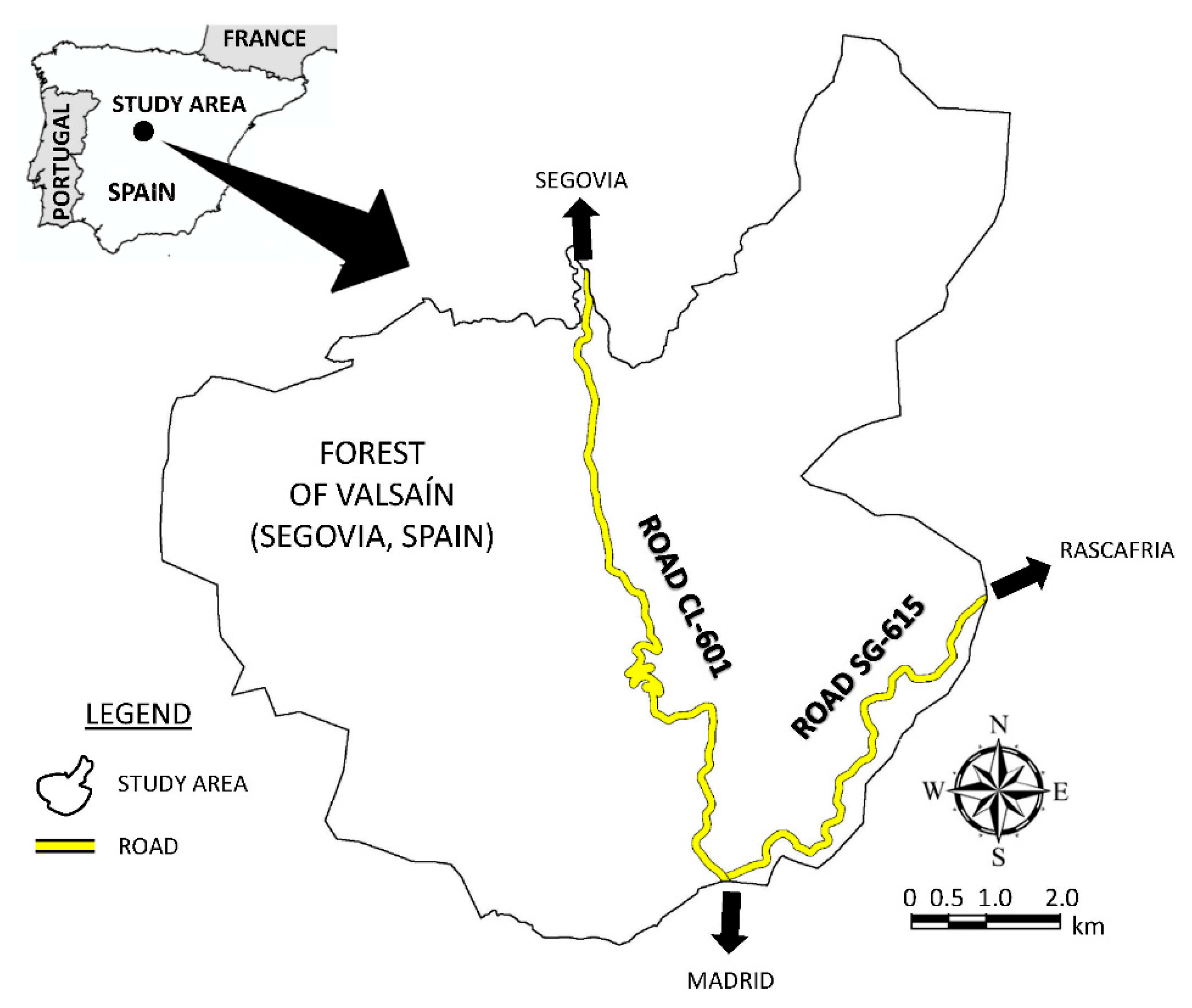
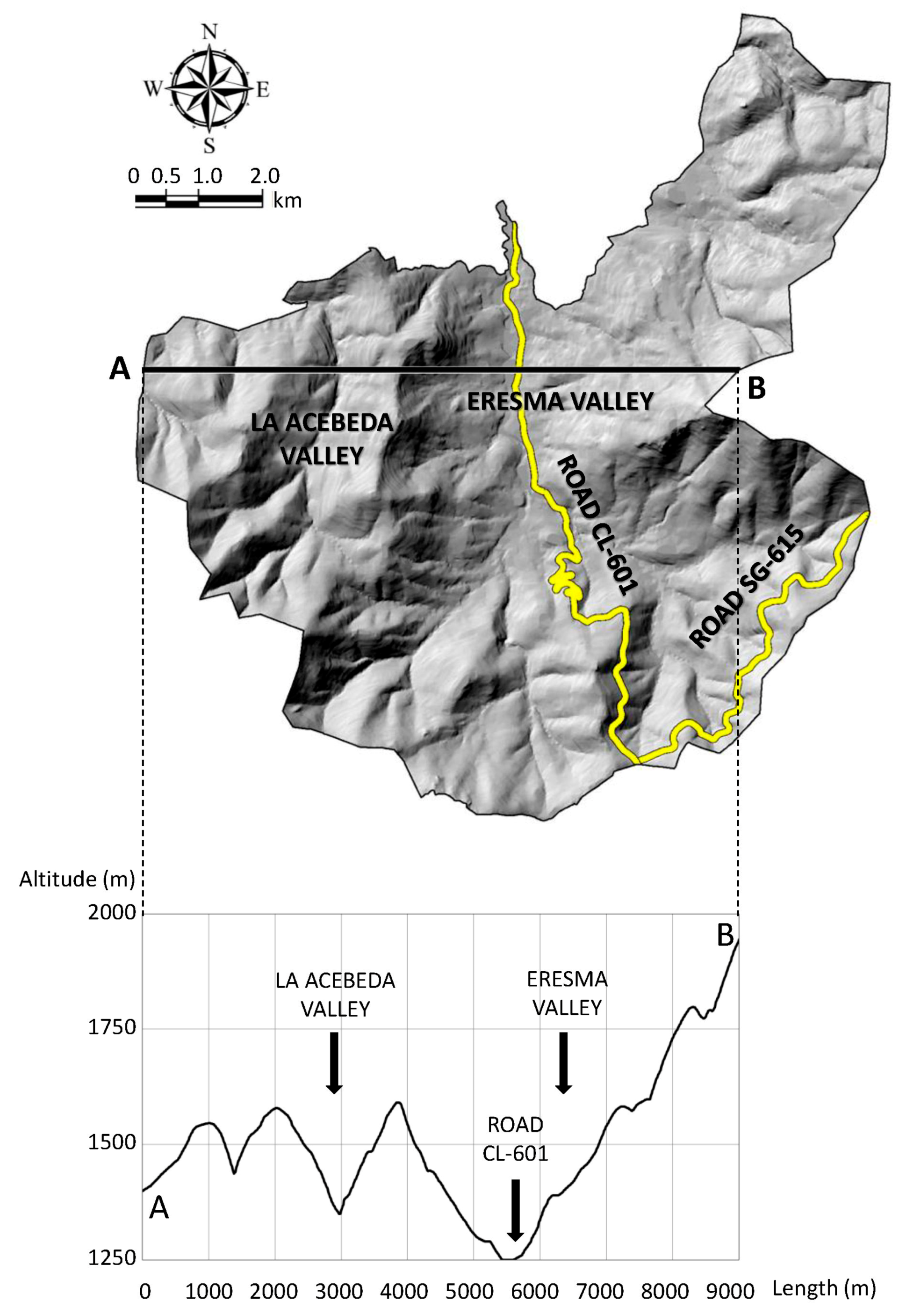
2.1. Study Area

The study area is located in the forest of Valsaín which extends over approximately 7600 hectares of surface on the north-facing slopes of the Sierra de Guadarrama (province of Segovia, in central Spain). The forest of Valsaín is an emblematic forest in Spanish forestry history and is under the jurisdiction of Sierra de Guadarrama National Park. The main tree species is Scots pine (Pinus sylvestris L.) and 131 nests of cinereous vulture have been inventoried [44,45]; it is worth mentioning that this species needs large areas of an appropriate habitat for its well-being [46]. The first forest management plan dates from 1889 but, in recent years, its management has become more multifunctional. Indeed, nowadays close attention is paid to aspects like biodiversity conservation. However, tourism has become one of the main economic sectors in the area with mass tourism becoming more visible in 2013, when the Sierra de Guadarrama was declared a national park [47]. The forest of Valsaín is just one hour by car from the city of Madrid (3,225,000 inhabitants) and only 20 min by car from the city of Segovia (150,000 inhabitants). The study area is crossed by road CL-601, which is the shortest route between Madrid and Segovia (Figure 1). In addition, the Southeastern limit of the forest of Valsaín is almost coincident with the trace of road SG-615 to the neighboring valley of Lozoya (Madrid).

2.2. Definition of Scenarios

The bibliography was reviewed in order to obtain the variables identifying the most influential factors in cinereous vulture nesting in the literature (Table 1). Noise level in nesting sites due to road traffic (Noise) and seven other variables were selected to define what we called Scenario #1: Noise, distance to trails (TrailD), terrain slope (Slope), average slope aspect (Aspect), land altitude (Altitude), tree density at stand level (TreeD), average tree height at stand level (TreeH) and distance to the nearest nest (NestD). Part of these data was obtained from the current forest management plan, and thematic maps with orography data (10 × 10 m resolution) were based on the official 1:25,000 scale topographic digital maps (10 m contour lines) from the Spanish National Geographic Institute (Instituto Geográfico Nacional). We adopted the equivalent continuous sound pressure level (Leq), in A-weighted decibels (dB(A)), characterizing a 24-h period (Leq24h) in a typical year as a reliable noise indicator [48].
Other temporal averaging alternatives could be used in case of assessing particular behavioral effects on wildlife (e.g., behavioral changes in singing species, breeding success). However, the use of Leq24h and the annual average daily traffic data (AADT) were considered the most appropriate in accordance with the aim of this case study (i.e., to assess a potential global influence of traffic noise pollution using a long-term average sound level index) and also to promote its potential applicability in a variety of fields (e.g., environmental impact assessment of transport infrastructure, public use management of natural protected areas). Indeed, the breading season may last from February until September or October. Moreover, we defined a second scenario called Scenario #2 composed by the same variables but by considering distance to roads (RoadD) instead of Noise, which is the variable more frequently used to assess the effects of road disturbance on cinereous vulture nesting habitat in the literature to date.
An analysis of correlation was carried out to find out the multi-collinearity between variables (Table 2). As data were not normally distributed (Kolmogorov–Smirnov test), the nonparametric Kendall’s tau-b (Τb) correlation coefficient was used, which is considered a nonparametric alternative to the Pearson’s correlation test when data fail one or more of the assumptions of this test. In the case of the correlation between the environmental variables being a high one (Table 2), the percent contribution of each variable to the potential species distribution model may be misleading [52]. In our case, it turned out to be recommendable to run the Jackknife test in MaxEnt to evaluate the relative importance of environmental variables for the cinereous vulture within the forest of Valsaín. This test makes alternative estimations of which variables are the most important ones in the model [51], and the model’s performance is evaluated according to its capacity to predict their localization excluding the set of data [20]. When user runs the Jackknife test, a number of models are created and a graph shows the gain of using each variable in isolation.

2.3. Noise Modeling

A road traffic noise map was calculated within the study area following the French national computation method referred to in the French standard “XPS 31-133”. We used the Computer Aided Noise Abatement software (CadnaA Version 2018 MR 1, 32-bit) to predict road traffic sound pressure levels (dB(A)) in road surroundings. Calculations were based on a digital elevation model which was built from the official 1:25,000 scale topographic digital maps. Road traffic speed and traffic density data were obtained from the Road and Transport Department of the Regional Government of Castile and León (Junta de Castilla y León). It is worth noting that AADT showed approximately 5000 vehicles per day on the road CL-601 and 650 vehicles on the road SG-615. The average speed on CL-601 was considered to be 65 km/h (55 km/h for heavy vehicles) and on SG-615, the average speed was considered to be 60 km/h (55 km/h for heavy vehicles).

2.4. Cinereous Vulture Potential Distribution Modeling

A variety of methodologies (e.g., MaxEnt, generalized linear models (GLM), genetic algorithm for rule-set production (GARP) modeling system (GMS)) can be used to find out the potential distribution of a certain species. We used the maximum entropy model (Maxent version 3.3.3; http://www.cs.princeton.edu/wschapire/maxent/) [52] in this study because it has shown itself to perform better with small sample sizes compared to other modeling methods [53]. To set up potential distribution models of cinereous vulture within the forest of Valsaín, in this case, presence data provided by Valsaín managers were used. The potential distribution describes the places with the most suitable conditions for the survival of this species [54]. MaxEnt permits the estimation of the potential distribution of the species using a list of locations with its presence, and a set of environmental variables [39,40,55], including small extension data [56], starting from incomplete information [52].
In our case study we have defined a convergence threshold of 10−5, a maximum of 5000 iterations, 20 replicates and a random test percentage of 25. Therefore, the program selects 25% of the random simple records to calculate the reliability of the prediction [57]. Thus we are able to validate the whole model instead of small sample sizes, which is a common problem in ecology when working with rare animal species such as raptors [58]. We thus obtained the potential distribution map of cinereous vultures within the study area in both Scenarios #1 and #2. In addition, we calculated: (i) The value of the area under the receiver operating curve (AUC), which is an index that supplies a single general precision measurement [59], and (ii) the percentage contribution of the environmental variables to the final result [51].

3. Results

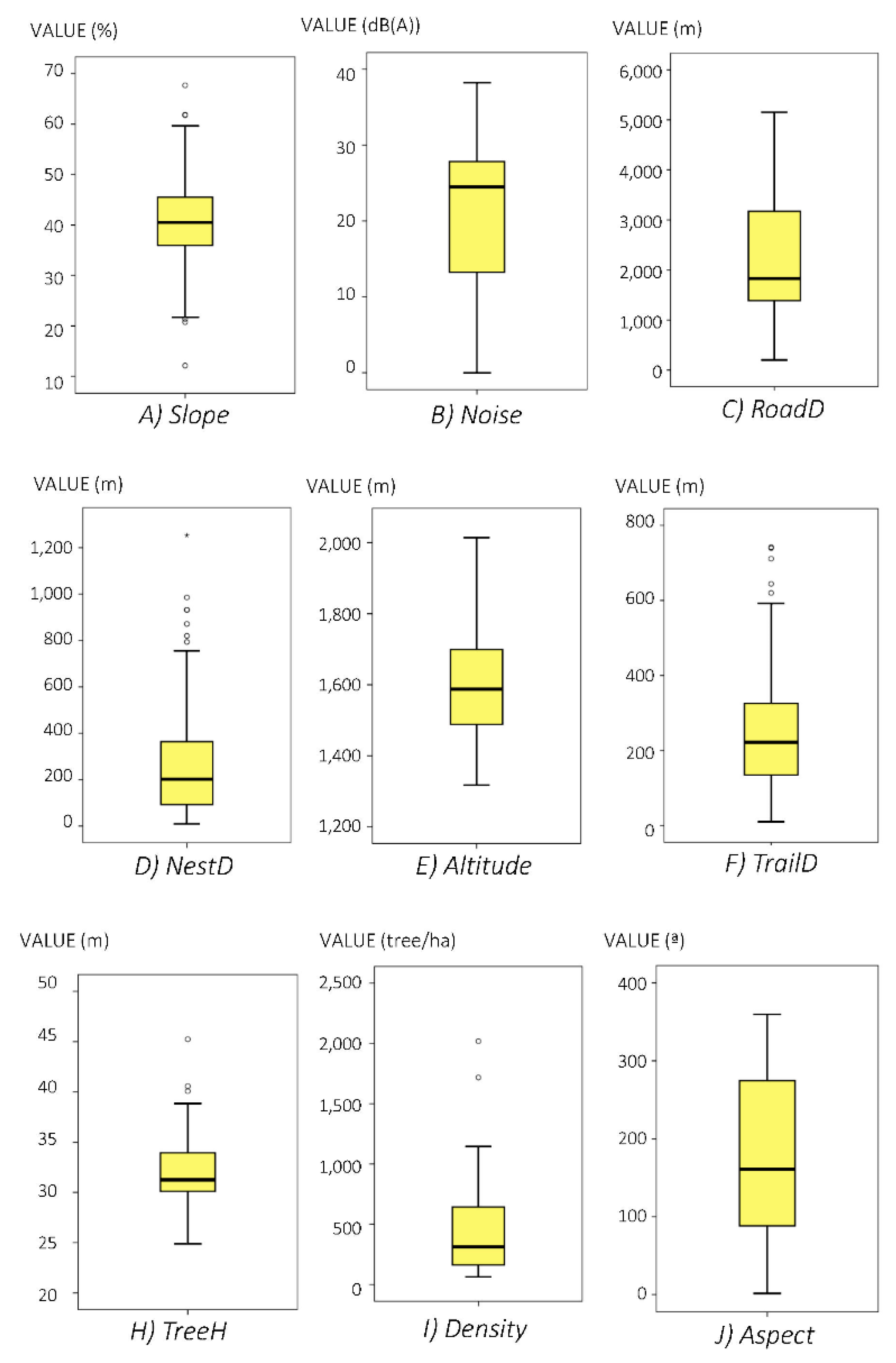
3.1. Descriptive Results

Cinereous vultures apparently locate their nests at an average distance of 2200 m from road margins (which ranged between 200 and 5000 m), and at an average distance of 250 m from unpaved trails. These latter distances oscillated from less than 10 m to up to 740 m (Figure 2). In relation to road traffic noise, it is worth noting that there were no nest site locations exposed to Leq24h levels higher than 39 dB(A). On the other hand, the distance to the nearest nest was between 10 and 1250 m. With regard to the orographic variables, nest sites were located on terrain slopes that ranged between 12 and 68% and at altitudes from approximately 1300 to 2000 m. With respect to the variables related to forest management, nest sites in the forest of Valsaín were located in stands with average tree densities of about 400 trees/ha and average tree heights of 30 m (ranging between 25 up to 45 m).

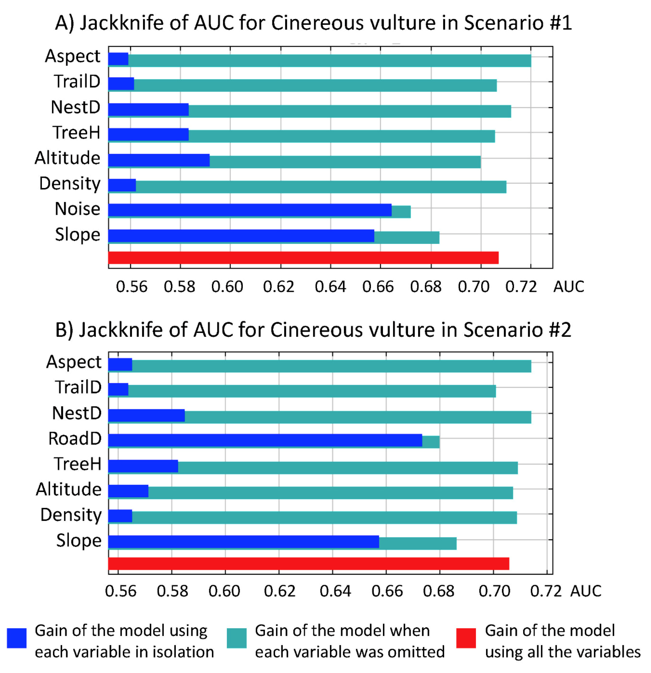
3.2. Applicability of the Model and Percent Contribution.

The predictive accuracy of the models (AUC values) scored higher than 0.70 in both Scenarios #1 and #2 (Table 3). Moreover, the first variable ranked according to its percent of contribution was the variable Slope in both Scenarios #1 and #2. However, in Scenario #2, the percent contribution of the variable RoadD (27.0%) was significantly higher (7.6 points) than the variable Noise (19.4%) in Scenario #1. In addition, it should be noted that the remaining six variables had a lower value of percent contribution in Scenario #1 than in Scenario #2. Higher differences were found in Altitude (4.1%) and TrailD (3.0%) and lower differences were found in TreeH (0.4%) and Aspect (0.3%), which were always higher in Scenario #1 than in Scenario #2.
The Jackknife test for evaluating the relative importance of environmental variables for cinereous vulture potential nesting habitat within the forest of Valsaín showed that road disturbance, whether it is expressed in terms of Noise (dB(A)) or RoadD (m), was the most important factor in both Scenarios #1 (Figure 3A) and #2 (Figure 3B). According to the Jackknife test, the second variable in importance was Slope. Therefore, in the absence of roads, Slope appeared to have the most useful information by itself. However, differences in the AUC value between the first variable (Noise in Scenario #1 or RoadD in Scenario #2) and Slope were higher in Scenario #2 in favor of RoadD.

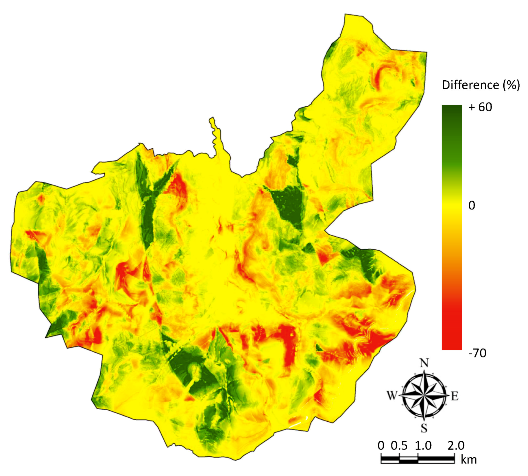
3.3. Potential Nesting Areas

MaxEnt modeling output maps give insight into the relative suitability of one place in relation to another place for cinereous vulture nesting location. Apparently, there did not seem to be any significant difference between the distribution probability categories (ranges of 10%) in Scenarios #1 and #2 (Table 4) when expressed in a percentage over the total surface of the study area. The prediction map revealed that a greater probability of occupancy than 0.8 was found in only 2.0% of the study area in Scenario #1 and 2.4% of the study area in Scenario #2. However, it represents a quantitative difference of 20% in the total surface of suitable places with high probability of occupancy (greater than 0.8) between both scenarios. In addition, spatial difference in the resulting maps when estimating the distribution probability of nesting sites within the study area in Scenarios #1 and #2 was more evident when it was mapped (Figure 4).

4. Discussion

First, it is of interest to mention that AUC values of >0.7 indicate a high measure of predictive accuracy [49] in our models. In addition, there are two major findings in this work. The first finding reveals that the influence of road-effect zone based on distance from nest site locations to road margins may be overestimated in previous research. The second major finding reveals the existence of an exclusion area for cinereous vulture breeding, in which road traffic Leq24h levels were over 40 dB(A).
According to our results, an overestimation of the role of roads may occur when we try to measure road disturbance effects on wildlife based on variables such as the distance from animals or their nesting sites to the road margins. For instance, roads seem to be the second variable in importance for cinereous vulture nesting within the study area (either assessed by Noise in Scenario #1 or by RoadD in Scenario #2). Nevertheless, the percent contribution of RoadD in Scenario #2 was significantly higher (7.6 points) than when we tried to measure the road-effect zone based on Noise level (19.4%) due to emissions from road traffic in Scenario #1. Furthermore, the Jackknife test for evaluating the relative importance of environmental variables may also contribute to misinterpreting the effect of road traffic in some studies, as occurred in our case. In fact, the Jackknife test maximized the role of RoadD in Scenario #2.
It has been accepted that the presence of a road may degrade ecosystems due to both biophysical alterations and road traffic noise [7]. We do not doubt the apparent importance of disturbances from roads for the cinereous vulture (or any other species’ breeding colonies) but we disagree with common quantification methods. Despite this, this species has several times been defined as being sensitive to disturbance [10,29,31,32,49,50,60]. According to our measurements, distance from the nearest nest site to the road margins was approximately 200 m, although the most frequent distances from roads range between 1000 and 2500 m. However, measuring road distances based on statistical techniques and geographic information system (GIS) tools may have important consequences, depending on a set of considerations. For instance, when the variable RoadD measured on the map is considered, any pixel in the study area has a value for this variable with a negative gradient from the road. However, when the road-effect zone due to traffic disturbance is quantified in this way, it is not taken into account that the road may be located at the other side of a hill, which completely shields the potential noise emissions (Figure 5). Thus it makes no sense to measure RoadD as such in the whole study context. A matter that can be addressed in a more realistic way by noise modeling [8].
Nests situated in La Acebeda Valley (Figure 5) are not affected by being nearer or further from the road that is in Eresma Valley. However, in considering RoadD as a continuous variable within the whole study area, a potential effect to the Eresma Valley road is attributed when predicting a suitable habitat for the cinereous vulture in La Acebeda Valley. Namely, in this case, an error is committed that is equivalent to making a map of heights of trees that present non-zero continuous values in places where there are no trees. This is a limitation to be considered in habitat modeling because it may lead to an exaggerated distortion in the prediction of habitat suitability because of the extrapolation of environmental data outside its geographic area of influence [61,62,63,64]. Criticism in the conventional modeling of habitat prediction is that most users collect, not the most appropriate environmental variables, but rather those that are easily feasible in digital formats across broad geographic extents (e.g., RoadD) [65]. In fact, indirect variables (i.e., those not having direct effects on the physiology of the species), such as RoadD in La Acebeda Valley, should be avoided, because the correlation between indirect variables and more direct ones may be location-specific and need not be linear [61]. Thus, we should control the broad-scale of geographic data and the inclusion of uninformative data for an ecological model [63]. This could be considered by modeling the type of real disturbance that it is meant to be assessed. For instance, a variety of factors affecting noise exposure predictions need to be contemplated in the case of assessing effects or effect zones on the wider ecosystem for which the modeling of sound propagation has been established as a useful discipline during recent years [66,67,68]. While sound pressure level at a receiver decreases with the distance from the noise source, it is not the only factor influencing the propagation of sound (e.g., type of pavement, trace of road sections, vehicle density, average speed, percentage of heavy vehicles, terrain slope, vegetation coverage, ground absorption, meteorological conditions).
Regarding TrailD, this variable turned out to be irrelevant, which may be linked to the fact that it appears that many raptors can tolerate a low intensity and short duration of human disturbance near their nests [58]. However, the cinereous vulture is commonly considered to be sensitive to disturbance, making vultures avoid areas of intensive activity, but this argument is mostly inferred from measuring the distance to nest sites distributed around roads and villages [24,28,29,31,32,49,50,60]. In general, tree-nesting big raptors are known to nest at a greater distance from roads, where it is assumed that disturbance levels become weaker [36]. Therefore, raptors have often been considered to be indicators of ecosystem health or umbrella species [24]. In this sense, habitat suitability models can provide the statistical framework linking environmental variables to the occurrence locations, which makes this result of importance for conservation management. However, in some cases, results should be interpreted with caution and require careful consideration as they can produce misleading comparative results [62,65].
In relation to the geomorphologic model, nest sites were mostly situated on steep slopes and at high altitudes. Slope is the variable that presented the highest percent contribution for the target species in both Scenarios #1 and #2. On the contrary, exposure did not turn out to be an important factor. Slopes, together with tree selection, are supposed to provide protection against predation (which is extremely rare in this case) or disturbances since the latter are less likely to occur in rugged areas, and selected trees are supposed to provide good views for detecting aerial predators at a distance [26,33,60]. This main result agrees with previous studies conducted in Spain and Greece, which showed common nesting habitat patterns for cinereous vultures, where nests were located on steep slopes [24,29,31,32,49,60]. In particular, Morán-López et al. [28,50] have gone so far as to define these areas with steep slopes far from human disturbance as being the preferred breeding sites for cinereous vultures. In addition to the above, another probable reason to explain the use of slopes may be the need for the exposure of nests to climate factors. Moreover, Donázar et al. [24] noted that the existence of slope winds may enhance flight energy during foraging. This preference seems to be a key distinguishing factor compared to other forest raptors, on which several studies reported that relatively few species select steep slopes for nesting purposes [58].
Regarding forest variables, several authors have found that nests of cinereous vultures are typically built in large trees in larger homogenous patches within forested mountainous areas [31,69], although tree species may vary depending on the region [49]. Poirazidis et al. [29] give TreeH and total number of trees as significant variables but Mihoub et al. [33] explained that cover density, as well as tree species, appears to be of secondary importance if the size and height of trees are large enough. According to our results, percentage contributions confirm the secondary role of these variables once the habitat is characterized and clearly dominated by pure even-aged Pinus sylvestris within the study area, while mixed Pinus sylvestris–Quercus pyrenaica stands are found in lower slopes at elevations of below 1400 m a.s.l. [45]. In spite of the fact that the dominant vegetation consists of typical Mediterranean trees such as holm oak (Quercus ilex) and cork oak (Q. suber), in other breeding areas of cinereous vulture in the Iberian Peninsula [31] the nesting habitats selected in the forest of Valsaín are clearly influenced by Slope in accordance with the above mentioned studies.
In our case study, distance to the nearest nest ranged between 10 and 1250 m (265 m on average), and the percentage contribution of NestD was the third variable in order of importance in both Scenarios #1 and #2. Moreover, Guerrero-Casado et al. [49] described a wide range of between 60 and 5350 m of distance to the nearest neighboring nest (1000 m on average) in a breeding colony of cinereous vultures in southern Spain. This variable has a relevant biological meaning and it is considered to be a key factor in the population dynamics that can influence stability and persistence in the long term [70]. Our result is in line with the fact that this species breeds in colonies of a low density [69] as became evident from the maps of distribution probability of cinereous vultures within the study area. Less than 2.5% of the surface of the study area (190 ha) had a greater probability of occupancy than 0.8 in our models. In relation to nest density, one should not confuse the fact that 15 nests may be located at distances of below 50 m from the nearest neighboring nest with a high density of nests within the study area. The existence of any such short distance between neighboring nests can be explained by the same couple of vultures owning a variable number of nests but only using a single nest each year [71].
Another major finding was that cinereous vultures do not locate their nests in what would appear to be suitable mature trees, but which are exposed to Leq24h levels higher than 40 dB(A) due to road traffic noise. In addition to habitat area, habitat quality is important and roads cause both a direct and an indirect loss of habitat [72]. The direct loss refers to the reduction in the total area of an ecosystem caused by an anthropogenic impact, in this case road traffic disturbance [73]. Our second finding is coincident with the threshold found by Iglesias-Merchan et al. [8] for the same species in a breeding population located in the nearby upper Lozoya river valley (Region of Madrid), which was crossed by two low-traffic forest roads (i.e., less than 1000 vehicles per day). Therefore, our work confirms that traffic noise Leq24h levels higher than 40 dB may define a polygon around roads where cinereous vulture breeding does not occur, regardless of parameters such as traffic volume, local speed conditions and orography. In our case study, a direct reduction of approximately 640 ha (9% of the study area) is caused by road traffic noise. This result also agrees with the reduction of 11% of the potential nesting forest area for cinereous vultures found by Iglesias-Merchan et al. [8] in the region of Madrid.
Behavioral response of wildlife to roads has been a matter of scientific concern for more than 20 years [11,17]. However, the spatial definition of the areas ecologically affected by infrastructure on large geographical areas is a well-known complication [10] and, unfortunately, quantifying anthropogenic disturbance is still considered a high priority for conservation [3]. In this sense, trying to define a road-effect zone threshold in terms of the Euclidean distance from road margins meant that the breeding-excluded area for cinereous vultures ranged between a minimum value of 75 m and a maximum value of 500 m from road margins with a traffic volume lower than 1000 vehicles per day [8], and it ranged between 50 and 475 m in the case of traffic volumes higher than 5000 vehicles per day. Nevertheless, these distance ranges may be completely different in other places with different orographic and/or driving conditions. Therefore, depending on the landscape, the traditional use of Euclidean distances to define a threshold of wildlife disturbance due to anthropogenic disturbances (e.g., road traffic noise) may be unsuitable for predicting wildlife habitat suitability. In this context, the use of objective assessment methods and quantifiable indicators, as in our case (i.e., sound propagation models and acoustic indices) underlines the importance of technical approaches in order to understand and predict impacts and trends while ensuring scientific rigor and justification [74]. Accordingly, it is recommendable to identify appropriate indicators and significance thresholds, because clear, value-based thresholds contribute to making impact assessment more thorough [75].

5. Conclusions

Noise modeling, supplemented with maximum entropy modeling tools, is considered to be of assistance in assessing areas of conflict between road traffic noise emissions and wildlife. This combination of tools allows to suggest that the potential negative effects of roads due to traffic disturbance may have been traditionally overestimated when the latter has been inferred from distance measurement datasets of wildlife presence/absence in road surroundings.
In addition, we have found a potential risk threshold (Leq24h levels higher than 40 dB(A)) for cinereous vultures breeding around roads, which makes our results of importance for conservation management through the use of clear indicators to assess the potential impact of human activities on ecosystem health of an umbrella species.

Author Contributions

Conceptualization, C.I.-M., E.O.-U. and L.D.-B.; methodology, C.I.-M. and E.O.-U.; software, C.I.-M. and E.O.-U.; validation C.I.-M.; formal analysis, C.I.-M. and L.D.-B.; investigation, C.I.-M., E.O.-U. and L.D.-B.; resources, C.I.-M. and L.D.-B.; data curation, C.I.-M. and E.O.-U.; writing—original draft preparation, C.I.-M. and E.O.-U.; writing—review and editing, C.I.-M., E.O.-U. and L.D.-B.; visualization, C.I.-M. and E.O.-U.; supervision, C.I.-M. and L.D.-B.; project administration, C.I.-M. and L.D.-B.; funding acquisition, L.D.-B. All authors have read and agreed to the published version of the manuscript.

Funding

The work of Esther Ortiz-Urbina is part of her Doctoral Thesis, funded by a predoctoral support: Grant for Predoctoral Contracts for the Training of Doctors 2016 (BES-2016-079402) of the Ministry of Economy and Competitiveness of Spain. This work was funded by the Ministry of Economy and Competitiveness (Spain) under project AGL2015-68657-R.

Acknowledgments

The authors thank Patricia Riquelme (Sierra de Guadarrama National Park), Javier Donés, Marisol Redondo, and Marta Piñuela (Valsaín forest staff) for their continuous support. Thanks are also given to Diana Badder for editing the English. We thank the reviewers and the Academic Editor for helping us to improve the contents of this research significantly.

Conflicts of Interest

The authors declare no conflict of interest.

References

  1. Turner, A.; Fischer, M.; Tzanopoulos, J. Sound-mapping a coniferous forest—Perspectives for biodiversity monitoring and noise mitigation. PLoS ONE 2018, 13, e0189843. [Google Scholar] [CrossRef] [PubMed] [Green Version]
  2. Lesmerises, F.; Dussault, C.; St-Laurent, M.H. Wolf habitat selection is shaped by human activities in a highly managed boreal forest. For. Ecol. Manag. 2012, 276, 125–131. [Google Scholar] [CrossRef]
  3. Ciuti, S.; Northrup, J.M.; Muhly, T.B.; Simi, S.; Musiani, M.; Pitt, J.A.; Boyce, M.S. Effects of humans on behaviour of wildlife exceed those of natural predators in a landscape of fear. PLoS ONE 2012, 7, e50611. [Google Scholar] [CrossRef] [PubMed]
  4. Basille, M.; Van Moorter, B.; Herfindal, I.; Martin, J.; Linnell, J.D.C.; Odden, J.; Andersen, R.; Gaillard, J.-M. Selecting habitat to survive: The impact of road density on survival in a large carnivore. PLoS ONE 2013, 8, e65493. [Google Scholar] [CrossRef] [PubMed] [Green Version]
  5. Van der Ree, R.; Jaeger, J.A.; van der Grift, E.; Clevenger, A. Effects of roads and traffic on wildlife populations and landscape function: Road ecology is moving toward larger scales. Ecol. Soc. 2011, 16, 48. [Google Scholar] [CrossRef]
  6. Ramp, D.; Wilson, V.K.; Croft, D.B. Assessing the impacts of roads in peri-urban reserves: Road-based fatalities and road usage by wildlife in the Royal National Park, New South Wales, Australia. Boil. Conserv. 2006, 129, 348–359. [Google Scholar] [CrossRef]
  7. Geneletti, D. Biodiversity impact assessment of roads: An approach based on ecosystem rarity. Environ. Impact Assess. Rev. 2003, 23, 343–365. [Google Scholar] [CrossRef]
  8. Iglesias-Merchán, C.; Diaz-Balteiro, L.; de la Puente, J. Road traffic noise impact assessment in a breeding colony of cinereous vultures (Aegypius monachus) in Spain. J. Acoust. Soc. Am. 2016, 139, 1124–1131. [Google Scholar] [CrossRef]
  9. Psaralexi, M.K.; Votsi, N.E.P.; Selva, N.; Mazaris, A.D.; Pantis, J.D. Importance of roadless areas for the European Conservation Network. Front. Ecol. Evol. 2017, 5, 311. [Google Scholar] [CrossRef] [Green Version]
  10. Torres, A.; Jaeger, J.A.; Alonso, J.C. Assessing large-scale wildlife responses to human infrastructure development. Proc. Natl. Acad. Sci. USA 2016, 113, 8472–8477. [Google Scholar] [CrossRef] [Green Version]
  11. Forman, R.T.T.; Sperling, D.; Bissonette, J.A.; Clevenger, A.P.; Cutshall, C.D.; Dale, V.H.; Fahrig, L.; France, R.; Goldman, C.R.; Heanue, K.; et al. Road Ecology: Science and Solutions; Island Press: Washington, DC, USA, 2003. [Google Scholar]
  12. Forman, R.T.T.; Alexander, L.E. Roads and their major ecological effects. Annu. Rev. Ecol. Syst. 1998, 29, 207–231. [Google Scholar] [CrossRef] [Green Version]
  13. He, K.; Dai, Q.; Gu, X.; Zhang, Z.; Zhou, J.; Qi, D.; Gu, X.; Yang, X.; Zhang, W.; Yang, B.; et al. Effects of roads on giant panda distribution: A mountain range scale evaluation. Sci. Rep. 2019, 9, 1110. [Google Scholar] [CrossRef] [PubMed] [Green Version]
  14. Carrete, M.; Grande, J.M.; Tella, J.L.; Sánchez-Zapata, J.A.; Donázar, J.A.; Díaz-Delgado, R.; Romo, A. Habitat, human pressure, and social behavior: Partialling out factors affecting large-scale territory extinction in an endangered vulture. Biol. Conserv. 2007, 136, 143–154. [Google Scholar] [CrossRef] [Green Version]
  15. McGregor, P.K.; Horn, A.G.; Leonard, M.L.; Thomsen, F. Anthropogenic Noise and Conservation. In Animal Communication and Noise; Springer: Berlin/Heidelberg, Germany, 2013; pp. 409–444. ISBN 978-3-642-41493-0. [Google Scholar]
  16. Iglesias Merchan, C.; Diaz-Balteiro, L. Noise pollution mapping approach and accuracy on landscape scales. Sci. Total Environ. 2013, 449, 115–125. [Google Scholar] [CrossRef] [PubMed]
  17. Shannon, G.; McKenna, M.F.; Angeloni, L.M.; Crooks, K.R.; Fristrup, K.M.; Brown, E.; Warner, K.A.; Nelson, M.D.; White, C.; Briggs, J.; et al. A synthesis of two decades of research documenting the effects of noise on wildlife. Biol. Rev. 2016, 91, 982–1005. [Google Scholar] [CrossRef] [PubMed]
  18. Iglesias Merchan, C.; Horcajada-Sánchez, F.; Diaz-Balteiro, L.; Escribano-Ávila, G.; Lara-Romero, C.; Virgos, E.; Planillo, A.; Barja, I. A new large-scale index (AcED) for assessing traffic noise disturbance on wildlife: Stress response in a roe deer (Capreolus capreolus) population. Environ. Monit. Assess. 2018, 190, 185. [Google Scholar] [CrossRef]
  19. Gontier, M.; Balfors, B.; Mörtberg, U. Biodiversity in environmental assessment—Current practice and tools for prediction. Environ. Impact Assess. Rev. 2006, 26, 268–286. [Google Scholar] [CrossRef]
  20. Kumar, S.; Stohlgren, T.J. Maxent modeling for predicting suitable habitat for threatened and endangered tree Canacomyrica monticola in New Caledonia. J. Ecol. Nat. Environ. 2009, 1, 094–098. [Google Scholar]
  21. Dettki, H.; Löfstrand, R.; Edenius, L. Modeling habitat suitability for moose in coastal northern Sweden: Empirical vs. process-oriented approaches. Ambio 2003, 32, 549–556. [Google Scholar] [CrossRef]
  22. Baldwin, R.A. Use of maximum entropy modeling in wildlife research. Entropy 2009, 11, 854–866. [Google Scholar] [CrossRef]
  23. Monclús, L.; Lopez-Bejar, M.; De la Puente, J.; Covaci, A.; Jaspers, V.L. Can variability in corticosterone levels be related to POPs and OPEs in feathers from nestling cinereous vultures (Aegypius monachus)? Sci. Total Environ. 2019, 650, 184–192. [Google Scholar] [CrossRef] [PubMed]
  24. Donázar, J.A.; Blanco, G.; Hiraldo, F.; Soto-Largo, E.; Oria, J. Effects of forestry and other land-use practices on the conservation of cinereous vultures. Ecol. Appl. 2002, 12, 1445–1456. [Google Scholar] [CrossRef]
  25. Lourenço, P.M.; Curado, N.; Loureiro, F.; Godino, A.; Santos, E. Selecting key areas for conservation at the regional level: The case of the globally ‘Near Threatened’ Cinereous Vulture Aegypius monachus in south-east Portugal. Bird Conserv. Int. 2013, 23, 168–183. [Google Scholar] [CrossRef] [Green Version]
  26. Moreno-Opo, R.; Fernández-Olalla, M.; Margalida, A.; Arredondo, Á.; Guil, F. Effect of Methodological and Ecological Approaches on Heterogeneity of Nest-Site Selection of a Long-Lived Vulture. PLoS ONE 2012, 7, e33469. [Google Scholar] [CrossRef] [PubMed] [Green Version]
  27. Hiraldo Cano, F. El buitre negro (Aegypius monachus monachus L.) en la Península Ibérica. Población, biología general, uso de recursos e interacciones con otras aves. Ph.D. Thesis. 1977. Available online: https://idus.us.es/xmlui/handle/11441/72716 (accessed on 8 January 2020).
  28. Morán-López, R.; Sánchez Guzmán, J.M.; Costillo Borrego, E.; Villegas Sánchez, A. Nest-site selection of endangered cinereous vulture (Aegypius monachus) populations affected by anthropogenic disturbance: Present and future conservation implications. Anim. Conserv. 2006, 9, 29–37. [Google Scholar] [CrossRef]
  29. Poirazidis, K.; Goutner, V.; Skartsi, T.; Stamou, G. Modelling nesting habitat as a conservation tool for the Eurasian black vulture (Aegypius monachus) in Dadia Nature Reserve, northeastern Greece. Biol. Conserv. 2004, 118, 235–248. [Google Scholar] [CrossRef]
  30. Fernández-Bellon, D.; Cortés-Avizanda, A.; Arenas, R.; Donázar, J.A. Density-dependent productivity in a colonial vulture at two spatial scales. Ecology 2016, 97, 406–416. [Google Scholar] [CrossRef] [Green Version]
  31. Moreno-Opo, R.; Fernández-Olalla, M.; Margalida, A.; Arredondo, Á.; Guil, F. Influence of Environmental Factors on the Breeding Success of Cinereous Vultures Aegypius monachus. Acta Ornithol. 2013, 48, 187–193. [Google Scholar] [CrossRef]
  32. Fargallo, J.A.; Blanco, G.; Soto-Largo, E. Forest management effects on nesting habitat selected by Eurasian black vultures (Aegypius monachus) in central Spain. J. Raptor Res. 1998, 32, 202–207. [Google Scholar]
  33. Mihoub, J.B.; Jiguet, F.; Lécuyer, P.; Eliotout, B.; Sarrazin, F. Modelling nesting site suitability in a population of reintroduced Eurasian black vultures Aegypius monachus in the Grands Causses, France. Oryx 2013, 48, 116–124. [Google Scholar] [CrossRef] [Green Version]
  34. Margalida, A.; Moreno-Opo, R.; Arroyo, B.E.; Arredondo, A. Reconciling the conservation of endangered species with economically important anthropogenic activities: Interactions between cork exploitation and the cinereous vulture in Spain. Anim. Conserv. 2011, 14, 167–174. [Google Scholar] [CrossRef] [Green Version]
  35. Triantakonstantis, D.P.; Kollias, V.J.; Kalivas, D.P. Forest re-growth since 1945 in the Dadia forest nature reserve in northern Greece. New For. 2006, 32, 51–69. [Google Scholar] [CrossRef]
  36. Kirazli, C. The impact of some spatial factors on disturbance and reaction distances on nest occupation by the near threatened Cinereous Vulture (Aegypius monachus). North-Western J. Zool. 2016, 12, 304–313. [Google Scholar]
  37. D’Elia, J.; Haig, S.M.; Johnson, M.; Marcot, B.G.; Young, R. Activity-specific ecological niche models for planning reintroductions of California condors (Gymnogyps californianus). Biol. Conserv. 2015, 184, 90–99. [Google Scholar] [CrossRef]
  38. Mateo-Tomás, P.; Olea, P.P. Anticipating Knowledge to Inform Species Management: Predicting Spatially Explicit Habitat Suitability of a Colonial Vulture Spreading Its Range. PLoS ONE 2010, 5, e12374. [Google Scholar] [CrossRef] [Green Version]
  39. Elith, J.; Leathwick, J.R. Species Distribution Models: Ecological Explanation and Prediction Across Space and Time. Annu. Rev. Ecol. Evol. S 2009, 40, 677–697. [Google Scholar] [CrossRef]
  40. Elith, J.; Phillips, S.J.; Hastie, T.; Dudík, M.; En Chee, Y.; Yates, C.J. A statistical explanation of MaxEnt for ecologists. Divers. Distrib. 2011, 17, 43–57. [Google Scholar] [CrossRef]
  41. Morales, N.S.; Fernández, I.C.; Baca-González, V. MaxEnt’s parameter configuration and small samples: Are we paying attention to recommendations? A systematic review. PeerJ 2017, 5, e3093. [Google Scholar] [CrossRef]
  42. Merow, C.; Smith, M.J.; Silander, J.A. A practical guide to MaxEnt for modeling species’ distributions: What it does, and why inputs and settings matter. Ecography 2013, 36, 1058–1069. [Google Scholar] [CrossRef]
  43. Mateo-Tomás, P.; Olea, P.P.; Sánchez-Barbudo, I.S.; Mateo, R. Alleviating human–wildlife conflicts: Identifying the causes and mapping the risk of illegal poisoning of wild fauna. J. Appl. Ecol. 2012, 49, 376–385. [Google Scholar] [CrossRef]
  44. Iglesias-Merchán, C.; Ortiz-urbina, E.; Ezquerro, M.; Diaz-Balteiro, L. Incorporating acoustic objectives into Forest Management Planning when sensitive bird species are relevant. PeerJ 2019, 7, e6922. [Google Scholar] [CrossRef] [PubMed]
  45. Diaz-Balteiro, L.; Alonso, R.; Martínez-Jaúregui, M.; Pardos, M. Selecting the best forest management alternative by aggregating ecosystem services indicators over time: A case study in central Spain. Ecol. Indic. 2017, 72, 322–329. [Google Scholar] [CrossRef]
  46. Ezquerro, M.; Pardos, M.; Diaz-Balteiro, L. Integrating variable retention systems into strategic forest management to deal with conservation biodiversity objectives. For. Ecol. Manag. 2019, 433, 585–593. [Google Scholar] [CrossRef]
  47. López, I.; Pardo, M. Socioeconomic Indicators for the Evaluation and Monitoring of Climate Change in National Parks: An Analysis of the Sierra de Guadarrama National Park (Spain). Environments 2018, 5, 25. [Google Scholar] [CrossRef] [Green Version]
  48. Pater, L.L.; Grubb, T.G.; Delaney, D.K. Recommendations for improved assessment of noise impacts on wildlife. J. Wildl. Manag. 2009, 73, 788–795. [Google Scholar] [CrossRef]
  49. Guerrero-Casado, J.; Arenas, R.; Tortosa, F.S. Modelling the nesting-habitat of the Cinereous Vulture Aegypius monachus on a fine scale for conservation purposes. Bird Study 2013, 60, 533–538. [Google Scholar] [CrossRef] [Green Version]
  50. Morán-López, R.; Sánchez, J.M.; Costillo, E.; Corbacho, C.; Villegas, A. Spatial variation in anthropic and natural factors regulating the breeding success of the cinereous vulture (Aegypius monachus) in the SW Iberian Peninsula. Biol. Conserv. 2006, 130, 169–182. [Google Scholar] [CrossRef]
  51. Lv, X.; Zhou, G. Climatic Suitability of the Geographic Distribution of Stipa breviflora in Chinese Temperate Grassland under Climate Change. Sustainability 2018, 10, 3767. [Google Scholar] [CrossRef] [Green Version]
  52. Phillips, S.J.; Anderson, R.P.; Schapire, R.E. Maximum entropy modeling of species geographic distributions. Ecol. Model. 2006, 190, 231–259. [Google Scholar] [CrossRef] [Green Version]
  53. Qin, A.; Liu, B.; Guo, Q.; Bussmann, R.W.; Ma, F.; Jian, Z.; Xu, G.; Pei, S. Maxent modeling for predicting impacts of climate change on the potential distribution of Thuja sutchuenensis Franch., an extremely endangered conifer from southwestern China. Glob. Ecol. Conserv. 2017, 10, 139–146. [Google Scholar] [CrossRef]
  54. Phillips, S.J.; Dudík, M.; Schapire, R.E. A Maximum Entropy Approach to Species Distribution Modeling. In Proceedings of the Twenty-First International Conference on Machine Learning, Banff, AL, Canada, 4–8 July 2004; pp. 655–662. [Google Scholar]
  55. Yiwen, Z.; Wei, L.B.; Yeo, D.C.J. Novel methods to select environmental variables in MaxEnt: A case study using invasive crayfish. Ecol. Model. 2016, 341, 5–13. [Google Scholar] [CrossRef]
  56. Pearson, R.G.; Raxworthy, C.J.; Nakamura, M.; Townsend Peterson, A. Predicting species distributions from small numbers of occurrence records: A test case using cryptic geckos in Madagascar. J. Biogeogr. 2007, 34, 102–117. [Google Scholar] [CrossRef]
  57. Phillips, S. A Brief Tutorial on Maxent. Lessons Conserv. 2010, 3, 108–135. [Google Scholar]
  58. Poirazidis, K.; Goutner, V.; Tsachalidis, E.; Kati, V. Comparison of nest-site selection patterns of different sympatric raptor species as a tool for their conservation. Anim. Biodivers. Conserv. 2007, 30, 131–145. [Google Scholar]
  59. He, Q.; Zhou, G. Climate-associated distribution of summer maize in China from 1961 to 2010. Agric. Ecosyst. Environ. 2016, 232, 326–335. [Google Scholar] [CrossRef]
  60. Yamac, E.L.I.F. Roosting tree selection of Cinereous Vulture Aegypius monachus in breeding season in Turkey. Podoes 2007, 2, 30–36. [Google Scholar]
  61. Austin, M. Species distribution models and ecological theory: A critical assessment and some possible new approaches. Ecol. Model. 2007, 200, 1–19. [Google Scholar] [CrossRef]
  62. Lobo, J.M.; Jiménez-Valverde, A.; Hortal, J. The uncertain nature of absences and their importance in species distribution modelling. Ecography 2010, 33, 103–114. [Google Scholar] [CrossRef]
  63. Acevedo, P.; Jiménez-Valverde, A.; Lobo, J.M.; Real, R. Delimiting the geographical background in species distribution modelling. J. Biogeogr. 2012, 39, 1383–1390. [Google Scholar] [CrossRef] [Green Version]
  64. Elith, J.; Graham, C.H. Do they? How do they? WHY do they differ? On finding reasons for differing performances of species distribution models. Ecography 2009, 32, 66–77. [Google Scholar] [CrossRef]
  65. Jiménez-Valverde, A.; Peterson, A.T.; Soberón, J.; Overton, J.M.; Aragón, P.; Lobo, J.M. Use of niche models in invasive species risk assessments. Boil. Invasions 2011, 13, 2785–2797. [Google Scholar] [CrossRef]
  66. Farcas, A.; Thompson, P.M.; Merchant, N.D. Underwater noise modelling for environmental impact assessment. Environ. Impact Assess. Rev. 2016, 57, 114–122. [Google Scholar] [CrossRef] [Green Version]
  67. Martínez-Marivela, I.; Morales, M.B.; Iglesias-Merchán, C.; Delgado, M.P.; Tarjuelo, R.; Traba, J. Traffic noise pollution does not influence habitat selection in the endangered little bustard. Ardeola 2018, 65, 261–270. [Google Scholar] [CrossRef] [Green Version]
  68. Keyel, A.C.; Reed, S.E.; McKenna, M.F.; Wittemyer, G. Modeling anthropogenic noise propagation using the Sound Mapping Tools ArcGIS toolbox. Environ. Model. Softw. 2017, 97, 56–60. [Google Scholar] [CrossRef]
  69. Monclús, L.; Lopez-Bejar, M.; De la Puente, J.; Covaci, A.; Jaspers, V.L. First evaluation of the use of down feathers for monitoring persistent organic pollutants and organophosphate ester flame retardants: A pilot study using nestlings of the endangered cinereous vulture (Aegypius monachus). Environ. Pollut. 2018, 238, 413–420. [Google Scholar] [CrossRef]
  70. Barrio, I.C.; Bueno, C.G.; Tortosa, F.S. Improving predictions of the location and use of warrens in sensitive rabbit populations. Anim. Conserv. 2009, 12, 426–433. [Google Scholar] [CrossRef]
  71. Iglesias-Merchan, C.; Ortiz-Urbina, E.; Ezquerro, M.; Diaz-Balteiro, L. Managing and designing soundscape experiences in nature: The influence of humans in natural sound sources (biophony). In INTER-NOISE and NOISE-CON Congress and Conference Proceedings; Institute of Noise Control Engineering: Madrid, Spain, 2019; pp. 1457–1464. [Google Scholar]
  72. Van Langevelde, F.; Jaarsma, C.F. Modeling the effect of traffic calming on local animal population persistence. Ecol. Soc. 2009, 14, 39. [Google Scholar] [CrossRef]
  73. Francis, C.D.; Ortega, C.P.; Cruz, A. Noise pollution changes avian communities and species interactions. Curr. Boil. 2009, 19, 1415–1419. [Google Scholar] [CrossRef] [Green Version]
  74. Arce-Gomez, A.; Donovan, J.D.; Bedggood, R.E. Social impact assessments: Developing a consolidated conceptual framework. Environ. Impact Assess. Rev. 2015, 50, 85–94. [Google Scholar] [CrossRef]
  75. Joseph, C.; Zeeg, T.; Angus, D.; Usborne, A.; Mutrie, E. Use of significance thresholds to integrate cumulative effects into project-level socio-economic impact assessment in Canada. Environ. Impact Assess. Rev. 2017, 67, 1–9. [Google Scholar] [CrossRef]
Figure 1. Study area location.
Sustainability 12 00503 g001
Figure 2. Box-plot diagram of the selected variables (if the data set includes one or more outliers, they are plotted separately as points on the chart).
Sustainability 12 00503 g002
Figure 3. The Jackknife test for evaluating the relative importance of environmental variables for Cinereous vulture in Scenarios #1 (A) and #2 (B).
Sustainability 12 00503 g003
Figure 4. Map of spatial differences (Scenario #2–Scenario #1) in distribution probability of cinereous vulture nesting within the study area. This map shows the value of distribution probability in Scenario #1 subtracted from Scenario #2: (i) Green indicates areas with higher values of distribution probability in Scenario #2 than Scenario #1 and (ii) red indicates areas with higher values of distribution probability in Scenario #1 than Scenario #2.
Sustainability 12 00503 g004
Figure 5. West–east cross-section of the study area.
Sustainability 12 00503 g005
Table 1. Variables used in the creation of each scenario.
VariablesSourceAbrev.Sc #1Sc #2Description
Anthropogenic
distance to roads[24,25,26,29,31,32,35]RoadD Distance from each nest tree to the nearest paved road (m)
Noise Noise Road traffic noise level (in dB(A)) in nesting sites due to road traffic
Distance to trails[24,26,28,29,37,49,50,51]TrailDDistance from each nest tree to the nearest unpaved track (m)
Biologic
Distance to nest[24,26,28,29,37,50,51]NestDDistance from each nest tree to the nearest nest tree (m)
Geomorphologic
Slope[24,26,28,29,49,51]SlopeTerrain slope (%)
Aspect[26,29,31,33,35]AspectGeographical orientation of the slope ‘N’,’S’,’W’,’E’ in degrees (°)
Altitude[24,25,26,28,29,31,32,33,35,49,50]AltitudeAltitude (m) above sea level in nesting locations
Forestry
Trees density[26,29,35]TreeDAverage number of trees within each stand (trees/ha)
Tree height[26,29,31,32]TreeHAverage tree height (m) at stand level
Scenario #1, road traffic noise is used; Scenario #2, the distance to roads is employed.
Table 2. Spatial correlation between variables in the case study.
Variable123456789
1. Noise-
2. TreeD−0.035-
3. TreeH0.279 **0.095-
4. NestD−0.124 *0.0540.002-
5. Aspect−0.0190.0970.0050.034-
6. Slope−0.189 **0.133 *−0.131 *−0.015−0.017-
7. Altitude−0.377 **0.168 **−0.325 **0.0260.0140.252 **-
8. RoadD−0.685 **0.045−0.339 **0.052−0.0910.182 **0.379 **-
9. TrailD0.179 **−0.0160.180 **−0.018−0.041−0.044−0.063−0.112-
** p < 0.01, * p < 0.05.
Table 3. Percent contribution of each variable.
Variable Order in Scenario #1Percent Contribution Scenario #1Percent Contribution Scenario #2Variable Order in Scenario #2
Slope30.1%31.8%Slope
Noise19.4%27.0%RoadD
NestD14.7%12.5%NestD
Altitude10.9%7.4%TrailD
TrailD8.4%6.8%Altitude
TreeH5.8%5.4%TreeH
Density5.5%4.8%Aspect
Aspect5.1%4.3%Density
AUC0.710.71AUC
Table 4. Distribution probability of cinereous vulture nesting occurrence expressed in percentage (%) of surface area of the total study area.
Probability of Presence (%)Scenario #1
(Surface Area in %)
Scenario #2 (Surface Area in %)
0–1044.045.3
10–2016.715.9
20–3011.710.6
30–408.28.6
40–506.16.4
50–604.64.9
60–704.33.6
70–802.42.4
80–901.41.7
90–10000.60.7
Total100.0100.0

