Article

Energy-Saving of Battery Electric Vehicle Powertrain and Efficiency Improvement during Different Standard Driving Cycles

1
Electrical Engineering Department, Faculty of Engineering, Sohag University, Sohag 82524, Egypt
2
Electrical Department, Faculty of Technology and Education, Sohag University, Sohag 82524, Egypt
3
Electrical Engineering Department, College of Engineering, Majmaah University, Almajmaah 15341, Saudi Arabia
4
Electrical Engineering Department, College of Engineering, Assiut University, Assiut 71515, Egypt
*
Author to whom correspondence should be addressed.
Sustainability 2020, 12(24), 10466; https://doi.org/10.3390/su122410466
Submission received: 15 November 2020 / Revised: 4 December 2020 / Accepted: 7 December 2020 / Published: 14 December 2020

Abstract

:
This article focuses on the energy-saving of each driving distance for battery electric vehicle (BEV) applications, by developing a more effective energy management strategy (EMS), under different driving cycles. Fuzzy logic control (FLC) is suggested to control the power management unit (PMU) for the battery management system (BMS) for BEV applications. The adaptive neural fuzzy inference system (ANFIS) is a modeling technique that is mainly based on data. Membership functions and FLC rules can be improved by simply training the ANFIS with real driving cycle data gathered from the MATLAB/SIMULINK program. Then, FLC console blocks are rewritten by enhanced membership functions by ANFIS traineeship. Two different driving cycles are chosen to check the improvement in the efficiency of this proposed system. The suggested control system is validated by simulation and comparison with the traditional proportional-integral (PI) control. The optimized FLC shows better energy-saving.

1. Introduction

The main cause of global warming is the pollution produced through exhaust emission from the traditional internal combustion engine (ICE), and cars today are a critical part of our lifetime. Battery-powered electric vehicles (BEVs) provide high powertrain efficiency while reducing carbon dioxide emissions, one of the biggest challenges today [1]. However, battery-related flaws for the relatively short-range driving associated with long charging time. So, BEVs are prevented from partaking in commercial competition with large-scale fuel-powered cars [2,3,4]. We should have a suitable vehicle model to estimate the energy consumption of electric vehicles [5,6,7]. Developing an efficient energy management strategy (EMS) for BEVs is critical to addressing the above issues.
Therefore, battery capacity restrictions in BEVs today strongly stress the importance of understanding the causes of energy consumption in BEVs during operation, or more precisely how driving itself influences powertrain efficiency, power consumption, and hence the available driving cycles range [4,8]. Since the middle of the last century, numerous comprehensive studies have been conducted around the world, aiming at identifying the leadership that led to the development of different driving cycles [9]. But also a survey shows how emission, energy consumption, and efficiency of combustion engine vehicles (CEVs) differ while driving [9,10]. However, given the very different components in the powertrain and regenerative braking potential, it is not clear whether the results of the power consumption studies associated with driving on CEVs are directly convertible to BEVs.
There are only a few publications on power management system design or simulations related to BEVs power consumption for each driving distance, range, and efficiency under different driving cycles, such as [4,11,12,13,14,15,16,17,18]. Some publications use many different driving cycles [17,18]. In [19], the proportional-integral-derivative (PID) controller tuning method is designed based on the particle swarm optimization (PSO) algorithm. To overcome the stochastic dynamics and the trade-off between control performance and control inputs, the average cost function and the idea of linear-quadratic-regulator (LQR) were used in the algorithm. In [20], a new linear matrix inequalities LMI-based control solution for autonomous vehicle trajectory tracking has been proposed. By using a model-based fuzzy control framework, it effectively deals with vehicle speed change and uncertain behaviors of side tire forces. Also, physical obstructions to the steering inputs and vehicle condition are considered in the control design despite the strong group stability characteristic and Lyapunov’s stability arguments. In [21], the operator fault detector is designed for an electric ground vehicle (EGV) with an active front-wheel steering system, since EGV can be steered by a motor automatically, it is desirable to design a steering actuator fault detector for safety concerns. The nonlinear vehicle model is converted to the linear parameter variable (LPV) model and the scheduling vector is related to the linear velocity of the vehicle. Based on the uncertain LPV model, a gain scheduling fault detector is suggested and an enhanced system is obtained. By studying the stability and performance of finite-frequency mixed H/H1, a detector design method was developed.
A comprehensive review is presented in [4], alongside the overall relationship between measured battery power, measured velocity, accelerated, and road gradient, to obtain specially created BEVs. In [22], the authors using a particle swarm optimization technique to perfectly control the power flow inter the power train and other car assistances for specific BEVs. Try to reduce energy consumption in the vehicle while at the same time keeping passengers comfortable, by offering some suggestions to the driver. In [23,24], the power control of heating and cooling systems was used to reduced excessive power consumption and increased the battery health of BEV. These technologies do not guarantee optimum power distribution in different conditions to keep comfortable and increase energy consumption. Also, the driver cannot select different operation modes, such as comfort or energy saving.
Currently, the problem of proper charging of plug-in hybrid electric vehicles (PHEVs) is becoming increasingly difficult due to a large amount of uncertainty on the supply and demand sides of micro-grid (MG) systems. However, uncoordinated PHEV charging may have negative effects on MGs, such as increasing the amounts of energy exchanged between MGs and the upstream utility grid (UUG) as well as reducing the life of battery energy storage systems (BESSs). This could reduce efficiency and increase the cost of MG systems. In [25] the authors propose an intelligent scheme for charging PHEVs in ac MGs that can simultaneously reduce the energy derived from UUG to charge PHEVs and increase the life of BESSs based on a multi-purpose optimization algorithm. In [26] the authors suggest a scheme for sizing BESSs in isolated MGs, including PHEVs and renewable energy resources (RERs), where sizing of BESSs is critical because MGs do not have a Supported primary utility network in isolated mode. The goal is to feed all MG loads continuously without any load separation. Where the load profile of the MG unit and the output power of the distributed generation (DG) units are calculated for four different seasons, then the rated maximum power of BESS is determined based on the load profile plus the output power of the DGs. A strategy based on fuzzy logic control and adaptive neural fuzzy inference system (ANFIS) was suggested [26,27]. It is very suitable for dealing with nonlinear problems, thanks to its strength and adaptability. The energy management strategy achieves a promising performance for energy saving, and the control method achieves good power flow management in BEVs.
This article aims to improve the travel distance of an electric vehicle by identifying the optimal BEV powertrain configuration that reduces battery discharge without reducing the vehicle’s performance during standard driving cycles. The lithium-ion battery-powered electric car transport group has been successfully developed as a major contribution to this paper. The energy-saving feature presented in the simulation can be tested for real-time driving range results on a dynamometer. The developed model can provide a platform for a wide range of possibilities for future research. The main contributions and novelty resulting from this work can be summarized as follows:
  • Exploiting the concept of improving membership functionality and FLC rules by simply training ANFIS with real driving cycle data gathered from the MATLAB/SIMULINK program.
  • The procedure for FLC console blocks is recast with enhanced membership functions by ANFIS training. After that, the proposed FLC controller is very suitable for dealing with non-linear problems, thanks to its strength and adaptability.
  • As a result, the new control unit not only improves the reliability of the vehicle’s control system but also the energy management strategy achieves a promising performance for energy saving.
  • The effectiveness of the proposed FLC in comparison to conventional control (PI) is demonstrated by high-fidelity CarSim/MATLAB experiments under dynamic response conditions where the improved FLC demonstrates better energy savings.
  • Furthermore, the proposed PMU controller could lead to the following new contributions:
  • Ensure that battery power is optimal for operating the vehicle.
  • Ensure that the risk of battery damage is minimal and protect battery cells from abuse and damage.
  • Control the charging and discharging of the battery and ensure that the battery is always ready for use.
  • Extend battery life for as long as possible.
This article is organized as follows: after the introduction within the first section, vehicle modeling and its parameters are described in the second section. Moreover, discharging curves are obtained by simulation and validation with the manufacturer’s data-sheet. Within the third section, a method is presented for the design of the energy management strategy (EMS) for battery electric vehicles, which ensures that the wants are met due to the distance of drive and acceleration. The fourth section contains an example of the application where the EMS is employed within the complete simulation of BEVs. The fifth section gives the concluding remarks.

2. Vehicle Modeling

A lightweight small vehicle (4–5 seats) was visualized based on dimension and performance data from the various passenger cars available on the market [28] for modeling in this article. Car parameters can be seen in Table 1. The power train comprises of three main parts as shown in Figure 1, a lithium-ion battery, an Insulated Gate Bipolar Transistors (IGBTs) inverter with the control system, and a permanent magnet synchronous motor (PMSM) connected to the wheels via a gearbox transmission, to match the high speed of the electric motor shaft to the lower speed of the wheels. The simulation structure is designed and integrated into MATLAB/SIMULINK as shown in Table 2. Finally, the three-phase voltage and frequency control system is applied to the electrical motor, depending on the driver’s current request, which is connected by the accelerator pedal or/and brake pedal.

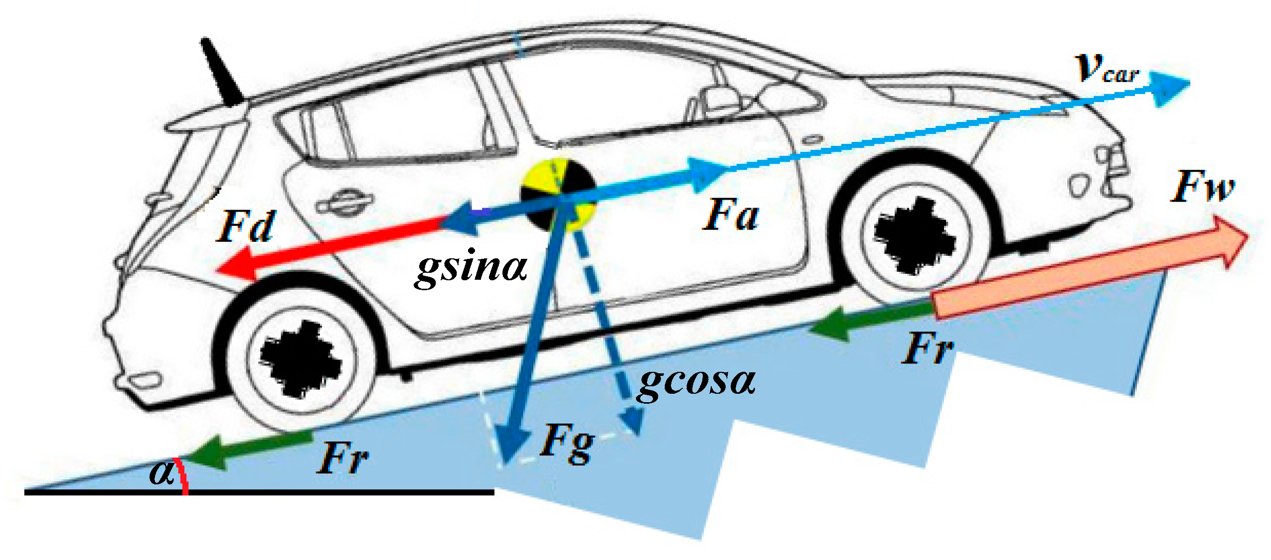
2.1. The Force Model

This section will explain the energy consumption and analysis of the power train load levels, and it’s assumed that the car body is solid, and therefore it can be modeled as a grouped mass at the center of gravity of the car [29]. Moreover, the dynamics in only one direction, which is the forward longitudinal direction, are of importance while assuming that the stability of the car does not violate under any circumstances. According to the principle of forces balance contained in Newton’s Second Law’ of mechanics, the dynamic movement of a car in one completely coordinated axis is determined by the sum of all forces operating on it in the same direction axis, as shown in Figure 2.
The tractive force, Fwheel, which must come to the wheels from the electrical machine, must overcome the sum of all the resistance forces influential on the car which are: force due to aerodynamical drag, Fd, tires rotation resistance, Frr, acceleration force, Fa, and gradient force on road, Fg. The traction force of a vehicle can be described as in [30]:
F w h e e l = 1 2 ρ F d A   v c a r v w i n d 2 + m g   c o s α F r + m g   s i n α + m a
where Fwheel, power train shaft wheel force, ρ, dry air density at 20 °C, Fd, aerodynamically drag factor, A, cross-sectional area (the car front area), vcar, car longitudinal speed [m/s], vwind, the headwind speed [m/s], m, the equivalent mass of the car, g = 9.81, gravitational constant [m/s2], α, [rad] angle of the road inclination (road slope), Frr, wheel rotation resistance factor, α = d d t   v t , car acceleration [m/s2].
Rotation resistance occurs due to many different influences that occur around and inside the car’s tires through the rotation. The rotation resistance factor depends on tire pressure, linear speed, road phenomena, road surface type, and car tires. One of the main influences is that the repeated tire deviation causes a slowdown within the tire material, resulting in an internal force that resists movement [31], and the direction of this force opposite the direction of movement, and the value is directly proportional to the gravitational force factor. The rotation resistance depends on more than seven different influences, which makes estimating the rotation resistance by analytical modeling very complicated in [29], so, the factor of rotation resistance, Frr, is expressed in [32] as follows:
F r r =   0.01 1 + 3.6 100   v c a r
where 3.6 is the velocity conversion unit (the kilometers traveled within one hour).
Figure 3 shows the different velocity dependencies available for Frr in [33,34], both of which assume that they typically depend on available tire measurements. The marks from Bosch symbolize tire design velocity limits: 180 km/h for S, 190 km/h for T, 210 km/h for H, 240 km/h for V, 270 km/h for W, above 240 km/h for Z, and finally, ECO tires are low-roll resistant tires specially designed to reduce tire rotation energy, which reduces the required rotation effort, that comes in various speed ranges. Also, Figure 3 usually illustrates three analytic expressions: one is linear [30], one that is weakly dependent on the velocity square [31], and one that is strongly dependent on the velocity square [29]. It can also be observed that Frr increase with velocity is somewhat smaller for tires with a lower velocity rating and that Frr is slightly larger compared to tires with higher velocity ratings. In [35], based on manufacturer datasheet for new tires from 2005, the average Frr for low-velocity tires (up to 180–190 km/h) is 0.0098 for high-velocity tires (up to 210-240 km/h) is 0.0101, in whereas high-velocity tires (greater than 240 km/h) are 0.0113. Both acceleration and gravitational forces are the product of car mass, and consequently, it follows that a given acceleration level for any car causes the same force of the wheel as a certain level of the road gradient as shown in Table 3.
In the state of a road gradient (or slope), car dynamics will be influenced by the gravitation force factor Fg parallel to the road.
α   =   r i s i n g d r i v i n g   =   g r a d i e n t   % 100  
where α is the angle between a road gradient and the horizontal plane (rad/s) while the rising is the vertical axis and the driving is the horizontal distance as shown in Figure 2. The road inclination is often expressed as a percentage of gradient %. The mechanical power, Pw, that must come to the wheels, from the power train required to drive a car at speed v, is the product of the wheel force and velocity of the car as follows:
P w = F w · v s
The total energy of the wheels expended while driving, dEw, is as follows:
d E w = F w · v 2 s
Meanwhile, the car may move up or down, these forces may be resistant or contribute to the net traction force on the car, meaning that it will be either negative or positive. Thus, driving on an uneven road will cause temporary storage and drain the energy inherent in the car. Still, passenger cars are commonly temporarily displacement for only a day or so, from the starting point (home for example), regardless of the path they took, the potential energy remains the same when returning to the starting position. Whereas, BEV is usually able to recover some energy from going down as it is with deceleration. For each time step, you must pay attention to the wheel force tick to calculate propulsion, braking, and power separately.

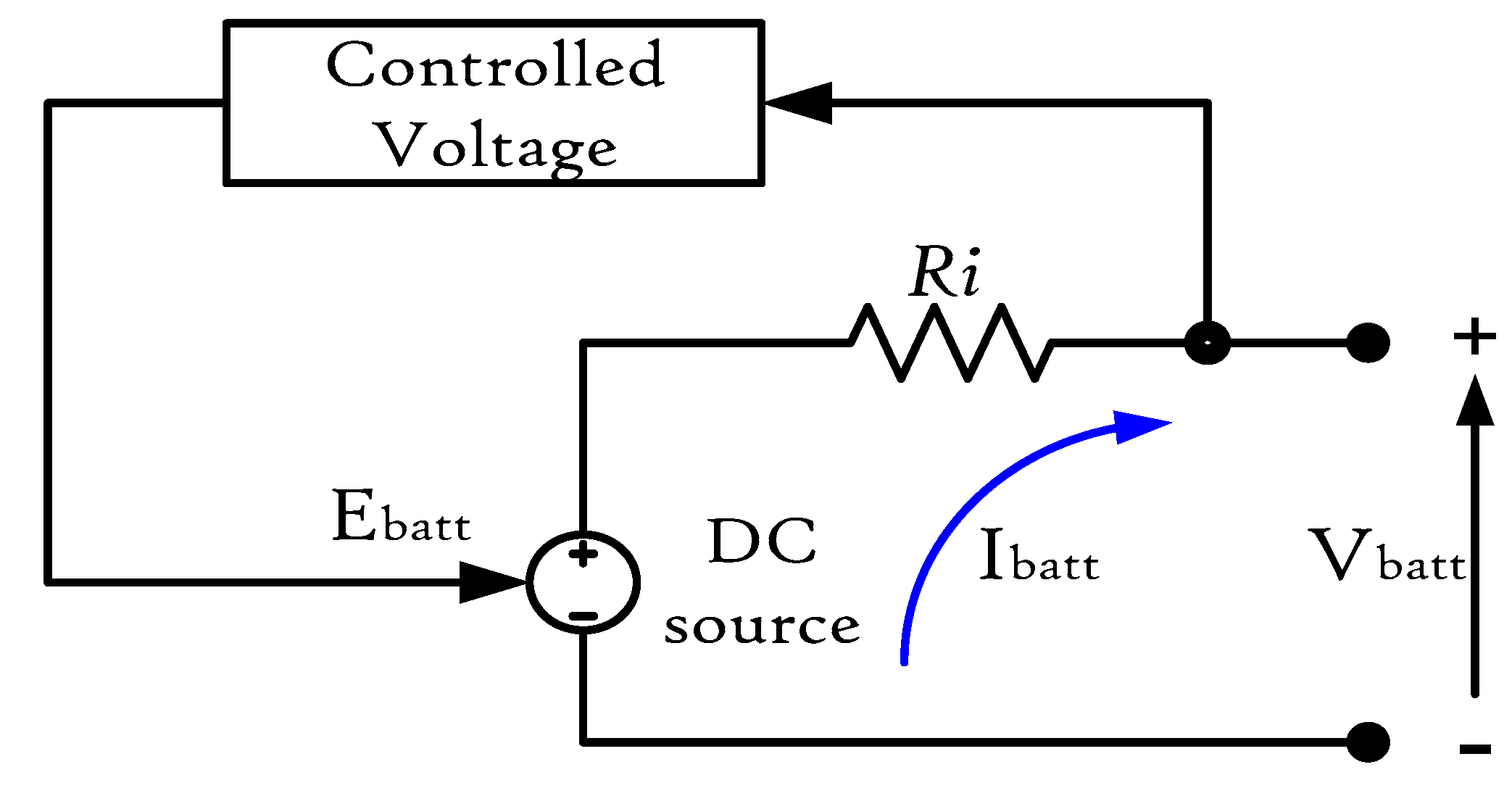
2.2. The Battery Model

The battery is the heart of electric cars. There are many different types of batteries, for example, lead-acid, nickel-metal hydride, lithium-ion, etc. The type of battery selected on this sheet was Li-ion battery: this category belongs to the family of rechargeable batteries. The lithium-ion battery is the preferred choice due to its relatively specific power, also its strength to deal with the harsh operating environment that it undergoes in BEV [36]. The battery was designed using a simple controlled voltage source in a series with a fixed resistance, as shown in Figure 4. Internal resistance is presumed to be fixed for simplicity reasons, though it may usually change depending on the value of the battery current or the charge and discharge status.
The circuit equivalent loop that holds the Kirchhoff voltage law is proven to produce a terminal voltage expressed as:
V b a t t = E b a t t R i I b a t t
where Vbatt is the battery voltage (V), Ebatt is the no-load voltage (V), Ri is the internal resistance (Ω), Ibatt is the battery current (A). As V and Ri depend on the charging status of the instant battery. Internal resistance Ri can be expressed as a function of battery charge and operating temperature as well as certain charge and discharge currents.

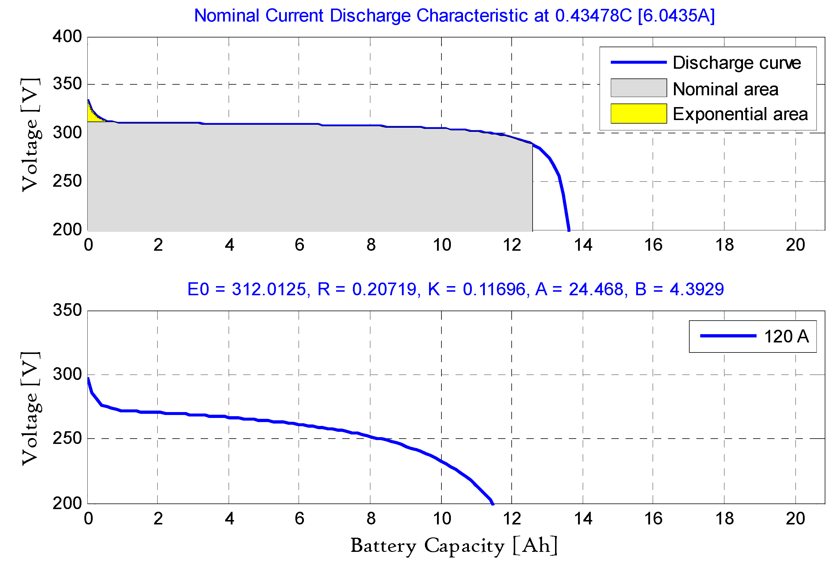
2.3. Extracting Model Parameters

The model can accurately represent the behavior of many types of batteries, provided the parameters are well defined. The main advantage of this battery model is that it is easy to draw parameters from the manufacturer’s discharge curve. Figure 5 shows the computed discharge curve typically for (Type Li-ion battery: 288 Volt 120 Ampere-hours) and is an indicator of battery voltage versus elapsed time during discharging. The fixed current used to discharge the battery is 6 Amperes (0.4C), determined by the nominal amplitude of the battery divided by one hour [37].
The battery model has been validated by specifying battery parameters, to reproduce the behavior of the LiFePO4 (3.2 V/20 Ah) battery, a real commercially available device (Li-ion battery commercial datasheet available at “https://www.ev-power.eu” accessed on 4 January 2020). Through the manufacturer’s data sheet and model output characteristics, represented by the discharge curve plot. The controlled voltage source is described by the main equations for the general battery model for a Li-ion battery as:
  • Charging phase:
    E c h g = V c K Q i t + 0.1 Q + A e B i t
  • Discharging phase:
    E d i s = V c K Q Q i t + A e B i t
where Vc is the fixed battery voltage (V), K is the polarization voltage (V), Q is the maximum battery capacity (Ah), it is the extracted capacity (Ah), A is the exponential area capacity (V) and B is the exponential area time constant inverse (Ah)−1.

2.4. Sizing Battery Pack

The battery pack sizing method depends on a predetermined minimum for all-electric range and power required by the electric motor to drive the car from initial acceleration to a fixed speed. Meantime, battery-pack operational variables such as voltage, maximum charging, discharging current, and power are related to chemistry within individual cells. The cells are connected in series and/or parallel configurations to provide the required voltage, power, and energy. The main parameters involved in battery sizing include:

2.4.1. Battery Pack Power

If the car is a battery-powered electric vehicle, all of the power sources comes from the electric motor and the battery, battery power can be obtained by:
P b a t t = P w η m o t o r
where Pbatt is the maximum battery power in kW, Pw is the wheel power, and ηmotor is the efficiency of the electric motor.

2.4.2. Specific Battery Energy (SEbatt)

The amount of energy per unit of the battery mass is called the specific energy of the battery. This parameter is a condensed property of the battery system and is expressed in watt-hours per kilogram (Wh/kg). The actual energy that can be extracted from the battery system depends on several factors such as temperature and discharging rate. As a general expression, the battery’s specific energy is:
S E b a t t = E d i s M b a t t
where Edis is the discharging energy, and Mbatt is the total battery mass. Since the discharging energy varies with the battery discharging rate, the specific battery energy also varies accordingly.

2.4.3. Battery Specific Power (SPbatt)

The specific power of the battery system is the parameter that specifies the amount of energy that can be obtained per unit mass, expressed in watts per kilogram (W/kg), and is determined by:
S P b a t t = P d i s M b a t t
where Pdis is the discharging power, and Mbatt is the total battery mass. This parameter also works as an approximation to the available power level of the battery system.

2.4.4. Battery Pack Capacity

The battery system can measure the amount of free charging produced by the active substance in the cathode and consumed by the anode. The battery capacity is calculated by the intrinsic properties of the battery cell design.
C b a t t = P b a t t R P / E
where Cbatt is the maximum battery capacity in kWh, and RP/E is the ratio of the specified power (kW) to the specified energy (kWh) of the battery.

2.4.5. Maximum Battery Pack Storage

The maximum battery storage is determined by the car’s entire electric range and the electrical consumption in the electrical model (Equation (13)). For BEV, the charge exhausting mode corresponds to the entire electric range.
E b a t t e r y   p a c k = C e l e c t r i c R A l l e l e c t r i c 0.8
where Ebatt is the maximum battery energy storage in kWh, Relectric is the fully electric range of the vehicle in km, and Celectric is the electric consumption during the fully electric operating in Wh/km. The denominator constant of 0.8 in the equation depends on the design of the state of charge (SOC%) control logic of 20% used for most battery systems [38,39].

2.4.6. Efficient Battery Power

Battery energy efficiency is defined as the percentage of electrical energy that is connected by a battery from a particular charge state to the energy required to return the battery to the same charge condition. Although battery efficiency is not a clear parameter for measuring battery performance, it is effective as a comparative measure of different power and energy management strategies. If using the battery management system operates the battery by reducing high energy quick discharges, the battery efficiency is expected to increase compared to the battery operation without a management system. In the case of a pure electric vehicle, a comparison should be made based on the battery charger profile itself. The battery discharging energy (Edis) can be expressed as a function in the discharging time tf, open-circuit voltage Voc, the internal resistance Ri and the current constant discharging Id as:
E d i s = 0   t f   P d   t d t = t f V o c I d R i I d
Charge the battery for the same discharging period tf, the same as the magnitude of charging current, as the discharging current gives the charging energy (Echg) as:
E c h g = 0   t f   P d   t d t = t f V o c + I d R i I d
Therefore, the battery efficiency expressed as a function of the current battery can be indicated as:
η b a t t = E d i s E c h g = V o c I d R i   V o c + I d R i  

2.4.7. Battery Cell Numbers

Battery cells must be placed in series and parallel to meet voltage and power needs. Particularly, strings rank in a series can lead to increased voltage and resistance while strings rank in parallel can lead to increased energy capacity.
N s e r i e s = V p a c k V c e l l     ,   N p a r a l l e l = E p a c k E c e l l
where Vcell and Vpack are the battery cell voltages and pack, Ecell and Epack are the battery cell energy capacity and pack, Nseries is the number of series cells, and Nparallel is the number of parallel cells.
The studied 288 V/120 Ah battery bank is composed of six-packs in parallel, and every pack is made up of 6 × 48 V/20 Ah modules in series. The specifications are listed in Table 4.

2.5. Monitoring and Estimating the Battery SOC

The state of charge (SOC) indicates the remaining battery capacity. SOC units are percentage points (0% = empty, 100% = full). SOC is usually used when discussing the current state of the used battery. SOC rating can help determine thresholds for each battery operating mode (i.e., charge or discharge) and overcharge and over-discharge can also be avoided. SOC is expressed as:
S O C t = Q 0 t i t d t
The state of discharge (SOD) is defined as the charge gauge derived from the battery, as:
S O D t = q = 0 t i t d t
The depth of discharge (DOD) is the inverse of SOC (100% = empty, 0% = full), one on SOC. DOD is often seen when discussing battery life after repeated use.
D O D t = 0 t i t d t Q 100 % =   S O D t Q 100 %
The state of health (SOH) is the battery status today compared to its ideal state. The SOH units are percentage points (100% = new battery). By detecting SOH, the battery life and health status can be estimated and the percentage of battery life can be used to determine whether or not it will be replaced.

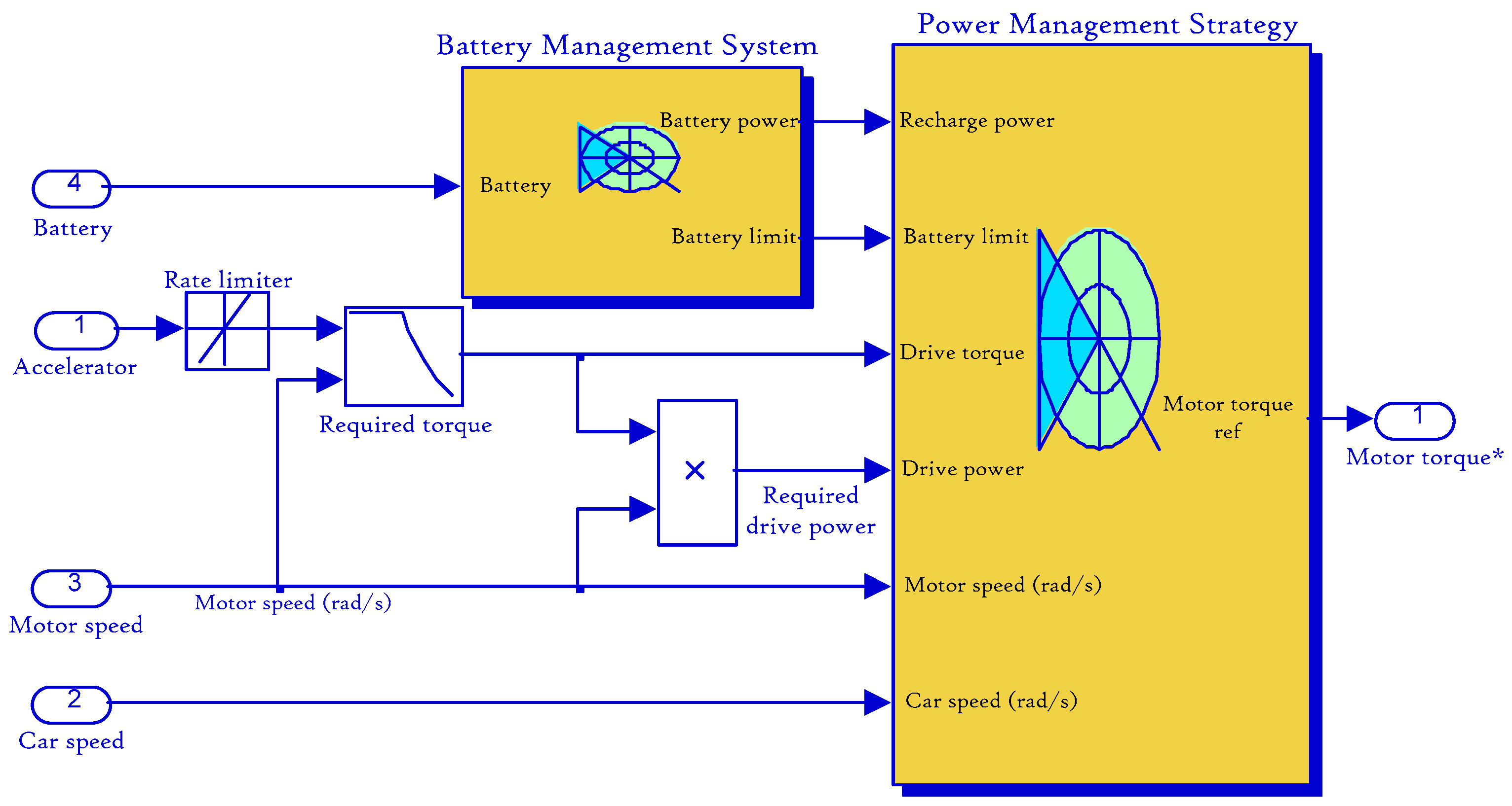
3. Energy Management Strategy

The EMS is responsible for distributing energy between multiple energy systems in light of the vehicle’s continuous energy requirements, as shown in Figure 6. Then the EMS task is to implement decision-making rules and restrictions for generating this energy distribution and recovery orders or actions. All simulations started with the battery charged to 95% of its energy capacity, as a margin of a few percent is typically used in BEVs to prolong the battery lifetime. Figure 7 demonstrates the energy management strategy in the Simulink model.
The energy management strategy (EMS) corrects DC bus load disturbances in a low time horizon. Indeed, the horizon period is the EMS decision era, and it is time-limited to generate reference power paths. Figure 8 shows battery power limits (Pbatt max, Pbatt min) and power rate limits (dPb/dt) as a function of battery charge status. In graphs (a) and (b), the battery discharging power limit and battery charging limit, respectively, (∆EMS) represent the charging and discharging power limits during a specified period of EMS decisions. Consequently, the inclusion of these restrictions in the definition of EMS allows control of step-change for both charging and discharging levels.

3.1. Battery Management System

The old battery management systems (BMS) do not include a power control unit. Advanced battery technologies such as lithium-ion require a power control unit to ensure the safety and long-term performance of the battery pack. The suggested power control unit also controls battery recharging by forwarding recovered energy (i.e., regenerative braking) to the battery pack as shown in Figure 7. The suggested power control unit will also work on:
1.
Fully protect the battery from damage.
2.
Monitor cells, units, and packages to ensure that they operate within the appropriate range and avoid faulty operation such as short circuits, overvoltage, overcharging, over-discharging, and overheating of particular importance to Li-ion cells.
3.
Ensure safe operation and extend battery life for as long as possible.
4.
Communicate with the supervisor of the vehicle and meet all the requirements for operating the vehicle.
5.
Balance cell groups during dynamic charging and discharging to ensure that the entire battery system provides optimum performance.

3.2. Power Control Unit Suggested
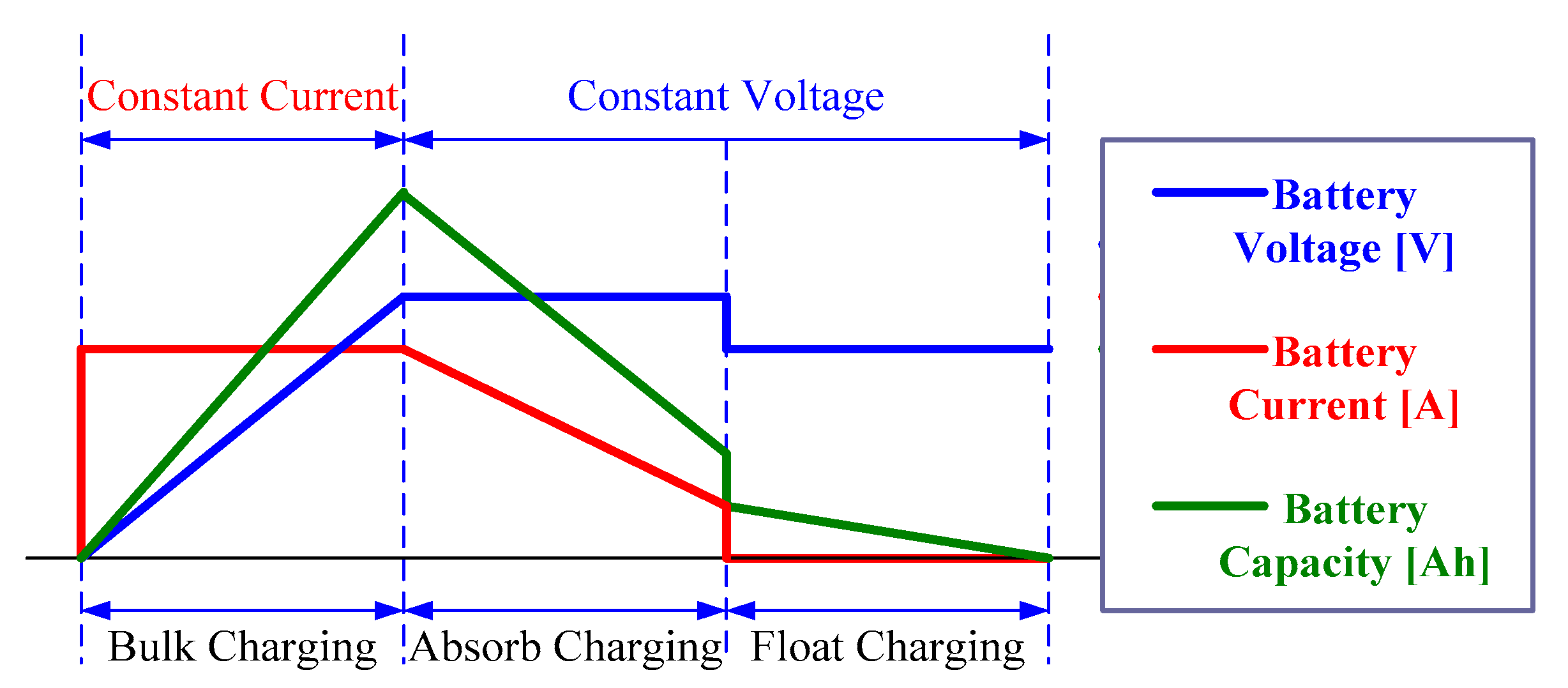
The main function of the suggested power control unit is to connect and disconnect the battery from the load or the charger. It also measures the current and voltage of the battery pack and limits the flowing current in [40]. Figure 9 shows a schematic diagram of the suggested power control unit. The power control unit model relies on the battery pack specifications that monitor its status, calculating secondary data, report that data, control its environment, authenticate, and balance it.
For lithium-ion batteries are the main energy storage units for BEVs, these batteries must be able to handle random charges due to regenerative braking. The regenerative braking force can reach a 10 kW level. Safety limits must be applied to ensure the optimal and safe operation of the battery pack. The constant-current constant-voltage (CCCV) charge technique is the charge profile recommended by most manufacturers of lithium-ion batteries [41]. Figure 10 shows the charge profile for a single Li-ion battery cell. The three most common stages are charge, discharge, and standby. These stages can also be summarizing below.
In Stage 1: (Charging Mode), this mode works when the EMS orders the battery to be charged. This mode can include a power level, in which case the charge current is controlled to deliver the required power. Also, a different charging strategy is determined depending on the SOC of the batteries. Figure 10 shows a diagram of the three battery charging strategies as follows:
(1)
Bulk charging mode or CC charge (current control)—used for fast charging when the SOC is low, where the charger current is kept at a steady rate, and the battery voltage is enabled to grow accordingly during recharging.
(2)
Absorption charging mode or CV charge (voltage control)—used to prevent battery overcharging when the SOC is higher than a certain level.
(3)
Float charging mode (voltage control)—used when the battery is close to full charge and maintains the full charge state of the battery.
In Stage 2: (Discharging Mode), this mode works when EMS orders the power storage device (batteries) to discharge. In this mode, the discharge current is controlled to deliver the required power. There are two factors that EMS should consider: (a) the energy capacity of an electrochemical battery decreases at a higher discharging current [42,43]; and (b) a minimal SOC is often required during discharge to increase the life of the cycle [44,45].
In stage 3: (Standby Mode), the system usually enters into standby mode when charging ends when the maximum SOC is reached. In this mode, the battery pack is still attached to the system but is not significantly charged or discharged. For the electrochemical battery, float charging can be used to compensate for the self-discharging [46,47,48,49,50,51].

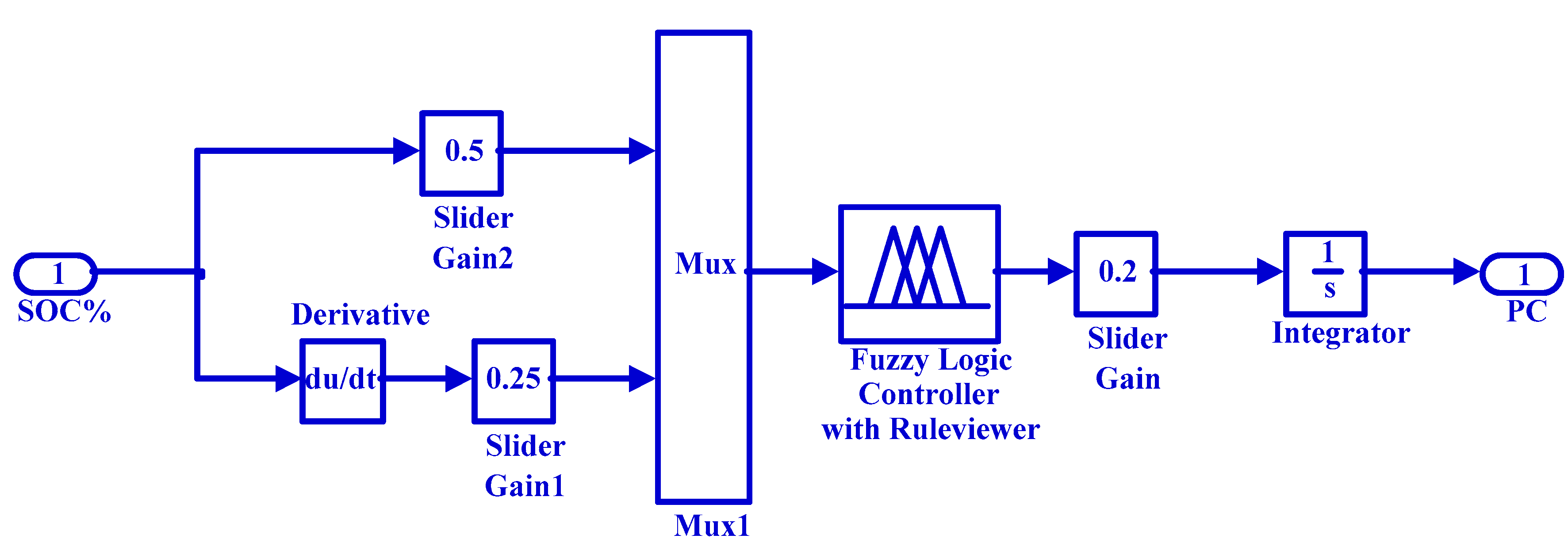
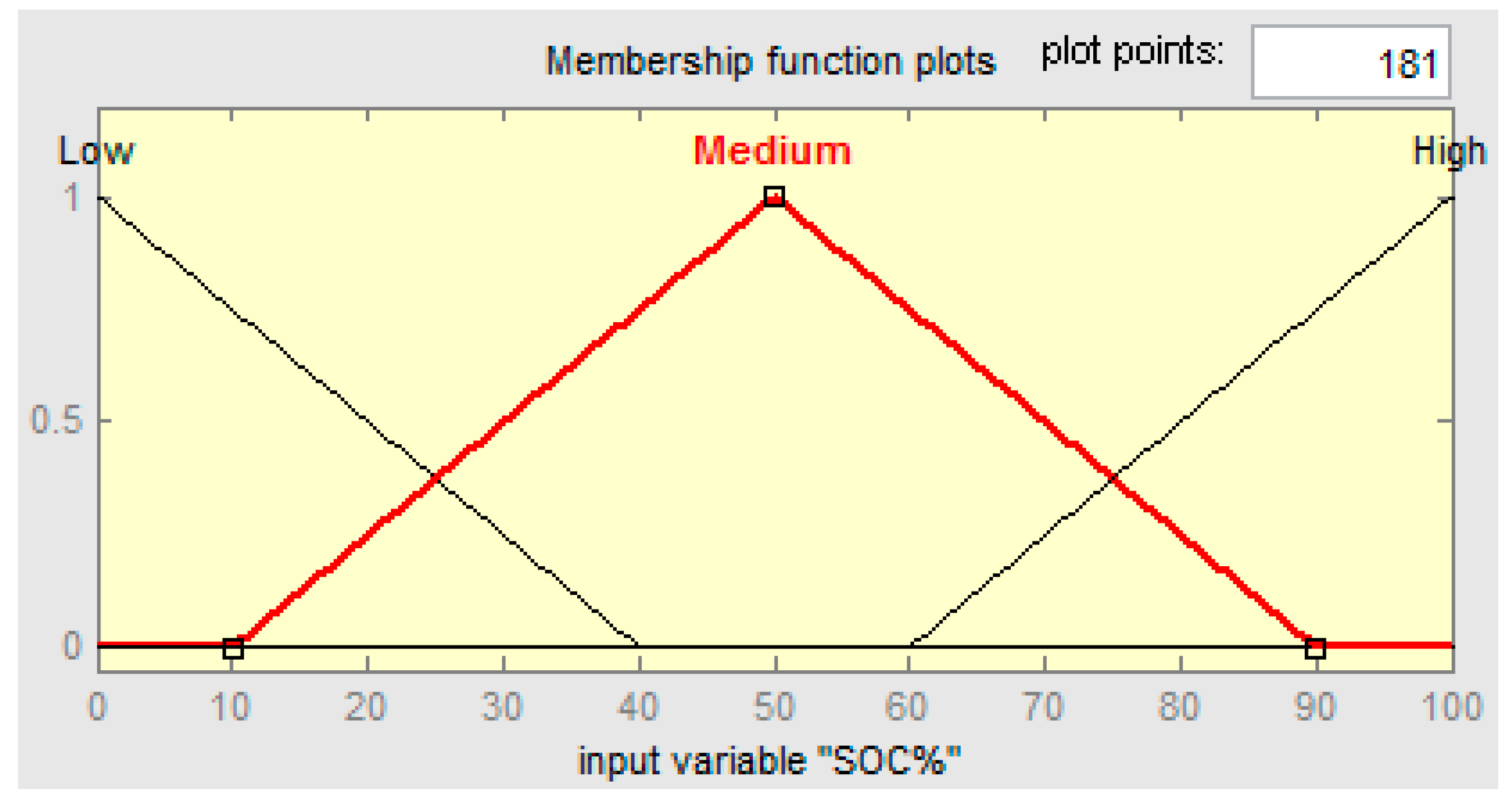
3.3. Suggested Fuzzy Logic Controller

Fuzzy logic control is used as a strategy implementation tool, Figure 9. First, the input variables and output variables of the FLC have to be defined, then a set of fuzzy rules suitable for the control strategy can be created. The main objective of BMS control is to improve the battery operating point and electric motor through efficient operation, reliability, and high power quality of the power train. This is done by controlling charging and discharging limits utilize FLC. Thus the electric motor operation should be adjusted according to the battery charging state (SOC) and current road load. As shown in Figure 9, the input variables for the power control unit are the SOC of the battery, voltage state, and current at the node to which it is connected. If the SOC battery charge state is low that is (less than 20%) and the node voltage is high, the EV battery will be charged, but if the SOC battery charge state is high that is (greater than 80%) and the node voltage is lower, the EV will be discharged. Also, there are several different conditions where both the SOC and the node voltage can be low or both are high. In these situations, specified charging and discharging rates are employed. Thus, to keep node voltage changes within standard rates, FLC should be adjusted to monitor such other conditions also. Figure 11 provides a schematic diagram of an FLC.
Second, the functions of the individual membership and the fuzzy sets of FLC are determined based on the fuzzy expert knowledge system to more accurately reflect the status of the input and output variables. Each membership function consists of some fuzzy sets. A fuzzy set is a set of values related to fuzzy input. Each element of the fuzzy set contains real values that range in varying degrees between 0 and 100%, as shown in Figure 11, known to be the degree of their membership within the set. Also, the symmetric triangle function was chosen because it provides good results and has better transition performance and calculations using these simpler shapes. E.g., affording to a battery expert, the battery state SOC membership function is divided into three levels, high SOC (>80%), medium SOC (40–80%), and low SOC (<40%), each value represents a fuzzy set. Figure 12 below shows the battery SOC% membership function.

3.4. Adaptive Neural Fuzzy Inference System

FLC relies fundamentally on the fuzzy expert knowledge system based on the description included in Section 3.4, and thus it cannot achieve satisfying efficiency permanently. So ANFIS theory will be used to improve membership functions and FLC rules after training ANFIS with actual driving cycle data for better efficiency [44,45]. This paper aims to save energy by a specific path. Figure 13 illustrates the adaptive neural fuzzy inference system (ANFIS) consisting of two inputs in a general form of common rules and one output. The method of adjusting the fuzzy logic control within ANFIS has five layers as shown in Figure 13.
Simulating ANFIS requires five main steps, as follows:
(1)
Obtaining training data of different driving cycles, each driving cycle is characterized by different road modes, and partial samples of NEDC and UDDS driving cycles are selected in the simulation of ANFIS training to achieve the improved FLC. In simulations, points 0–100, 500–600, 1000–1100 of the different driving cycles are determined as samples.
(2)
Use the data to train ANFIS.
(3)
Get new membership functions.
(4)
Obtaining the new FLC block in the MATLAB.
(5)
Obtain simulation results.
where x1 and x2 as status input variables and Yi representing the output variable, Ai are the input membership functions, Ψi are the rules firing strengths, as follows:
  • Rule 1:
    IFx1isAiANDx2isBiTHENYi = Ψi (x1, x2)
  • Rule 2:
    IFx2isAiANDx2isBiTHENYi = Ψi (x1, x2)
Using (Pbatt max) as the output function’s fuzzy inference system, the rule instance for creating a fuzzy base rule as:
FISIF speed is fast AND battery SOC is high THEN Pbatt max = Pbatt max
By recursive calculation of each rule, the fuzzy logical output variable Pbatt is evaluated as the maximum output, where Aij is the combined membership function which is evaluated as:
P b a t t   m a x   = i = 1 i m a x j = 1 j = 2 A i j ( x j ) Ψ i i = 1 i m a x j = 1 j = 2 A i j ( x j )

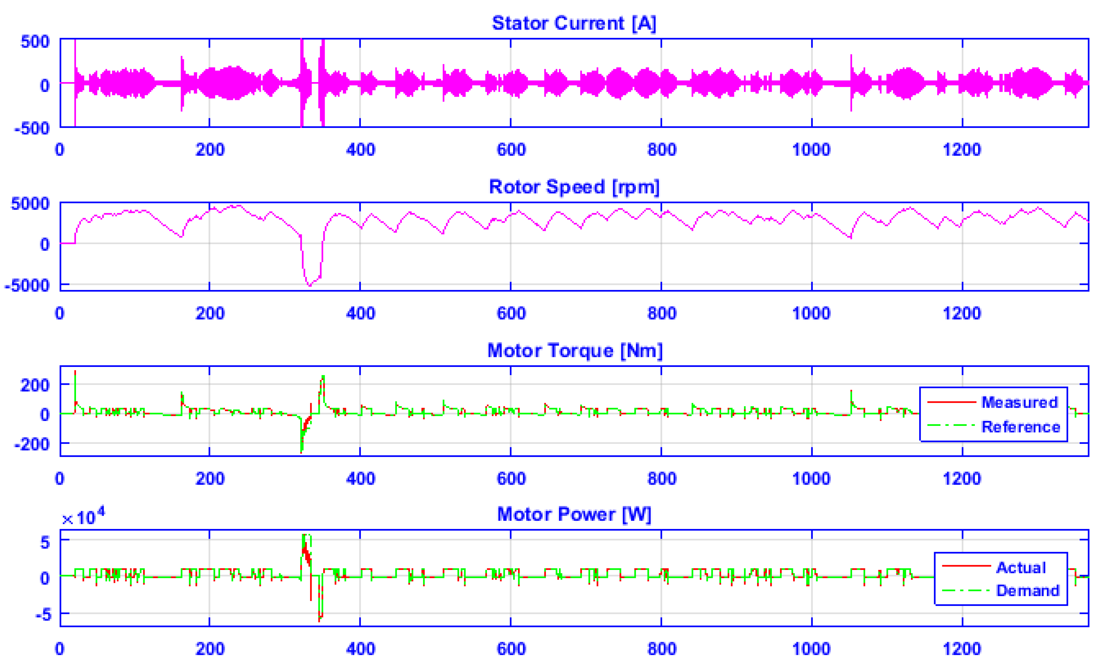
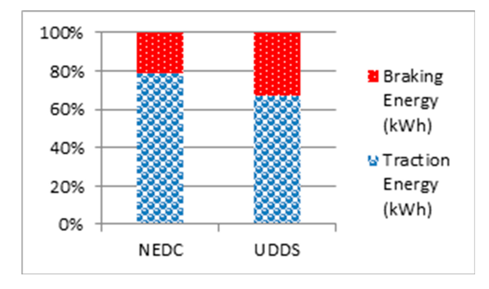
4. Results and Discussion

The battery-powered electric vehicle model is shown in Figure 6 by applying the detailed mathematical models of the system described earlier in the MATLAB/Simulink® environment. Simulation results are obtained based on typical driving cycles. Different driving patterns and situations have been chosen to assess the performance of the proposed EMS to define typical driving patterns on different types of roads. In this paper, two different driving cycles were simulated: NEDC and UDDS. Figure 14 shows simulated car results for 20 s (a) car speed, (b) battery power, (c) battery voltage, (d) battery current, and (e) battery charge status (%), respectively. The electric car starts to operate from the stop position at the time (t = 0), and the car is suddenly pushed to 70% of the vehicle’s acceleration. After about (t = 0.8 s), the power required for the car reaches about 10 kW. The brakes are pushed to 70% at the time (t = 8 s), which causes the electric motor to convert the brake energy using the regenerative braking method, the energy is stored again in the battery and charged for (t = 8 s). After that the accelerator is suddenly pushed back to 70% at the time (t = 16 s), thus it is observed that the battery power and current decrease are slowly until the battery reaches the value of the initial charge state.
The simulation results performed under the accelerated braking cycle revealed in Figure 14, Reveal that FLC gives a 35% increase in the fundamental output with improved quality (i.e., less THD compared to PI) and that the resulting THD was 1.564% for PI, versus 0.552% for FLC. FLC results also showed good and high performance in time domain response, and the effect of rapid perturbations rejection on the system compared to the charts in the literature. Thus, the core loss of PMSM greatly reduces, thus improving the efficiency of the drive system.
The results obtained are tabulated as a comparative performance in light of the settling time and peak overshoot, as shown in Table 5. The outputs of the conventional proportional integrated control (PI) system have a very high overshoot and settling time. The enhanced fuzzy logic controller (FLC) has a better settling time and lower overshoot.

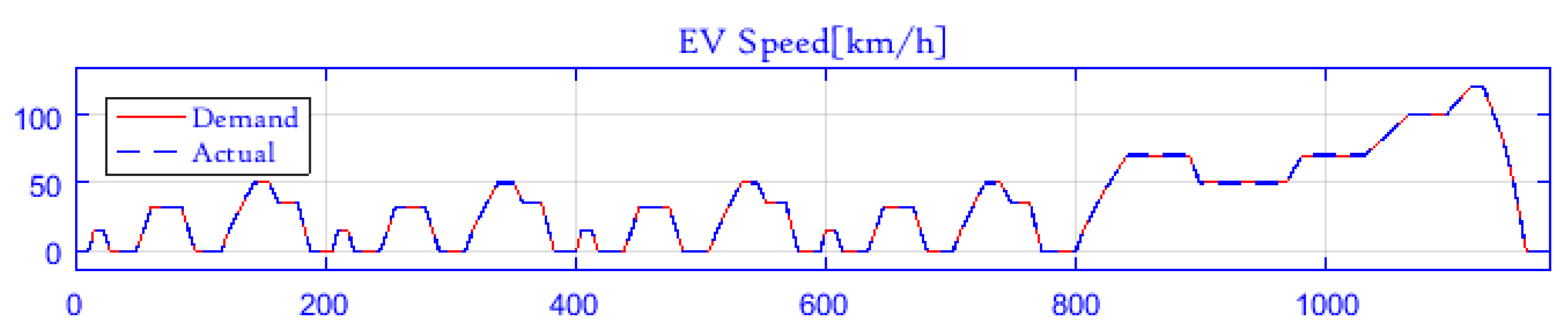
4.1. Description of Driving Cycle NEDC

The driving cycle is a series of points representing the car’s speed against time, to calculate the car’s efficiency (Energy Saving). The New European Driving Cycle (NEDC) consists of four ECE-15 repeated driving cycles and an (Extra-Urban Driving Cycle) or EUDC to simulate highway driving in a vehicle. NEDC driving cycle operates at a distance of 11 km per hour approximately in 1180 s and has an average speed of 33.6 km per hour, as shown in Table 6. During this cycle, the SOC of the battery pack almost decreased to 50% from 70% of the initial SOC. The frequent start and stop characteristics of city driving were more suitable for energy recovery using regenerative braking. Simulation results show that the car was able to meet the driver’s requirements, as it can be seen that the demand and actual speeds of the car were identical. Figure 15, Figure 16 and Figure 17 show graphs of the demanded and actual speeds of the NEDC driving cycle simulator, along with the plots of the motor, and the battery. The entrance to the simulation will be the repeated NEDC 15 times as this should provide a drive distance of 165 km which should be acceptable.

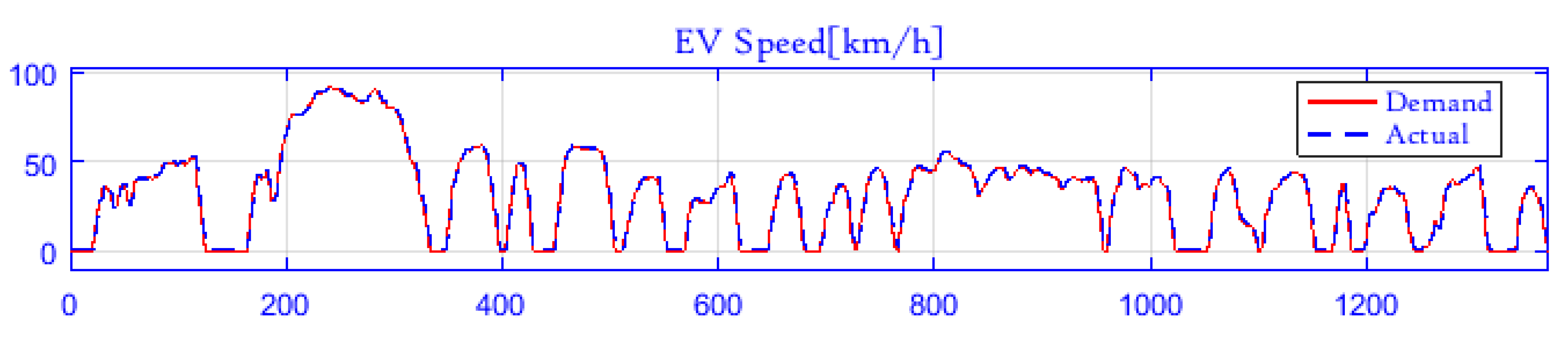
4.2. Description of Driving Cycle UDDS

The Urban Dynamometer Driving Schedule (UDDS) driving cycle aims to simulate city driving conditions that are used to test light vehicles. UDDS driving cycle operates at a distance of 12 km per hour approximately 1369 s and has an average speed of 31.6 km per hour, as shown in Table 7. During this cycle, the SOC of the battery pack almost decreased to 45% from 70% of the initial SOC. Simulation results show that the car was able to meet the driver’s requirements, as it can be seen that the demand and actual speeds of the car were identical. Figure 18, Figure 19 and Figure 20 show graphs of the demanded and actual speeds of the UDDS driving cycle simulator, along with the plots of the motor, and the battery. The entrance to the simulation will be the repeated UDDS 15 times as this should provide a drive distance of 180 km which should be acceptable.
A reduction in traction energy demand can be observed when moving from NEDC to UDDS, while brake energy increases by 21.8% as shown in Figure 21, which shows more opportunities to exploit regenerative braking.

5. Conclusions

In this research, an energy management strategy was conducted for electric vehicles in MATLAB/SIMULINK environment. The electric car battery is chosen in a way that meets the power and energy requirements of a specific driving cycle. The loss of every component in the car depends on the interior conditions of the car, such as voltages, currents, speed, torque, and charge/discharge status. The battery good fuzzy logic control is set up and is the basis for the power management controller in the same battery management system. The results show that EMS tested vehicle strategies can achieve, in nearer-reality test conditions such as those for NEDC, higher efficiency levels than those currently evaluated in UDDS. This model also helps to develop the PMS system, which controls all adapters in addition to the PMSM motor, so that it does not exceed the maximum battery power. Finally, it is possible to precisely control the charge and discharge of the battery.
The driver can choose the operating mode (energy-saving) using the graphical user interface or device selector. Moreover, the benefits of the proposed EMS and its control strategy can be summarized as follows:
1.
Simulation results showed better performance of the proposed adaptive FLC over conventional PI control.
2.
Adaptive FLC introduced an effective solution to correctly EMS.
3.
Using adaptive FLC, much better results can be achieved due to lower harmonic current and thus torque ripple less than conventional PI.
4.
Several tests were performed using simulations to analyze harmonic components for speed. All THD values are less than 5%, which is acceptable harmonic distortion according to the IEEE standard.
5.
Finally, adaptive FLC offers very good speed control performance.

Author Contributions

Conceptualization, H.S. and K.S.; methodology, A.K.; validation, K.S., A.S.A. and A.G.A.-K.; resources, A.S.A.; data curation, A.G.A.-K.; writing—original draft preparation, H.S.; writing—review and editing, H.S. and K.S.; supervision, A.K. All authors have read and agreed to the published version of the manuscript.

Funding

This research received no external funding.

Acknowledgments

The author would like to thank Deanship of Scientific Research at Majmaah University for supporting this work through research group No (RGP-2019-19).

Conflicts of Interest

The authors declare no conflict of interest.

Nomenclature

ANFISAdaptive Neural Fuzzy Inference System
BESSsBattery Energy Storage Systems
BEVs Battery Electric Vehicles
BMS Battery Management System
CCConstant Current
CEVsCombustion Engine Vehicles
CVConstant Voltage
DCDirect Current
DGDistributed Generation
DODDepth of Discharge
ECE-15European Standard Urban Driving Cycles
EGVElectric Ground Vehicle
EMSEnergy Management Structure
EUDCExtra-Urban Driving Cycle
EVElectric Vehicle
FLCFuzzy Logic Controller
HEVs Hybrid Electric Vehicles
ICEInternal Combustion Engine
IGBTsInsulated Gate Bipolar Transistors
Li-ionLithium-Ion
LPVLinear Parameter Variable
LQRLinear Quadratic Regulator
MGsMicro-Grids
NEDCNew European Driving Cycle
PHEVsPlug-in Hybrid Electric Vehicles
PIProportional Integral
PIDProportional Integral Derivative
PMSPower Management Strategy
PMSMPermanent Magnet Synchronous Motors
PMUPower Management Unit
PSOParticle Swarm Optimization
RERsRenewable Energy Resources
SOCState of Charge
SODState of Discharge
SOHState of Health
THDTotal Harmonic Distortion
UDDSUrban Dynamometer Driving Schedule
UUGUpstream Utility Grid
List of Notations
SymbolDescription
aAcceleration (m/s2)
AThe cross-sectional area of the vehicle (m2)
BpkThe peak flux density in the B-H hysteresis curve
CdAerodynamic drag coefficient
d,qDirect, quadrature axis components
EdDrag energy (W)
EgGravitational energy (W)
EkKinetic energy (W)
Eon+offThe energy dissipated during turn-on and turn-off (W)
ErRolling energy (W)
ErrThe energy dissipated during turn-off (due to the reverse recovery process) (W)
EtThe total energy of the section (W)
fFrequency of the flux
FaAcceleration force (Nm)
FdDrag force (Nm)
FgGravitation force (Nm)
FrRolling force (Nm)
FresistiveThe sum of the resistive forces acting to decrease the vehicle speed (Nm)
fswSwitching frequency
FtractiveThe sum of all the tractive forces acting to increase the vehicle speed (Nm)
FwTractive force (Nm)
gGravitation constant (m/s2)
IIGBTThe average current (A)
kCoupling coefficient
KThe scaling constant for transformation between three-phase to two-phase space vectors
kcEddy current parameter
khHysteresis parameter
Ld, LqThe d- and q-axis winding inductances
LmMutual inductance of three inductors (mH)
mVehicle mass (kg)
nDepends on Bpk, fr, and steel material (typically 1.6-2.2)
npNumber of pole pairs
PaUnit of standard atmospheric pressure (Pascal)
rWheel radius (m)
RcCore loss resistance (Ω)
RCEIGBT on-state resistance (Ω)
RFdiode on-state resistance (Ω)
RL_acAC load resistance (Ω)
RL_dcDC load resistance (Ω)
RsStator winding resistance (Ω)
TNo.Number of turns per inductor
v(t)Vehicle speed (m/s)
VbattBattery voltage (V)
vcarVehicle speed (m/s)
VCEThe IGBT threshold voltage of the on-state characteristics (V)
vwindWind speed (m/s)
wWheel speed (rad/s)
welThe electrical angular speed (rad/s)
wrThe rotor angular speed (rad/s)
αRoad inclination angle (rad/s)
ρAir density (kg/m3)
Ψd, ΨqFlux linkage in the d- and q-axis
ΨmFlux linkage related to the permanent magnet

References

  1. Rahman, K.M.; Patel, N.R.; Ward, T.G.; Nagashima, J.M.; Caricchi, F.; Crescimbini, F. Application of direct-drive wheel motor for fuel cell electric and hybrid electric vehicle propulsion system. Ieee Trans. Ind. Appl. 2006, 42, 1185–1192. [Google Scholar] [CrossRef]
  2. Mock, P. European Vehicle Market Statistics; The International Council of Clean Transportation (ICCT): Washington, DC, USA, 2014. [Google Scholar]
  3. Rajashekara, K. Present status and future trends in electric vehicle propulsion technologies. IEEE J. Emerg. Sel. Top. Power Electron. 2013, 1, 3–10. [Google Scholar] [CrossRef]
  4. Wu, X.; Freese, D.; Cabrera, A.; Kitch, W.A. Electric vehicles energy consumption measurement and estimation. Transp. Res. Part D Transp. Environ. 2015, 34, 52–67. [Google Scholar] [CrossRef]
  5. Gao, D.W.; Mi, C.; Emadi, A. Modeling and simulation of electric and hybrid vehicles. Proc. IEEE 2007, 95, 729–745. [Google Scholar] [CrossRef]
  6. Mapelli, F.L.; Tarsitano, D.; Mauri, M. Plug-in hybrid electric vehicle: Modeling, prototype realization, and inverter losses reduction analysis. IEEE Trans. Ind. Electron. 2010, 57, 598–607. [Google Scholar] [CrossRef] [Green Version]
  7. Schaltz, E. Design of a Fuel Cell Hybrid Electric Vehicle Drive System. Ph.D. Thesis, Aalborg University, Aalborg, Denmark, 2010. [Google Scholar]
  8. Wang, H.; Zhang, X.; Ouyang, M. Energy consumption of electric vehicles based on real-world driving patterns: A case study of Beijing. Appl. Energy 2015, 157, 710–719. [Google Scholar] [CrossRef]
  9. Vehicle Driving Patterns and Measurement Methods for Energy and Emissions Assessment. Available online: https://www.bitre.gov.au/sites/default/files/op_030.pdf (accessed on 8 December 2020).
  10. Fuel Economy Labeling of Motor Vehicle Revisions to Improve the Calculation of Fuel Economy Estimates. Available online: https://www.epa.gov/regulations-emissions-vehicles-and-engines/final-rule-fuel-economy-labeling-motor-vehicles-revisions (accessed on 8 December 2020).
  11. Advanced Powertrain Research Facility, Avta Nissan Leaf Testing and Analysis; Idaho National Laboratory (INL), Advanced Vehicle Testing Activity (AVTA): Idaho Falls, Idaho, 2013.
  12. Williamson, S.S.; Emadi, A.; Rajashekara, K. Comprehensive efficiency modeling of electric traction motor drives for hybrid electric vehicle propulsion applications. IEEE Trans. Veh. Technol. 2007, 56, 1561–1572. [Google Scholar] [CrossRef]
  13. Boretti, A. Analysis of the regenerative braking efficiency of a latest electric vehicle. In SAE Technical Paper; SAE International: Warrendale, PA, USA, 2013. [Google Scholar]
  14. Hayes, J.G.; Davis, K. Simplified electric vehicle powertrain model for range and energy consumption based on EPA coast-down parameters and test validation by Argonne national lab data on the Nissan Leaf. In Proceedings of the 2014 IEEE Transportation Electrification Conference and Expo (ITEC), Dearborn, MI, USA, 15–18 June 2014; pp. 1–6. [Google Scholar]
  15. An, F.; Barth, M.; Scora, G. Impacts of diverse driving cycles on electric and hybrid electric vehicle performance. In SAE Technical Paper; SAE International: Warrendale, PA, USA, 1997. [Google Scholar]
  16. de Gennaro, M.; Paffumi, E.; Martini, G.; Manfredi, U.; Scholz, H.; Lacher, H.; Kuehnelt, H.; Simic, D. Experimental investigation of the energy efficiency of an electric vehicle in different driving conditions. In SAE Technical Paper; SAE International: Warrendale, PA, USA, 2014. [Google Scholar]
  17. Zaccardi, J.-M.; Le Berr, F. Analysis and choice of representative drive cycles for light-duty vehicles case study for electric vehicles. Proceedings of the Institution of Mechanical Engineers. Part D J. Automob. Eng. 2012, 227, 605–616. [Google Scholar] [CrossRef]
  18. Neudorfer, H.; Binder, A.; Wicker, N. Analyse von unterschiedlichen fahrzyklen fur den einsatz von elektrofahrzeugen. Elektrotechnik Und Inf. 2006, 123, 352–360. [Google Scholar] [CrossRef]
  19. Qi, Z.; Shi, Q.; Zhang, H. Tuning of digital PID controllers using particle swarm optimization algorithm for a CAN-based DC motor subject to stochastic delays. IEEE Trans. Ind. Electron. 2020, 67, 5637–5646. [Google Scholar] [CrossRef]
  20. Nguyen, A.T.; Rath, J.; Guerra, T.M.; Palhares, R.; Zhang, H. Robust set-invariance based fuzzy output tracking control for vehicle autonomous driving under uncertain lateral forces and steering constraints. IEEE Trans. Intell. Transp. Syst. 2020. [Google Scholar] [CrossRef]
  21. Zhang, H.; Wang, J. Active steering actuator fault detection for an automatically-steered electric ground vehicle. IEEE Trans. Veh. Technol. 2017, 66, 3685–3702. [Google Scholar] [CrossRef]
  22. Kachroudi, S.; Grossard, M.; Abroug, N. Predictive driving guidance of full electric vehicles using particle swarm optimization. IEEE Trans. Veh. Technol. 2012, 61, 3909–3919. [Google Scholar] [CrossRef]
  23. Masjosthusmann, C.; Köhler, U.; Decius, N.; Büker, U. A vehicle energy management system for a battery-electric vehicle. In Proceedings of the IEEE Vehicle Power and Propulsion Conference (VPPC), Seoul, Korea, 9–12 October 2012; pp. 339–344. [Google Scholar]
  24. Roscher, M.A.; Leidholdt, W.; Trepte, J. High-efficiency energy management in BEV applications. Int. J. Electr. Power Energy Syst. 2012, 37, 126–130. [Google Scholar] [CrossRef]
  25. Fouladi, E.; Baghaee, H.R.; Bagheri, M.; Gharehpetian, G.B. Smart V2G/G2V charging strategy for PHEVs in AC microgrids based on maximizing battery lifetime and RER/DER employment. IEEE Syst. J. 2020. [Google Scholar] [CrossRef]
  26. Fouladi, E.; Baghaee, H.R.; Bagheri, M.; Lu, M.; Gharehpetian, G.B. BESS Sizing in an Isolated Microgrid Including PREVs and RERs. In Proceedings of the 2020 IEEE International Conference on Environment and Electrical Engineering and 2020 IEEE Industrial and Commercial Power Systems Europe (EEEIC/I&CPS Europe), Madrid, Spain, 9–12 June 2020; pp. 1–5. [Google Scholar] [CrossRef]
  27. Jang, J.-S.R. ANFIS: Adaptive-network-based fuzzy inference system. IEEE Trans. Syst. Man Cybern. 1993, 23, 665–685. [Google Scholar] [CrossRef]
  28. Grunditz, E.A. BEV Powertrain Component Sizing with Respect to Performance, Energy Consumption and Driving Patterns. Ph.D. Thesis, Chalmers University of Technology, Goteborg, Swedish, 2014. [Google Scholar]
  29. Gillespie, T.D. Fundamentals of Vehicle Dynamics, 1st ed.; Society of Automotive Engineers, Inc.: Pittsburgh, PA, USA, 1992. [Google Scholar]
  30. Ehsani, M.; Gao, Y.; Longo, S.; Ebrahimi, K. Modern Electric, Hybrid Electric, and Fuel Cell Vehicles—Fundamentals, Theory, and Design, 1st ed.; CRC Press LLC: Boca Raton, FL, USA, 2005. [Google Scholar]
  31. Wong, J.Y. Theory of Ground Vehicles, 3rd ed.; John Wiley & Sons, Inc.: Hoboken, NJ, USA, 2008. [Google Scholar]
  32. Fiori, C.; Ahn, K.; Rakha, H.A. Power-based electric vehicle energy consumption model: Model development and validation. Appl. Energy 2016, 168, 257–268. [Google Scholar] [CrossRef]
  33. GmbH, R.B. Automotive Handbook, 8th ed.; John Wiley & Sons, Inc.: Hoboken, NJ, USA, 2011. [Google Scholar]
  34. Guzzella, L.; Sciarretta, A. Vehicle Propulsion Systems—Introduction to Modeling and Optimization, 2nd ed.; Springer: Berlin/Heidelberg, Germany, 2007. [Google Scholar]
  35. Tires and Passenger Vehicle Fuel Economy: Informing Consumers, Improving Performance; Transportation Research Board Special Report 286, Committee for the National Tire Efficiency Study, Board on Energy and Environmental Systems; The National Academies Press: Washington, DC, USA, 2006.
  36. Saleeb, H.; Sayed, K.; Kassem, A.; Mostafa, R. Power management strategy for battery electric vehicles. IET Electr. Syst. Transp. 2019, 9, 65–74. [Google Scholar] [CrossRef]
  37. Tremblay, O.; Dessaint, L.A.; Dekkiche, A.I. A generic battery model for the dynamic simulation of hybrid electric vehicles. In Proceedings of the IEEE Vehicle Power and Propulsion Conference (VPPC), Arlington, TX, USA, 9–12 September 2007; pp. 284–289. [Google Scholar]
  38. Bhutto, G.M.; Bak-Jensen, B.; Mahat, P. Modeling of the GIGRE low voltage test distribution network and the development of appropriate controllers. Int. J. Smart Grid Clean Energy 2013, 2, 184–191. [Google Scholar] [CrossRef] [Green Version]
  39. Smart, J.; Schey, S. Battery electric vehicle driving and charging behavior observed early in the EV project. Sae Int. J. Alt. Power 2012, 5, 27–33. [Google Scholar] [CrossRef] [Green Version]
  40. Saleeb, H.; Sayed, K.; Kassem, A.; Mostafa, R. Control and analysis of bidirectional interleaved hybrid converter with coupled inductors for electric vehicle applications. Electr. Eng. 2019, 102, 195–222. [Google Scholar] [CrossRef]
  41. Lin, C.-H.; Hsieh, C.-Y.; Chen, K.H. A li-ion battery charger with smooth control circuit and built-in resistance compensator for achieving stable and fast charging. IEEE Trans. Circuits Syst. 2010, 57, 506–517. [Google Scholar]
  42. Doerffel, D.; Sharkh, S.A. A critical review of using the Peukert equation for determining the remaining capacity of lead-acid and lithium-ion batteries. J. Power Sources 2006, 155, 395–400. [Google Scholar] [CrossRef]
  43. Ioannou, S.; Dalamagkidis, K.; Stefanakos, E.K.; Valavanis, K.P.; Wiley, P.H. Runtime, capacity and discharge current relationship for lead-acid and lithium batteries. In Proceedings of the 24th Mediterranean Conference on Control and Automation (MED), Athens, Greece, 21–24 June 2016; pp. 46–53. [Google Scholar]
  44. Ning, G.; Popov, B.N. Cycle life modeling of lithium-ion batteries. J Electrochem. Soc. 2004, 151, A1584–A1591. [Google Scholar] [CrossRef] [Green Version]
  45. Ning, G.; White, R.E.; Popov, B.N. A generalized cycle life model of rechargeable Li-ion batteries. Electrochim. Acta 2006, 51, 2012–2022. [Google Scholar] [CrossRef]
  46. Gabbar, H. Smart Energy Grid Engineering; Academic Press: San Francisco, CA, USA, 2016. [Google Scholar]
  47. Mandami, E.H. Applications of fuzzy algorithms for control of simple dynamic plant. Proc. Inst. Electr. Eng. 1974, 121, 1585–1588. [Google Scholar] [CrossRef]
  48. Shi, G.; Jing, Y.; Xu, A.; Ma, J. Study and simulation of based fuzzy-logic parallel hybrid electric vehicles control strategy. In Proceedings of the Sixth International Conference on Intelligent Systems Design and Applications (ISDA’06), Jinan, China, 16–18 October 2006; pp. 280–284. [Google Scholar]
  49. Kassem, R.; Sayed, K.; Kassem, A.; Mostafa, R. Power optimization scheme of induction motor using FLC for electric vehicle. IET Electr. Syst. Transp. 2020, 10, 301–309. [Google Scholar] [CrossRef]
  50. Sayed, K.; Gabbar, H.A. Electric vehicle to power grid integration using three-phase three-level AC/DC converter and PI-fuzzy controller. Energies 2016, 9, 532. [Google Scholar] [CrossRef]
  51. Sayed, K.; Ali, Z.M.; Aldhaifallah, M. Phase-shift PWM-controlled DC-DC converter with secondary-side current doubler rectifier for on-board charger application. Energies 2020, 13, 2298. [Google Scholar] [CrossRef]
Figure 1. Block illustration of battery electric vehicle powertrain.
Sustainability 12 10466 g001
Figure 2. The forces influential on the car model.
Sustainability 12 10466 g002
Figure 3. Rotation resistance factor.
Sustainability 12 10466 g003
Figure 4. The basic equivalent-circuit of the generic battery model.
Sustainability 12 10466 g004
Figure 5. Typical discharge curve of the Li-ion battery.
Sustainability 12 10466 g005
Figure 6. Battery electric vehicle simulation model.
Sustainability 12 10466 g006
Figure 7. Schematic diagram of the energy management strategy in a Simulink model.
Sustainability 12 10466 g007
Figure 8. Battery discharging and charging power limitation.
Sustainability 12 10466 g008
Figure 9. Schematic diagram of the power control unit proposed in a Simulink model.
Sustainability 12 10466 g009
Figure 10. General 3-stage battery charging of a Li-ion cell.
Sustainability 12 10466 g010
Figure 11. Schematic diagram of FLC.
Sustainability 12 10466 g011
Figure 12. Membership function of SOC%.
Sustainability 12 10466 g012
Figure 13. The architecture of the ANFIS system.
Sustainability 12 10466 g013
Figure 14. BEV Simulation results with accelerating-cruising-braking cycle.
Sustainability 12 10466 g014
Figure 15. NEDC driving cycle. The NEDC drive cycle will be repeated 15 times thus act as a MATLAB/Simulink simulation entry profile.
Sustainability 12 10466 g015
Figure 16. Motor simulation results during NEDC driving cycle.
Sustainability 12 10466 g016
Figure 17. Battery simulation results during NEDC driving cycle.
Sustainability 12 10466 g017
Figure 18. UDDS driving cycle. The UDDS drive cycle will be repeated 15 times thus act as Matlab/Simulink simulation entry profile.
Sustainability 12 10466 g018
Figure 19. Motor simulation results during UDDS driving cycle.
Sustainability 12 10466 g019
Figure 20. Battery simulation results during UDDS driving cycle.
Sustainability 12 10466 g020
Figure 21. Traction energy and brake energy demand for NEDC and UDDS drive cycles.
Sustainability 12 10466 g021
Table 1. Technical car data.
Technical DataSymbolValueUnit
Top speed-130km/h
Acceleration0–100 km/h12.4s
Curb car massmc1085kg
Frontal areaAf2.57m2
Wheel radiusRw0.3m
Air densityρ1.2041kg/m3
Drag factorFd0.26-
Rotation resistance factorFrr0.009-
Table 2. Technical data of system parameters.
ItemParametersSymbolValueUnit
InverterOn-State switch resistanceRon1mΩ
Snubber resistanceRs8.3mΩ
Forward voltage IGBT/DiodeVf0.8V
Switching frequencyfw60Hz
EEM60 PMSMPairs of polesP4
Max. powerPmax25kW
Max. torqueTmax210Nm
Max. speedSmax6000rpm
The d- and q-axis winding inductancesLd174µH
Lq293µH
Stator resistanceRs8.3mΩ
Magnetic fluxΨm71.115mWb
Table 3. Typical gradient and acceleration levels with an equivalent wheel force.
a123456m/s2
grade10.320.832.144.759.277.3%
grade51015202530%
a0.490.981.461.922.382.82m/s2
Table 4. Technical data of battery system parameters.
SpecificationsSymbolValueUnit
Type of cellsLiFePO4 Lithium-ion battery
Nominal voltageVn3.2V
Internal resistanceRi<2mΩ
Nominal capacityCn20Ah
Max. cell voltageVmax3.8V
Min. cell voltageVmin2.6V
Open circuit output voltageVo2.8–3.7V
Optimal discharging current (0.5C *)-<10A
Maximal discharging current (3C *)-60A
Optimal charging current (0.5C *)-<13A
Maximal charging current (1C *)-20A
Cycle life (0.5C, 80% DOD *)-˃2000Cycles
Self-discharge rate-<3%% per month
Weight (tolerance +/− 50 g)W0.65 kg
Dimensions (width × length × height) -71 × 178 × 28mm
EnergyE64 Wh
* 0.5C, 1C and 3C are the stability rates during high current discharge, determined by the high discharge current (Ah) divided by the battery’s nominal capacity (Ah). * DOD is the depth of discharge.
Table 5. The comparative performance of the control units used.
ParameterControllerRise TimeSettling TimePeak Overshot
Battery PowerPI387.466 us794 ms1.158%
FLC315.564 us700 ms0.585%
Battery VoltagePI471.870 us782 ms0.815%
FLC396.549 us713 ms0.405%
Battery CurrentPI398.030 us793 ms0.226%
FLC320.362 us700 ms0.201%
Table 6. Characteristics of NEDC driving cycles.
ParameterNEDC
Total time (s)1180
Total distance (km)11.01663
Maximum speed (km/h)120.09
Average speed (km/h)33.6
Average acceleration (m/s2)0.528
Average deceleration (m/s2)−0.719
Table 7. Characteristics of UDDS driving cycles.
ParameterUDDS
Total time (s)1369
Total distance (km)11.99685
Maximum speed (km/h)91.15
Average speed (km/h)31.6
Average acceleration (m/s2)0.429
Average deceleration (m/s2)−0.464
Publisher’s Note: MDPI stays neutral with regard to jurisdictional claims in published maps and institutional affiliations.

