Seismic Resilience Enhancement of Urban Water Distribution System Using Restoration Priority of Pipeline Damages


Abstract
:1. Introduction
2. Materials and Methods
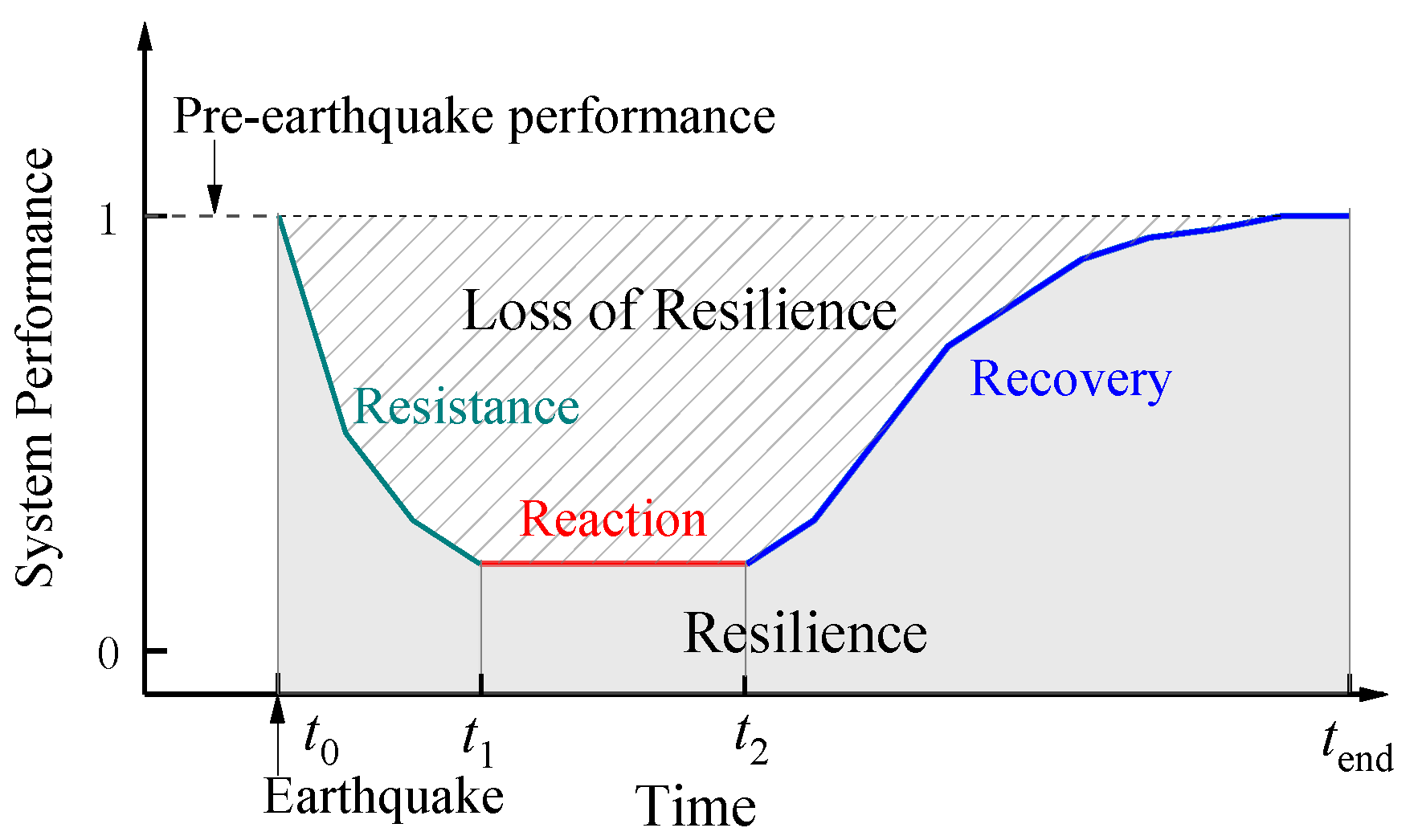
2.1. Definition of the Seismic Resilience of WDS
2.2. General Framework for Seismic Resilience Evaluation
2.3. Determine the Restoration Priority of Pipeline Damages
2.3.1. Introduction to Existing Methods
2.3.2. The Dynamic Cost-benefit Method
- Calculate F(S) by Equation (2), and the performance of the WDS is in the current status S.
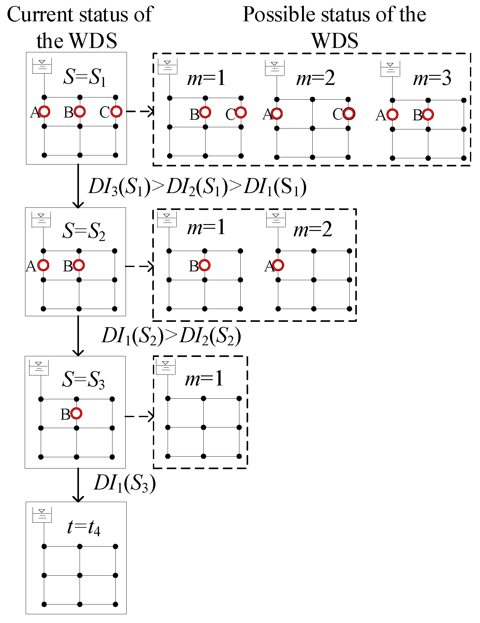
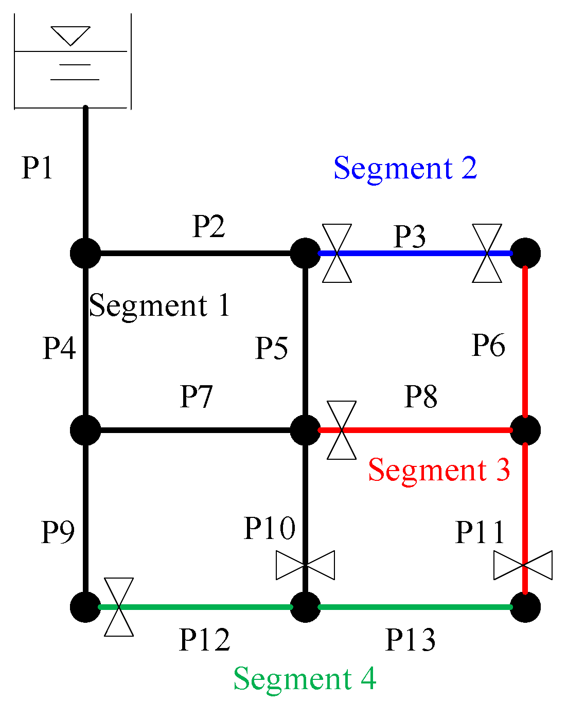
- Obtain the actions set and the time taken by each action in the current status S. For instance, the actions set is {1, 2, 3} in the status S1, while {1, 2} in the status S2 (see Figure 3).
- Calculate the performance of the WDS in the status S while the action m is completed, F (S+m). Evaluate the performance growth of the WDS, ΔFm(S) = F (S+m)-F(S).
- Evaluate the DIm(S) for each action m according to Equation (6).
- Give higher priority to the action with higher DIm(S), and update the current status once the action has been performed.
- Repeat 1~5 until all the restoration actions are performed.
- Each restoration action gets a dynamic importance indicator.
2.4. Post-Earthquake Restoration Simulation
2.4.1. Assumptions and Simplifications
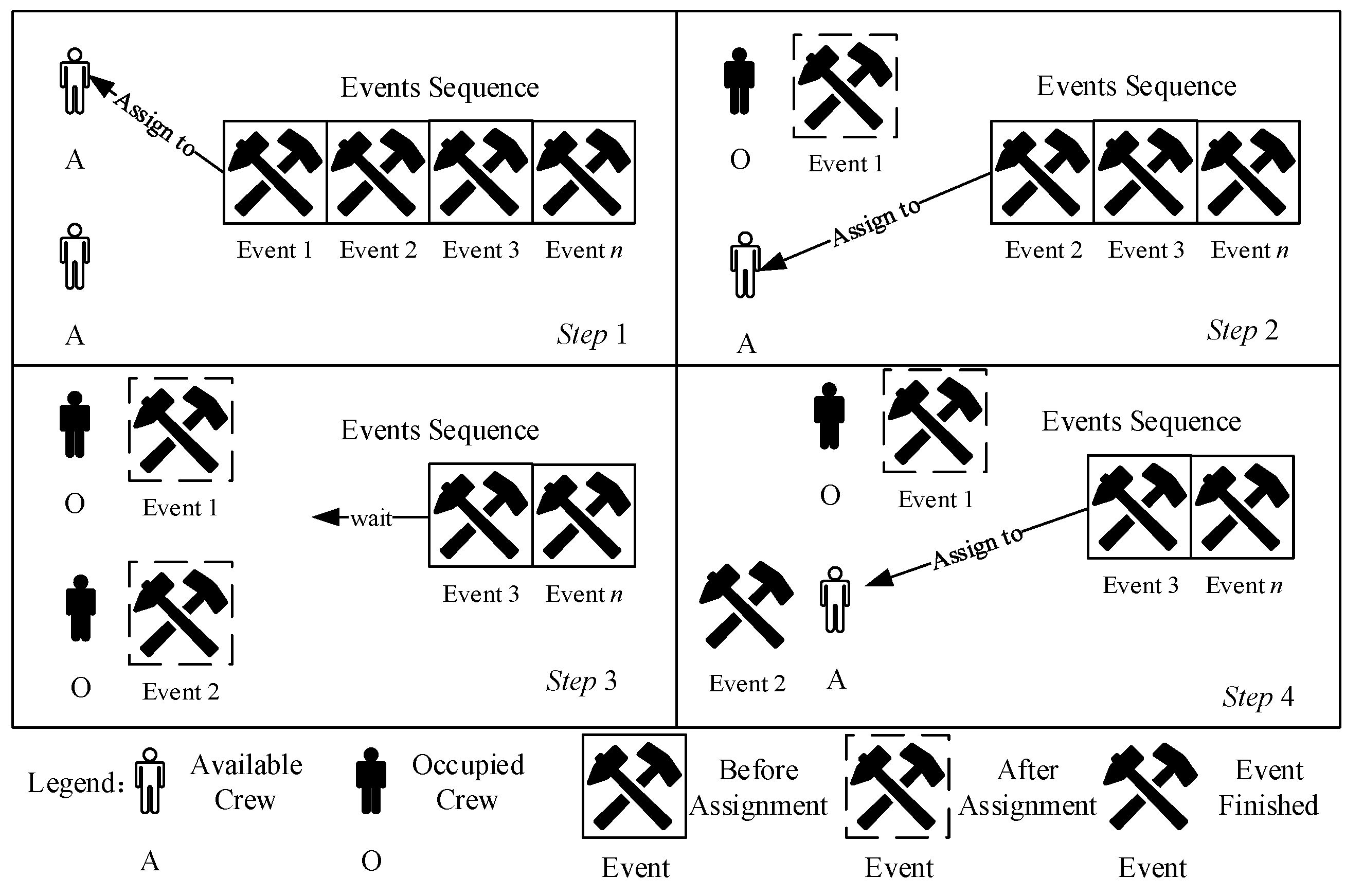
2.4.2. The Simulation Model of the Restoration Process
2.4.3. Performance Assessment of the WDS
3. Application and Results
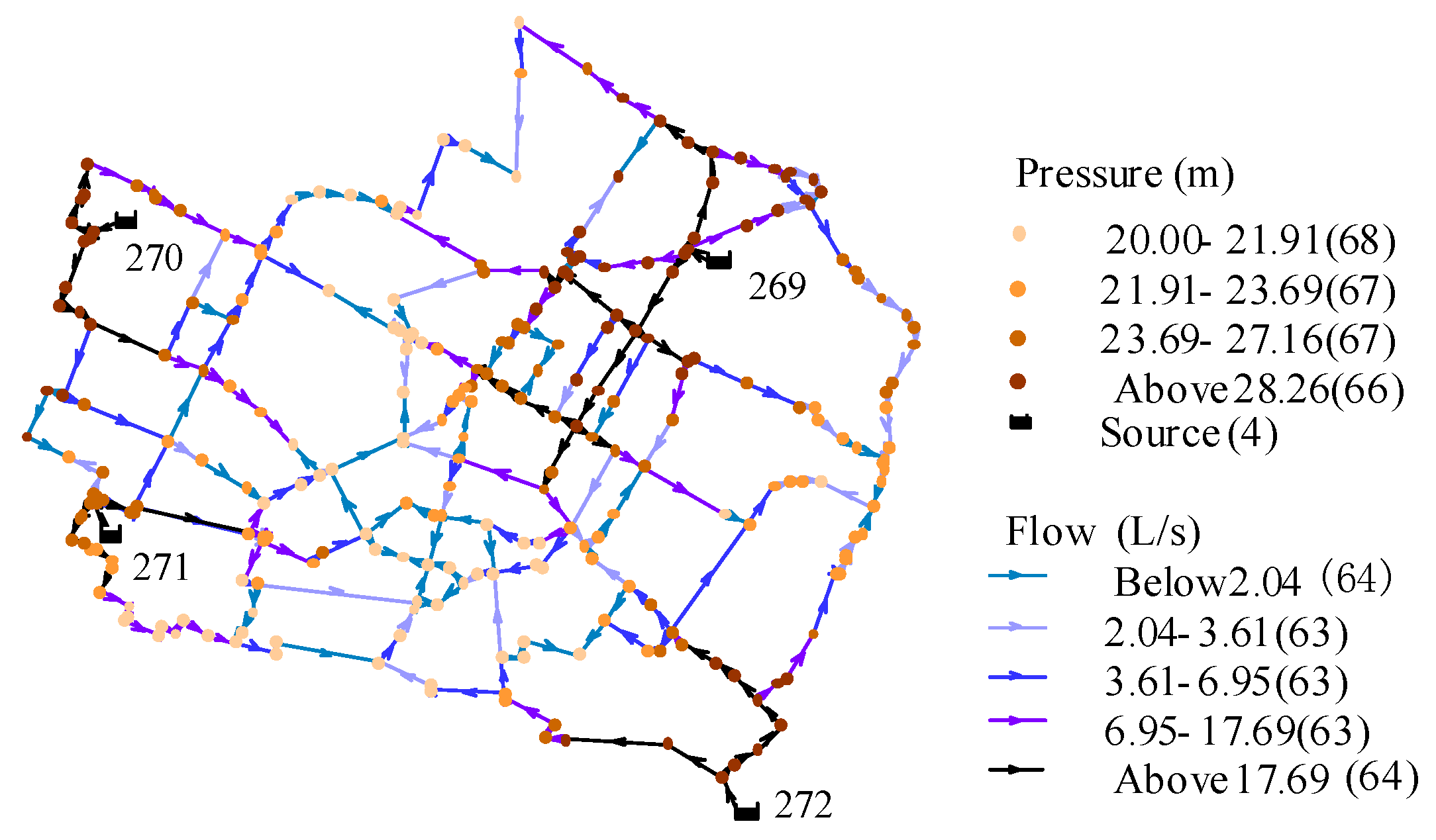
3.1. Example Network and Damage Scenarios
3.2. Parameters of the Restoration Simulation
3.3. Results of Applications (Valves at Both Ends of Pipelines)
3.3.1. Comparison of Resilience Index (RI)
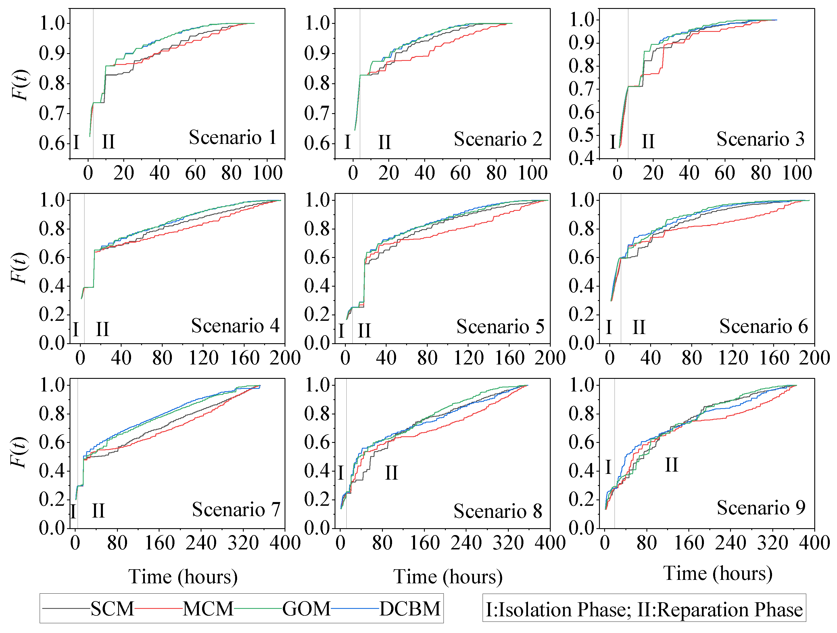
3.3.2. Overview of Performance Curves
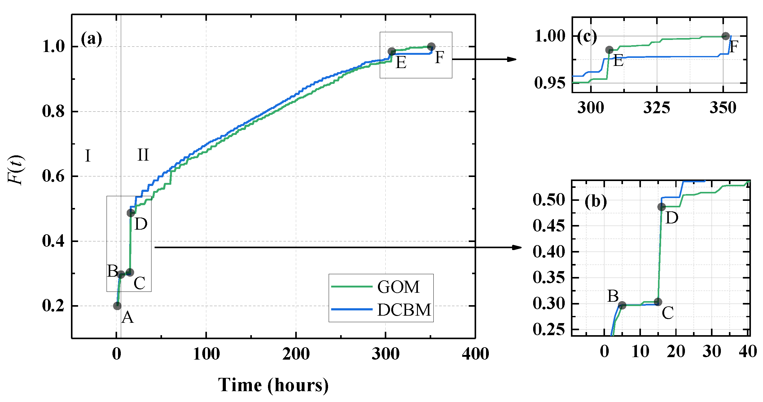
3.3.3. Performance Curves of GOM and DCBM in Scenario 7
3.3.4. Performance Curves of SCM, MCM, and DCBM in Scenario 6
3.3.5. Computation Complexity of the Four Methods
3.4. Results of Application (Considering Positions of Valves)
4. Conclusions
Supplementary Materials
Author Contributions
Funding
Acknowledgments
Conflicts of Interest
References
- Takada, S.; Tanabe, K. Three-Dimensional Seismic Response Analysis of Buried Continuous or Jointed Pipelines. J. Press. Vessel. Technol. 1987, 109, 80–87. [Google Scholar] [CrossRef]
- O’Rourke, M.J.; Liu, X. Response of Buried Pipelines Subject to Earthquake Effects; Monograph series/Multidisciplinary Cernter for Earthquake Engineering Research; Multidisciplinary Center for Earthquake Engineering Research: Buffalo, NY, USA, 1999; ISBN 0-9656682-3-1. [Google Scholar]
- Shi, P. Seismic wave propagation effects on buried segmented pipelines. Soil Dyn. Earthq. Eng. 2015, 72, 89–98. [Google Scholar] [CrossRef]
- Isoyama, R.; Ishida, E.; Yune, K.; Shirozu, T. Seismic damage estimation procedure for water supply pipelines. In Proceedings of the 12th World Conference on Earthquake Engineering, Auckland, New Zealang, 30 January–4 February 2000; Volume 18, pp. 63–68. [Google Scholar]
- Jeon, S.-S.; O’Rourke, T.D. Northridge Earthquake Effects on Pipelines and Residential Buildings. Bull. Seism. Soc. Am. 2005, 95, 294–318. [Google Scholar] [CrossRef]
- American Lifelines Alliance. Seismic Fragility Formulations for Water Systems Part I; G&E Engineering Systems Inc.: Oakland, CA, USA, 2001. [Google Scholar]
- Li, J.; He, J. A recursive decomposition algorithm for network seismic reliability evaluation. Earthq. Eng. Struct. Dyn. 2002, 31, 1525–1539. [Google Scholar] [CrossRef]
- Adachi, T.; Ellingwood, B.R. Serviceability of earthquake-damaged water systems: Effects of electrical power availability and power backup systems on system vulnerability. Reliab. Eng. Syst. Saf. 2008, 93, 78–88. [Google Scholar] [CrossRef]
- Lim, H.-W.; Song, J. Efficient risk assessment of lifeline networks under spatially correlated ground motions using selective recursive decomposition algorithm. Earthq. Eng. Struct. Dyn. 2012, 41, 1861–1882. [Google Scholar] [CrossRef]
- Hwang, H.H.M.; Lin, H.; Shinozuka, M. Seismic Performance Assessment of Water Delivery Systems. J. Infrastruct. Syst. 1998, 4, 118–125. [Google Scholar] [CrossRef]
- Shi, P.X.; O’Rourke, T.D. Seismic Response Modeling of Water Supply Systems; School of Civil & Environmental Engineering, Cornell University: Ithaca, NY, USA, 2008. [Google Scholar]
- Yoo, D.G.; Jung, D.; Kang, D.; Kim, J.H. Seismic Reliability–Based Multiobjective Design of Water Distribution System: Sensitivity Analysis. J. Water Resour. Plan. Manag. 2017, 143, 06016005. [Google Scholar] [CrossRef]
- Laucelli, D.B.; Giustolisi, O. Vulnerability Assessment of Water Distribution Networks under Seismic Actions. J. Water Resour. Plan. Manag. 2015, 141, 04014082. [Google Scholar] [CrossRef]
- Bruneau, M.; Chang, S.E.; Eguchi, R.T.; Lee, G.C.; O’Rourke, T.D.; Reinhorn, A.M.; Shinozuka, M.; Tierney, K.; Wallace, W.A.; Von Winterfeldt, D. A Framework to Quantitatively Assess and Enhance the Seismic Resilience of Communities. Earthq. Spectra 2003, 19, 733–752. [Google Scholar] [CrossRef] [Green Version]
- Davis, C.A. Water System Service Categories, Post-Earthquake Interaction, and Restoration Strategies. Earthq. Spectra 2014, 30, 1487–1509. [Google Scholar] [CrossRef]
- Cimellaro, G.P.; Tinebra, A.; Renschler, C.S.; Fragiadakis, M. New Resilience Index for Urban Water Distribution Networks. J. Struct. Eng. 2016, 142, 4015014. [Google Scholar] [CrossRef]
- Diao, K.; Sweetapple, C.; Farmani, R.; Fu, G.; Ward, S.; Butler, D. Global resilience analysis of water distribution systems. Water Res. 2016, 106, 383–393. [Google Scholar] [CrossRef] [PubMed] [Green Version]
- Shi, P.X.; O’Rourke, T.D.; Wang, Y. Simulation of earthquake water supply performance. In Proceedings of the 8th National Conference on Earthquake Engineering, Oakland, CA, USA, 18–22 April 2006. [Google Scholar]
- Davis, C.A.; O’Rourke, T.D.; Adams, M.L.; Rho, M.A. Case study: Los Angeles water services restoration following the 1994 Northridge earthquake. In Proceedings of the 15th World Conference on Earthquake Engineering (15WCEE), Lisbon, Portugal, 24–28 September 2012. [Google Scholar]
- Giovinazzi, S.; Wilson, T.; Davis, C.; Bristow, D.; Gallagher, M.; Schofield, A.; Villemure, M.; Eidinger, J.; Tang, A. Lifelines performance and management following the 22 February 2011 Christchurch earthquake, New Zealand. Bull. New Zealand Soc. Earthq. Eng. 2011, 44, 402–417. [Google Scholar] [CrossRef] [Green Version]
- Kammouh, O.; Cimellaro, G.P.; Mahin, S.A. Downtime estimation and analysis of lifelines after an earthquake. Eng. Struct. 2018, 173, 393–403. [Google Scholar] [CrossRef]
- Choi, J.; Yoo, D.G.; Kang, D. Post-earthquake restoration simulation model for water supply networks. Sustainability 2018, 10, 3618. [Google Scholar] [CrossRef] [Green Version]
- Balut, A.; Brodziak, R.; Bylka, J.; Zakrzewski, P. Battle of post-disaster response and restauration (BPDRR). In Proceedings of the 1st International Water Distribution System Analysis/Computing and Control in the Water Industry Joint Conference, Kingston, ON, Canada, 23–25 July 2018. [Google Scholar]
- Deuerlein, J.; Gilbert, D.; Abraham, E.; Piller, O. A greedy scheduling of post-disaster response and restoration using pressure-driven models and graph segment analysis. In Proceedings of the 1st International Water Distribution System Analysis/Computing and Control in the Water Industry Joint Conference, Kingston, ON, Canada, 23–25 July 2018. [Google Scholar]
- Castro-Gama, M.E.; Quintiliani, C.; Santopietro, S. After earthquake post-disaster response using a many-objective approach, a greedy and engineering Interventions. In Proceedings of the 1st International Water Distribution System Analysis/Computing and Control in the Water Industry Joint Conference, Kingston, ON, Canada, 23–25 July 2018. [Google Scholar]
- Zhang, Q.; Zheng, F.; Diao, K.; Ulanicki, B.; Huang, Y. Solving the battle of post-disaster response and restauration (BPDRR) problem with the aid of multi-phase optimization framework. In Proceedings of the 1st International Water Distribution System Analysis/Computing and Control in the Water Industry Joint Conference, Kingston, ON, Canada, 23–25 July 2018. [Google Scholar]
- Li, Y.; Gao, J.; Jian, C.; Ou, C.; Hu, S. A two-stage post-disaster response and restoration method for the water distribution system. In Proceedings of the 1st International Water Distribution System Analysis/Computing and Control in the Water Industry Joint Conference, Kingston, ON, Canada, 23–25 July 2018. [Google Scholar]
- Morley, M.S.; Tricarico, C. Pressure Driven Demand Extension for EPANET (EPANETpdd); Centre for Water Systems, University of Exeter: Exeter, UK, 2008. [Google Scholar]
- Liu, W.; Xu, L.; Li, J. Algorithms for seismic topology optimization of water distribution network. Sci. China Technol. Sci. 2012, 55, 3047–3056. [Google Scholar] [CrossRef]
- Luna, R.; Balakrishnan, N.; Dagli, C.H. Postearthquake recovery of a water distribution system: discrete event simulation using colored petri nets. J. Infrastruct. Syst. 2010, 17, 25–34. [Google Scholar] [CrossRef]
- Tabucchi, T.H.; Davidson, R.A. Post-earthquake Restoration of the Los Angeles Water Supply System; University at Buffalo: Buffalo, NY, USA, 2008. [Google Scholar]
- Ouyang, M.; Wang, Z. Resilience assessment of interdependent infrastructure systems: With a focus on joint restoration modeling and analysis. Reliab. Eng. Syst. Saf. 2015, 141, 74–82. [Google Scholar] [CrossRef]
- Sophocleous, S.; Nikoloudi, E.; Mahmoud, H.; Woodward, K.; Romano, M. Simulation-based framework for the restoration of earthquake-damaged water distribution networks using a genetic algorithm. In Proceedings of the 1st International Water Distribution System Analysis/Computing and Control in the Water Industry Joint Conference, Kingston, ON, Canada, 23–25 July 2018. [Google Scholar]
- Ouyang, M.; Dueñas-Osorio, L.; Min, X. A three-stage resilience analysis framework for urban infrastructure systems. Struct. Saf. 2012, 36–37, 23–31. [Google Scholar] [CrossRef]
- Yang, I.-C.; Peng, A.-C.; Hsu, C.-C.; Chen, K.-T. Can the emergency department sustain the first strike? Experience from the 2016 earthquake in Tainan. Hong Kong J. Emerg. Med. 2019. [Google Scholar]
- Paez, D.; Fillion, Y.; Hulley, M. Battle of post-disaster response and restauration (BPDRR): problem description and rules. In Proceedings of the 1st International Water Distribution System Analysis/Computing and Control in the Water Industry Joint Conference, Kingston, ON, Canada, 23–25 July 2018. [Google Scholar]
- Han, Z.; Ma, D.; Hou, B.; Wang, W. Post-earthquake hydraulic analyses of urban water supply network based on pressure drive demand model. Sci. Sin. Technol. 2019, 49, 351–362. [Google Scholar] [CrossRef]
- Wagner, J.M.; Shamir, U.; Marks, D.H. Water distribution reliability: simulation methods. J. Water Resour. Plan. Manag. 1988, 114, 276–294. [Google Scholar] [CrossRef] [Green Version]
- Bragalli, C.; D’Ambrosio, C.; Lee, J.; Lodi, A.; Toth, P. On the optimal design of water distribution networks: a practical MINLP approach. Optim. Eng. 2012, 13, 219–246. [Google Scholar] [CrossRef]
- Castelli, V.; Bernardini, F.; Camassi, R.; Caracciolo, C.H.; Ercolani, E.; Postpischl, L. Looking for missing earthquake traces in the Ferrara-Modena plain: an update on historical seismicity. Ann. Geophys. 2012, 55. [Google Scholar]
- Baggio, S.; Berto, L.; Rocca, I.; Saetta, A. Vulnerability assessment and seismic mitigation intervention for artistic assets: from theory to practice. Eng. Struct. 2018, 167, 272–286. [Google Scholar] [CrossRef]
- Liu, S.; Zhang, X. Investigation Report on Earthquake Disaster and Relief of Water Supply System Based on Wenchuan Earthquake; Tongji University Press: Shanghai, China, 2013; ISBN 978-7-5608-5060-3. [Google Scholar]


| No | Assumptions | Tabucchi & Davidson [31] | Luna et al. [30] | Ouyang & Wang. [34] | Zhang et al. [26] | Choi et al. [22] |
|---|---|---|---|---|---|---|
| 1 | Restoration work is independent of each other, and there is no mutual support between repair crews; | ○ | ○ | ○ | ○ | ○ |
| 2 | Regardless of the movement time of repair crews between different locations; | × | ○ | ○ | ○ | × |
| 3 | The damage locations of pipelines are determined before the restoration; | × | ○ | ○ | × | ○ |
| 4 | The repair priority of damages is determined before the restoration and keep unchanged during the restoration process; | × | ○ | ○ | × | ○ |
| 5 | Only the damages of pipeline are included, the pump stations and the tanks are intact; | ○ | ○ | × | ○ | ○ |
| 6 | The physical status of WDS changes when restoration action performed; | ○ | ○ | ○ | ○ | ○ |
| 7 | Each crew can only carry out a single restoration action at a time; | ○ | ○ | ○ | ○ | ○ |
| 8 | When a repair crew completes a task, a new repair task is assigned immediately, without rest. | × | ○ | ○ | ○ | ○ |
| Time | Events Occurred | Events Finished | The Pipe Status |
|---|---|---|---|
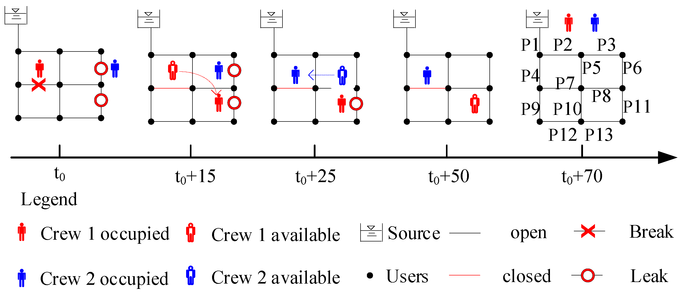
| t0 | The isolation of P7. The reparation of P6 | ----- | ----- |
| t0 + 15 | The reparation of P11 | The isolation of P7. | P7: break→closed |
| t0 + 25 | The replacement of P7 | The reparation of P6 | P6: leak→open |
| t0 + 50 | ------ | The reparation of P11 | P11: leak→open |
| t0 + 70 | ------ | The replacement of P7 | P7: closed→open |
| Damage Scenarios No. | Number of Breaks | Number of Leaks | Number of Damages |
|---|---|---|---|
| 1 | 4 | 28 | 32 |
| 2 | 10 | 22 | 32 |
| 3 | 16 | 16 | 32 |
| 4 | 8 | 64 | 72 |
| 5 | 22 | 50 | 72 |
| 6 | 36 | 36 | 72 |
| 7 | 14 | 123 | 137 |
| 8 | 42 | 95 | 137 |
| 9 | 69 | 68 | 137 |
| Abb. | Method | Description |
|---|---|---|
| SCM | the single-criterion method | Sorting the events by the hydraulic importance (HI) |
| MCM | the multi-criteria method | Primary criterion: damage type, break prior to the leak Secondary criterion: the straight-line distance to water resources |
| GOM | the global optimization method | Solved by Genetic Algorithm, the population size is 300, the evolutionary generation is 100, the crossover probability is 0.9, the mutation probability is 0.1 |
| DCBM | the dynamic cost-benefit method | Sorting the events by the DI |
| Scenario No. | SCM | MCM | GOM | DCBM |
|---|---|---|---|---|
| 1 | 0.9011 | 0.9028 | 0.9335 | 0.9335 |
| 2 | 0.9280 | 0.9071 | 0.9422 | 0.9411 |
| 3 | 0.8992 | 0.8841 | 0.9171 | 0.9146 |
| 4 | 0.8096 | 0.7846 | 0.8383 | 0.8354 |
| 5 | 0.7866 | 0.7542 | 0.8194 | 0.8200 |
| 6 | 0.8475 | 0.8098 | 0.8808 | 0.8752 |
| 7 | 0.7162 | 0.6990 | 0.7717 | 0.7853 |
| 8 | 0.7231 | 0.6886 | 0.7586 | 0.7415 |
| 9 | 0.7356 | 0.7006 | 0.7421 | 0.7446 |
| Time (hour) | GOM | DCBM | Remark | ||
|---|---|---|---|---|---|
| Event Finished | F(t) | Event Finished | F(t) | ||
| 4 | All break pips are isolated | 0.2966 | All break pips were isolated | 0.2976 | B |
| 10 | Repaired pipe 103 | 0.3033 | No action | 0.2976 | |
| 11 | No action | 0.3033 | Replaced pipe 313 | 0.2983 | C |
| 15 | Replaced pipe 292 | 0.4865 | Replaced pipe 292 | 0.5060 | D |
| 21 | Replaced pipe 59; Repaired pipe 107 | 0.5095 | Replaced pipe 59; Repaired pipe 158 | 0.5367 | |
| … | … | … | … | … | … |
| 306 | Replaced pipe 40; Repaired pipe 47 | 0.9852 | No action | 0.9759 | E |
| … | … | … | … | … | … |
| Time (hour) | Event Finished | F(t) | Remark |
|---|---|---|---|
| 10 | All break pipes are isolated | 0.5949 | B |
| 17 | Repaired pipe 66 | 0.5997 | --- |
| 20 | Repaired pipe 291 | 0.6057 | --- |
| 24 | Repaired pipe 68 | 0.6104 | C |
| 27 | Replaced pipe 135 | 0.6668 | D |
| Scenario No. | SCM | MCM | GOM | DCBM | ||||
|---|---|---|---|---|---|---|---|---|
| Number | Time(s) | Number | Time(s) | Number | Time(s) | Number | Time(s) | |
| 1 | 317 | 2.25 | 0 | 0.15 | 590626 | 3975.40 | 631 | 8.31 |
| 2 | 317 | 2.31 | 0 | 0.15 | 655128 | 4496.94 | 671 | 9.14 |
| 3 | 317 | 2.32 | 0 | 0.15 | 671438 | 7989.63 | 751 | 10.60 |
| 4 | 317 | 2.29 | 0 | 0.19 | 2445231 | 16900.74 | 2858 | 43.49 |
| 5 | 317 | 2.32 | 0 | 0.19 | 2660022 | 23482.23 | 3677 | 49.75 |
| 6 | 317 | 2.32 | 0 | 0.20 | 2269009 | 145421.06 | 3585 | 55.80 |
| 7 | 317 | 2.31 | 0 | 0.23 | 5144953 | 52331.85 | 9912 | 179.72 |
| 8 | 317 | 2.34 | 0 | 0.26 | 4562696 | 355996.76 | 10712 | 200.64 |
| 9 | 317 | 2.41 | 0 | 0.29 | 4265958 | 363976.64 | 12234 | 243.88 |
| Scenario No. | SCM | MCM | GOM | DCBM |
|---|---|---|---|---|
| 1 | 0.8587 | 0.8939 | 0.9268 | 0.9240 |
| 2 | 0.8893 | 0.9020 | 0.9410 | 0.9385 |
| 3 | 0.8651 | 0.8679 | 0.9083 | 0.9035 |
© 2020 by the authors. Licensee MDPI, Basel, Switzerland. This article is an open access article distributed under the terms and conditions of the Creative Commons Attribution (CC BY) license (http://creativecommons.org/licenses/by/4.0/).
Share and Cite
Han, Z.; Ma, D.; Hou, B.; Wang, W. Seismic Resilience Enhancement of Urban Water Distribution System Using Restoration Priority of Pipeline Damages. Sustainability 2020, 12, 914. https://doi.org/10.3390/su12030914
Han Z, Ma D, Hou B, Wang W. Seismic Resilience Enhancement of Urban Water Distribution System Using Restoration Priority of Pipeline Damages. Sustainability. 2020; 12(3):914. https://doi.org/10.3390/su12030914
Chicago/Turabian StyleHan, Zhao, Donghui Ma, Benwei Hou, and Wei Wang. 2020. "Seismic Resilience Enhancement of Urban Water Distribution System Using Restoration Priority of Pipeline Damages" Sustainability 12, no. 3: 914. https://doi.org/10.3390/su12030914