The Determinants of Carbon Emissions in the Chinese Construction Industry: A Spatial Analysis

Abstract

As the largest carbon emitter in the world, China is confronted with great challenges of mitigating carbon emissions, especially from its construction industry. Yet, the understanding of carbon emissions in the construction industry remains limited. As one of the first few attempts, this paper contributes to the literature by identifying the determinants of carbon emissions in the Chinese construction industry from the perspective of spatial spillover effects. A panel dataset of 30 provinces or municipalities from 2005 to 2015 was used for the analysis. We found that there is a significant and positive spatial autocorrelation of carbon emissions. The local Moran’s I showed local agglomeration characteristics of H-H (high-high) and L-L (low-low). The indicators of population density, economic growth, energy structure, and industrial structure had either direct or indirect effects on carbon emissions. In particular, we found that low-carbon technology innovation significantly reduces carbon emissions, both in local and neighboring regions. We also found that the industry agglomeration significantly increases carbon emissions in the local regions. Our results imply that the Chinese government can reduce carbon emissions by encouraging low-carbon technology innovations. Meanwhile, our results also highlight the negative environmental impacts of the current policies to promote industry agglomeration.

1. Introduction

Global warming caused by greenhouse gases is a global environmental issue, and has become a huge threat to the survival of human beings and other species. Among many greenhouse gases, carbon dioxide (CO₂) accounts for the largest proportion of greenhouse gases [1]. To control the global temperature, reduction in carbon emissions must be ensured in the nations of the world. With rapid urbanization and fast economic growth since the reform and opening-up policy, China has become the world’s largest emitter of greenhouse gases [2]. It is estimated that the amount of carbon emissions in China will continue to increase in the future [3]. Under this background, “low-carbon” production is viewed as the key to sustainable urban development and an effective approach to tackling climate change [4]. The control of carbon emissions has become a critical way to achieve green development.

Among many industries, the construction industry has been recognized as a major source of carbon emissions [5]. Previous research indicated that the construction industry consumes more than 40% of global energy and accounts for 36% of carbon emissions [6]. The CO₂ emissions from the construction sector in China have increased from 3905 × 104 t in 1995 to 103,721 × 104 t in 2010, accounting for 27.87% and 34.31% of China’s total carbon emissions from energy consumption, respectively [7]. It is estimated that the number is likely to increase to 35% by 2030 [8]. While China is facing huge pressure to reduce carbon emissions [9], the construction industry may have a great potential for carbon emission reduction [10]. Identifying the determinants of carbon emissions in the construction industry therefore seems critical, and may contribute to policy design to develop a low-carbon economy in China.

Some studies have investigated the determinants of carbon emissions, though they often assume that the influencing process is a static and closed system, and the determinants only affect the local regions [3,11,12]. In this paper, we propose that there may be a significant interaction of carbon emissions between neighboring regions. Indeed, some scientists have argued that the determinants of carbon emissions, such as social and economic factors or public policies, not only have a direct effect on carbon emissions in the local region, but also have an indirect effect on carbon emissions in neighboring regions, namely the spatial spillover effect [13,14]. Therefore, in this paper we identify the determinants of carbon emissions, taking into account the spatial spillover effects. To the best of our knowledge, this paper is one of the first few attempts to analyze the determinants of carbon emissions in the construction industry from the perspective of the spatial spillover effect.

The rest of the paper is structured as follows: first, we review the relevant literature on the determinants of carbon emissions (Section 2); second, we introduce the data and method used in the paper (Section 3); third, we report the results of data analysis (Section 4); fourth, we discuss the research results (Section 5); finally, we conclude the major findings (Section 6).

2. Literature Review

Identifying the determinants of carbon emissions is the premise to realizing the carbon emission reduction target [11,15]. The major methods to identify the determinants of carbon emissions in the construction industry are the index decomposition analysis (IDA) and the structural decomposition analysis (SDA). The IDA has a wider application than the SDA for its flexibility and lower data requirement [10,16,17,18]. However, the IDA only focuses on the direct effect and ignores the effect of the indirect energy demand and final demand [1,19,20]. Compared to IDA, the SDA analyzes carbon emissions through the input–output model framework, allowing for the detection of both the direct and indirect carbon emissions of energy consumption. The SDA also distinguishes between a range of technological and structural effects. For example, Shi et al. [1] investigated the determinants of carbon emissions in the Chinese construction industry using the SDA, and found that the total final demand effect contributed the most to the increase in carbon emissions, while energy intensity effect offset the largest part of the increase. However, the application of SDA in China may be inappropriate because the Chinese database of input–output is not updated yearly. Such data intermittency may lead to inaccurate results [21].

Previous studies paid little attention to the spatial spillover effects when examining the determinants of carbon emissions in the construction industry [1,16,17,18]. They assumed that the studied regions were spatially independent from each other, and the characteristics of one region would not affect the carbon emissions of its neighboring regions. However, some research found that space factors had important impacts on natural and social phenomenon [22]. In particular, Li et al. [23] depicted the temporal and spatial heterogeneity of carbon intensity in China’s construction industry, and found spatial cluster effects in neighboring provinces. Regional characteristics, e.g., population, economic growth, and technology innovation, may affect not only the local carbon emissions, but also the carbon emissions in neighboring regions. A growing number of studies have employed spatial econometrics to detect spatial autocorrelation when analyzing the determinants of carbon emissions [24,25,26,27], which may serve as references for the spatial spillover effect of carbon emissions in the construction industry.

To measure the spatial spillover effects, a spatial weight matrix can be incorporated into the Stochastic Impacts by Regression on Population, Affluence, and Technology (STIRPAT) model. With different assumptions, three types of spatial econometrics models, spatial autoregressive model (SAR), spatial error model (SEM), and spatial Durbin model (SDM), are often employed in empirical work [22]. While the SAR model assumes that economic variables in a given region affect other regions through a spatial transmission mechanism, the SEM model concentrates on the regional spillover effect by random shocks and the relevance of the interregional degree of correlation embodied in error terms [26]. The SDM model is the general form of the SAR and SEM models and takes into account both endogenous and exogenous spatial interaction effects [28].

3. Methodology

3.1. Measuring Carbon Emissions

Measuring carbon emissions for the construction industry is different from those for a single building, which usually predicts carbon emissions based on on-site survey data of detailed energy and material consumption of the building [29]. Several methods are available to measure carbon emissions in the construction industry, e.g., the carbon emission coefficient method, based on the terminal energy consumption [23], and the input–output method [1,30,31]. Due to data availability, we adopted the carbon emission coefficient method recommended by the Intergovernmental Panel on Climate Change (IPCC) report to calculate carbon emissions in the construction industry. We considered both direct carbon emissions due to energy consumption in the construction industry and indirect carbon emissions generated by the production of building materials, because indirect carbon emissions could be considerably large.

In this paper, the construction industry refers to the material production department engaged in survey, design, construction, and maintenance activities of the original building in the national economy. The total carbon emissions in the construction industry for each province consist of direct and indirect carbon emissions, and are calculated following Equation (1):

$$C=C_{dir}+C_{indir},$$

(1)

where $C$ is the total carbon emissions, $C_{dir}$ is the direct carbon emissions. Typically, there are different scopes to calculate the direct carbon emissions [32]. In line with the scope used by Li et al. [23], we calculated the direct carbon emissions in the construction industry only from the consumption side. In other words, energies used for generating other forms of energy, e.g., electricity, were not part of our calculation. Such a choice raises a fair assumption that the task to reduce carbon emissions belongs to the consumption regions instead of the production regions. Specifically, we considered 11 types of energy, according to the actual terminal energy consumption requirements of the construction industry. Following the IPCC guidelines for National Greenhouse Gas Inventories in 2006, we used Equation (2) to measure the direct emissions:

$$C_{dir}=\frac{12}{44}\times {{\displaystyle \sum }}_{k=1}^{11}{E}_k\times {\alpha }_k\times {\beta }_k,$$

(2)

where 44 and 12 are the molecular weights of carbon dioxide and carbon, respectively; $k$ is the energy type shown in Table 1 ($k$ = 1,2,…,11) (we selected 11 types of energy that are primarily used in China’s construction industry. In 2005, the 11 energies accounted for 99.81% of the total energy consumption in China’s construction industry. The shares of each energy are: raw coal (21.49%), other washed coal (0.10%), coke (1.12%), gasoline (12.45%), diesel (25.89%), fuel oil (0.83%), liquefied petroleum gas (0.44%), other oil (24.07%), natural gas (0.81%), heat (1.19%), and electricity (11.41%)); $E_k$ is the terminal consumption of the kth energy in the construction industry; ${\alpha }_k$ is the standard coal coefficient of the kth energy; ${\beta }_k$ is the carbon emission coefficient of the kth energy.

Table 1. The carbon emissions coefficients of energies.

Energy	Standard Coal Coefficient	CO2 Emissions Factor
Raw coal	0.7143 kg ce/kg	0.7669 kg CO2/kg ce
Other washed Coal	0.45 kg ce/kg	0.8079 kg CO2/kg ce
Coke	0.9714 kg ce/kg	0.8547 kg CO2/kg ce
Gasoline	1.4714 kg ce/kg	0.5571 kg CO2/kg ce
Diesel	1.4571 kg ce/kg	0.5913 kg CO2/kg ce
Fuel oil	1.4286 kg ce/kg	0.6176 kg CO2/kg ce
Liquefied petroleum gas	1.7143 kg ce/kg	0.5035 kg CO2/kg ce
Other oil	1.20 kg ce/kg	0.5854 kg CO2/kg ce
Natural gas	1.33 kg ce/m3	0.4478 kg CO2/kg ce
Heat	0.034 kg ce/106 J	0.8948 kg CO2/kg ce
Electricity	0.1229 kg ce/kwh	0.277 kg CO2/kg ce

Source: China Energy Statistical Yearbooks.

$C_{indir}$ is the indirect carbon emissions, which resulted from the industries consuming building materials [33], such as steel, wood, cement, glass, and aluminum. The consumption of building materials was obtained from the China Statistical Yearbooks on Construction. Because some building materials can be recycled, we took the recyclability into account in the calculation process. The carbon emissions of building materials were calculated following Equation (3):

$$C_{indir}=\frac{12}{44}\times {{\displaystyle \sum }}_{m=1}^5{M}_m\times {\gamma }_m\times \left(1-{\epsilon }_m\right),$$

(3)

where $M_m$ is the consumption of the mth building material; ${\gamma }_m$ is the carbon emission coefficient of the mth building material; ${\epsilon }_m$ is the recoverability rate of the mth building material. Table 2 shows the carbon emission coefficients and recoverability rates of the five different building materials.

Table 2. The carbon emissions and recovery coefficients of building materials.

Building Materials	Steel	Wood	Cement	Glass	Aluminum
CO2 emissions coefficient	1.789 kg/kg	−0.8423 t/m3	1.277 kg/kg	0.02728 t/heavy box	2.6 kg/kg
Recovery coefficient	0.8	0.1	-	0.13	0.85

Sources: The CO₂ emission coefficients of building materials are from the existing research [34,35,36]. The recoverability rates of building materials are from the existing research [37,38]. Since wood absorbs CO₂ in the production process, its CO₂ emissions coefficient is negative.

3.2. Spatial Autocorrelation Index

We used Moran’s index, which reflects the similarity of carbon emissions between regions, to measure spatial autocorrelation [39]. Both the global and local Moran’s index were estimated. Global Moran’s I reflects the degree of spatial auto-dependency of variables over the entire region. The value of global Moran’s I ranges from −1 to 1. If the value is >0, it means positive autocorrelation, and the greater the value, the greater the degree of spatial agglomeration; if the value is <0, it means negative autocorrelation, and the smaller the value, the greater the difference; if the value is close to 0, there is no spatial autocorrelation. The calculation is shown in Equation (4):

$$Mora{n}^{\prime }s I=\frac{n}{{{\displaystyle \sum }}_{i=1}^n{\left(c_i-\overline{c}\right)}^2}\times \frac{{{\displaystyle \sum }}_{i=1}^n{{\displaystyle \sum }}_{j=1}^n{W}_{ij}\left(c_i-\overline{c}\right)\left(c_j-\overline{c}\right)}{{{\displaystyle \sum }}_{i=1}^n{{\displaystyle \sum }}_{j=1}^n{W}_{ij}},$$

(4)

where $n$ represents the number of provinces in China; $c_i$ and $c_j$ represent carbon emissions in province $i$ and $j$, respectively; $\overline{c}$ is the average carbon emissions in all provinces; $W_{ij}$ is the spatial weight matrix, and represents the spatial disparity between region $i$ and $j$ [40].

The spatial weight matrix is a key to analyze spatial autocorrelation among regions. In this study, we constructed two spatial weight matrixes. The first one was the contiguity spatial weight matrix. We applied the default but most commonly used contiguity matrix, namely queen contiguity, which treats regions that share a common border or a single common point as neighbors [41]. It is noted as W₁ and set as [26]:

$$W_1=\{\begin{array}{l}1, if share a common border or a single common point\\ 0,else\end{array}.$$

(5)

The second one was the economic weight matrix, which measures economic proximity among regions. Following Han [27], we used the relative difference in average GDP per capita between two regions to capture economic distance. It is noted as W₂ and set as:

$$W_2=1/\left|{\overline{PGDP}}_i-{\overline{PGDP}}_j\right|,$$

(6)

where ${\overline{PGDP}}_i$ is the average GDP per capita in region $i$ in 2005–2015, and $i\ne j$. If two regions’ economic growth is similar, the governance strategy in the regions on carbon emissions should be similar, too.

To test the significance of global Moran’s I, the Z value was calculated following Equation (7):

$$Z=\left(I-E\left(I\right)\right)/\sqrt{Var\left(I\right)} \stackrel{d}{\to } N\left(0,1\right),$$

(7)

where $E\left(I\right)$ represents the expected value of Moran’s I; $Var\left(I\right)$ refers to the variance of Moran’s I. The Z-value is tested using a threshold value of the standard normal state, i.e., if the Z value passes the significance test at the three levels of 10%, 5%, or 1%, Moran’s I is of great significance.

Local Moran’s I reflects the spatial agglomeration near region $i$. If the local spatial autocorrelation is significant, the Moran scatter chart can divide the relationship between region $i$ and its neighboring regions into four types: HH (high-high), LL (low-low), HL (high-low), and LH (low-high). HH(LL) indicates that the high(low) value of region $i$ is surrounded by the high(low) value regions, i.e., there is positive spatial autocorrelation with spatial agglomeration effect. HL(LH) indicates that the high(low) value of region $i$ is surrounded by the low(high) value regions, i.e., there is negative spatial autocorrelation. Local Moran’s I is defined in Equation (8):

$$I_i=\frac{n\left(c_i-\overline{c}\right)}{{{\displaystyle \sum }}_{i=1}^n{\left(c_i-\overline{c}\right)}^2}\times {\displaystyle \sum }_{j=1}^n{W}_{ij}\left(c_j-\overline{c}\right).$$

(8)

3.3. Spatial Panel Econometric Model

The STIRPAT model developed by Dietz and Rosa [42] is often employed to investigate the non-proportionate impacts of variables on the environment. The standard STIRPAT model is:

$$I=a{P}^{{\alpha }_1}{A}^{{\alpha }_2}{T}^{{\alpha }_3}e,$$

(9)

where $a$ represents the constant; ${\alpha }_1$, ${\alpha }_2$ and ${\alpha }_3$ are the exponential terms of population size ($P$), affluence ($A$) and technology ($T$), respectively; $e$ is the error term; $I$ is the environmental pressure.

In order to estimate the determinants of carbon emissions in the construction industry, especially the technology factor, we extended the model by applying it to the carbon emission context and adding other variables into the model, and then took the logarithmic form of the model to overcome potential heteroscedasticity. The logarithm of the model is more flexible. The extended STIRPAT model is defined as follows:

$$\ln C_{it}=a+{\alpha }_1\ln PO{P}_{it}+{\alpha }_2\ln PGD{P}_{it}+{\alpha }_3\ln PA{T}_{it}+{\alpha }_4\ln E{S}_{it}+{\alpha }_5\ln I{S}_{it}+{\alpha }_6\ln E{I}_{it}+{\alpha }_7\ln I{A}_{it}+e_{it},$$

(10)

where carbon emissions per capita (C) is the dependent variable, which is the ratio of carbon emissions obtained following Equations (1)–(3) to population size. We used urban population density (POP) in each province at the end of the year to represent P. We did not use the total population density in the region because the construction industry is mainly located in urban areas. According to the previous studies [43,44], we selected GDP per capita (PGDP) to represent A. We selected several factors to represent T. According to Dietz and Rosa [42], T is not a single factor but comprises many separate factors that influence the environment. In a few studies, T was interpreted as the residual term [45,46]. In some other studies [44,47,48], T may be represented by multiple different variables, including energy intensity, energy structure, urbanization, and industrialization. In more recent studies, the stock of technical patents associated with carbon emissions was also used to represent T [49,50,51]. Furthermore, T may also consist of industrial agglomeration, which can not only use the price and competition mechanism to improve the efficiency of energy resource allocation, but also take advantage of knowledge spillovers, technology innovation, and energy efficiency [52]. According to the data availability, we selected the applied low-carbon technology patents (PAT), energy structure (ES), industrial structure (IS), energy intensity (EI), and industrial agglomeration (IA) to represent T. The detailed definitions and descriptive statistics of these variables are shown in Table 3.

Table 3. Variables and data definitions.

Variable	Definition	Mean	Std. Dev.	Max	Min
C	carbon emissions per capita= carbon emissions/population (t/person)	0.763	0.767	6.325	0.077
POP	population density = urban population/built-up area (104 persons/km2)	1.698	0.407	2.779	0.804
PGDP	GDP per capita = GDP/total population (104 Yuan/person)	2.928	1.895	10.294	0.505
PAT	items of patent per unit output value = items of patent applications/construction industry output value (item/108 Yuan)	0.074	0.105	0.346	0.002
ES	energy structure = fossil energy (coal and oil) consumption of construction industry/total energy consumption of construction industry (%)	0.751	0.147	0.999	0.116
IS	industrial structure = the output value of building and civil engineering construction industry/total output value of construction industry (%)	0.580	0.131	0.876	0.187
EI	energy intensity = total energy consumption of construction industry/total output value of construction industry (t/104 Yuan)	0.076	0.055	0.437	0.007
IA	industry agglomeration (Following Zhao et al. [52], industry agglomeration was calculated as follows: $I{A}_{ij}=\left(q_{ij}/q_j\right)/\left(q_i/q\right)$, where $q_{ij}$ refers to the output of $i$ industry in region $j$, $q_j$ refers to the total output of region $j$, $q_i$ refers to the output of $i$ industry in the nation, $q$ refers to the total output of the nation.)	0.954	0.357	2.232	0.251

Notes: Authors’ own computation.

We adopted the SDM model to control for the spatial spillover effects when analyzing the determinants of carbon emissions. The model is as follows:

$$C_{it}=a+\delta {{\displaystyle \sum }}_{j=1}^n{W}_{ij}{C}_{it}+\beta x_{it}+{{\displaystyle \sum }}_{j=1}^n{W}_{ij}{x}_{it}\theta +{\mu }_i+v_t+{\epsilon }_{it},$$

(11)

where $C_{it}$ is the dependent variable, $x_{it}$ is the independent variable, $\beta$ is the coefficient of independent variable, $a$ is the constant, $\delta$ is spatial lag coefficients, $\theta$ is the spatial lag coefficients of independent variables, ${\mu }_i$ and $v_t$ are regional and time effects, ${\epsilon }_{it}$ is the vector of residual, $W_{ij}$ is the spatial weights matrix, $\beta x_{it}$ refers to the effect of independent variables on the dependent variable in the region $i$ at time $t$, $W_{ij}{x}_{it}$ is the effect of independent variables on carbon emissions in other regions, namely spatial spillover effects. We employed the maximum likelihood (ML) method [53] to estimate the spatial panel models.

3.4. Data

We used a panel dataset of 30 provinces or municipalities in China from 2005 to 2015 (Tibet, Taiwan, Hong Kong, and Macao were excluded due to data availability) for this analysis. Gross domestic product (GDP), total and urban population, output value of the construction industry, and the output value of the building and civil engineering construction industry of each province were collected from the China Statistical Yearbooks (data from the China Statistical Yearbooks were used to study the same topic (cf. Wu et al. [9] and Li et al. [23])). We converted the GDP and the output value of construction industry into 2005 constant price (RMB Yuan). The information about patents was obtained from the Y02B indexing scheme in the cooperative patent classification jointly issued by the United States and the United Kingdom. Here, we only considered the patents applied by the Chinese people and that applied in China.

4. Results

4.1. Spatial Distribution of Carbon Emissions

Using Equations (1)–(3), we calculated the carbon emissions in the construction industry. Figure 1 shows the distributions of carbon emission in 2005 and 2015, which employed the natural breaks method with ArcGIS to rank the carbon emissions of different regions. Compared to the carbon emissions in 2005, the carbon emissions in 2015 have grown dramatically, with the highest value increased from 4664 × 10⁴ t in 2005 to 12,644 × 10⁴ t in 2015. Figure 1 also shows that Shanghai, Jiangsu, and Zhejiang were always the largest emitters, while the other coastal regions and the middle regions in China emitted moderately. Western regions often had the lowest levels of carbon emissions. Such distribution of carbon emissions in different regions is generally consistent with the regional characteristics. For example, the level of economic growth, population density, and the added value from the construction industry are often the highest in the eastern regions (especially in Shanghai, Jiangsu, and Zhejiang, often known as the Yangtze River Delta) and the lowest in the western regions.

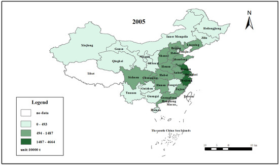
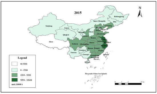
Figure 1. Carbon emissions in construction industry in 2005 and 2015.

4.2. Spatial Autocorrelation Results

Table 4 shows the global Moran’s I from 2005 to 2015. When the contiguity spatial weight matrix (W₁) was used, the global Moran’s I of carbon emissions in the construction industry mostly showed significant spatial autocorrelation, with a statistical significance level of less than 0.05. The global Moran’s I was positive, suggesting the presence of a positive spatial autocorrelation. When the economic weight matrix (W₂) was used, the p-values of global Moran’s I of carbon emissions were mostly larger than 0.10, suggesting the economic autocorrelation is insignificant. These results indicate that the global spatial autocorrelation of carbon emissions in the construction industry is more likely to occur in geographical connection. Therefore, the following spatial econometric model analyzed the spatial spillover effect based on the contiguity spatial weight matrix.

Table 4. The global Moran’s I of carbon emissions.

Time	W1			W2
	Moran’s I	Z	p	Moran’s I	Z	p
2005	0.359	3.413	0.000	0.170	1.878	0.030
2006	0.275	2.687	0.004	0.092	1.167	0.122
2007	0.300	2.918	0.002	0.061	0.885	0.188
2008	0.234	2.298	0.011	0.064	0.893	0.186
2009	0.206	2.062	0.020	0.078	1.021	0.154
2010	0.183	1.804	0.036	−0.025	0.085	0.466
2011	0.044	0.674	0.250	0.101	1.232	0.109
2012	0.052	0.729	0.233	0.094	1.151	0.125
2013	0.022	0.464	0.321	0.057	0.801	0.212
2014	−0.010	0.204	0.419	−0.175	−1.231	0.109
2015	0.249	2.409	0.008	0.110	1.304	0.096

Notes: Authors’ own computation.

We also estimated the local Moran’s I to test the local spatial autocorrelation of carbon emissions using data of 2005 and 2015. Figure 2 shows the results. We found that most regions fell into the first and the third quadrants, indicating that regions with high(low) carbon emissions are more likely to be close to regions with high(low) carbon emissions. Specifically, the regions in the first quadrant were mainly located in eastern China, such as Jiangsu, Zhejiang, Fujian, and Shanghai, and Central China, such as Hubei; the regions in the third quadrant were mainly located in western China, such as Inner Mongolia, Guangxi, Gansu, Qinghai, Ningxia, and Xinjiang, and Northeast China, such as Heilongjiang and Jilin. We did not find a significant change in the number of regions with positive spatial autocorrelation. In 2005 and 2015 the number was 23 and 25, respectively.

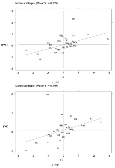
Figure 2. Local Moran’s I scatterplot. Notes: BJ—Beijing, TJ—Tianjin, HEB—Hebei, SXI—Shanxi, NM—Inner Mongolia, LN—Liaoning, JL—Jilin, HLJ—Heilongjiang, SH—Shanghai, JS—Jiangsu, ZJ—Zhejiang, AH—Anhui, FJ—Fujian, JX—Jiangxi, SD—Shandong, HEN—Henan, HUB—Hubei, HUN—Hunan, GD—Guangdong, GX—Guangxi, HN—Hainan, CQ—Chongqing, SC—Sichuan, GZ—Guizhou, YN—Yunnan, SNX—Shaanxi, GS—Gansu, QH—Qinghai, NX—Ningxia, XJ—Xinjiang. As space is limited, this study only shows the scatterplot chart in 2005 and 2015.

4.3. Choice of Spatial Econometric Models

The statistical significance of Moran’s I implies that the results from econometric models which do not take into account spatial autocorrelation will be biased [54]. In this paper, we further performed the Lagrange Multiplier (LM) tests to determine whether a spatial econometric model was preferred to non-spatial econometric model. Table 5 shows that the LM-lag, Robust LM-lag, LM-error, and Robust LM-error tests were all significant at the 1% level, indicating the necessity of selecting the spatial econometric model to analyze the determinants. Conditional on the selection of the spatial econometric model, we tested whether the SDM could be simplified to the SAR or SEM, using the Likelihood Ratio (LR) tests. The results show that the values of LR-lag and LR-error statistics were significant at the 1% level, suggesting that the SDM could not be simplified into the SAR or SEM model. Given the panel nature of our dataset, we performed the Hausman test to decide whether the fixed effect model or the random effect model should be followed. If the unobservable variables that represent individual heterogeneity are related to an explanatory variable, we call it a “fixed effect model”; if they are not related to all explanatory variables, we call it a “random effect model”. The results rejected the null hypothesis at the 1% level, supporting the selection of the fixed effect model. Based on the log-likelihood value and the economic meaning of the explanatory variables, we found that simultaneous control on both the spatial and temporal effects in SDM was better (see Table 6). According to the above tests, we adopted the spatial–temporal fixed spatial Durbin model.

Table 5. Spatial econometric model test under geospatial distance spatial weight matrix.

Contents	Statistic Value	Contents	Statistic Value
LM lag	5.924 ***	Robust-LM lag	4.837 **
LM error	24.921 ***	Robust-LM error	23.835 ***
LR-lag	18.19 ***	LR-error	20.60 ***
Hausman	38.61 ***

Notes: Authors’ own computation. ** and *** represent the significant level of 5% and 1%, respectively.

Table 6. The determinants of carbon emissions.

Variables	Spatial–Temporal Fixed	Spatial Fixed	Temporal Fixed
LnPOP	0.292 (0.89)	0.013 (0.04)	0.309 *** (2.44)
lnPGDP	2.174 *** (6.19)	1.795 *** (5.23)	0.241 *** (3.13)
lnPAT	−0.065 ** (−2.27)	−0.033 (−1.16)	−0.087 *** (−2.66)
lnES	0.177 * (1.71)	0.165 * (1.52)	0.366 *** (3.00)
lnIS	0.402 * (1.58)	0.689 *** (2.69)	0.425 *** (4.34)
lnEI	−0.082 * (−1.45)	−0.031 (−0.51)	0.045 (0.93)
lnIA	1.140 *** (7.46)	1.173 *** (7.06)	1.030 *** (13.39)
W*lnPOP	2.146 *** (3.28)	1.720 *** (3.16)	0.485 * (1.81)
W*lnPGDP	1.331 * (1.80)	−0.633 * (−1.79)	0.131 (0.82)
W*lnPAT	−0.107 * (−1.68)	0.058 (1.25)	−0.139 * (−1.81)
W*lnES	−0.456 ** (−2.21)	−0.601 *** (−2.87)	0.768 *** (3.47)
W*lnIS	−0.854 * (−1.59)	−0.311 (−0.73)	−0.280 (−1.26)
W*lnEI	0.030 (0.23)	0.298 ** (2.32)	−0.154 * (−1.58)
W*lnIA	−0.026 (−0.09)	−0.494 * (−1.67)	0.181 (1.10)
C	0.066 *** (12.78)	0.079 *** (12.84)	0.143 *** (12.71)
rho	−0.207 *** (−2.70)	0.096 * (1.44)	−0.369 *** (−4.44)
log-likelihood	−22.647	−51.7061	−153.4802
R-sq	0.5757	0.6305	0.0006

Notes: Authors’ own computation. The data in parentheses is Z value. *, **, and *** represent the significant level of 10%, 5%, and 1%, respectively.

4.4. Results from the Spatial Econometric Model

Table 6 shows the results from the SDM model on the determinants of carbon emissions under contiguity spatial weight matrix. We found that the spatial autoregressive coefficient was significant at the 1% level, suggesting the presence of spatial dependency for carbon emissions. This confirms the results from the spatial autocorrelation analysis. We relied on the results from the spatial–temporal fixed effect model to interpret the determinants of carbon emissions.

The presence of spatial spillover effects implies that the regional characteristics not only affect the carbon emissions in the local region (direct effects), but also affect the carbon emissions in its neighboring regions (indirect effects) and cause a series of feedback effects. Because there are spatially lagged terms of independent variables, we should point out that the coefficients in Table 6 are not marginal effects, but represent the impact direction and significance of the variables. We followed Lesage and Pace [53] and further isolated the direct and indirect effects of variables on carbon emissions. The direct effect reflects the effect of the independent variables on local carbon emissions, including the spatial feedback effect. The spatial feedback effect implies that the change in an independent variable of a local region affects the carbon emissions of the neighboring regions, which in turn affects the carbon emissions of the local region. The spatial feedback effect can be represented by the differences between the direct effect and the regression coefficient, and the feedback coefficient is very small, which is often ignored. The indirect effect reflects the spatial spillover effects. The total effect of a variable equals its direct effect plus the indirect effect. Table 7 shows the direct effects, indirect effects, and total effects of different variables.

Table 7. The direct and indirect effect of different variables.

Variables	Direct Effect	Indirect Effect	Total Effect
lnPOP	0.207 (0.61)	1.795 *** (3.14)	2.003 *** (3.38)
lnPGDP	2.124 *** (6.71)	0.793 (1.29)	2.917 *** (4.55)
lnPAT	−0.057 ** (−2.07)	−0.079 * (−1.46)	−0.137 *** (−2.40)
lnES	0.198 ** (1.96)	−0.434 *** (−2.51)	−0.235 (−1.20)
lnIS	0.449 * (1.81)	−0.799 * (−1.62)	−0.349 (−0.66)
lnEI	−0.081 (−1.41)	0.031 (0.27)	−0.050 (−0.40)
lnIA	1.150 *** (7.08)	−0.219 (−0.86)	0.931 *** (3.35)

Notes: Authors’ own calculation. The data in parentheses is Z value. *, **, and *** represent the significance level of 10%, 5%, and 1%, respectively.

From Table 7, we find that population density (POP) had no direct effect on carbon emissions in the local region but a significant and positive effect on carbon emissions in the neighboring regions. The statistical significance of the spillover effect was 1%. This result is intuitive because large population density in a region often implies great outflow of population in its neighboring regions. The decrease in population in the neighboring regions results in inefficient use of the infrastructure, facilities, and houses in the neighboring regions, consequently leading to more carbon emissions per capita.

GDP per capita (PGDP) had a significant and positive direct effect on carbon emissions in the construction industry. The statistical significance was 1%. This finding is consistent with Shi et al. [1,55], who proved that rapid economic growth is a major cause of the increase in carbon emissions in the construction industry. Indeed, rapid economic growth results in great demand for dwellings and transportation, which generate great carbon emissions in the construction industry. GDP per capita also had a positive indirect effect on the carbon emissions of neighboring regions, although it was insignificant.

Low-carbon technology patent (PAT) showed a negative direct effect on carbon emissions, and it was significant at the 5% level. This indicates that the technology innovation to reduce carbon emissions in the construction industry might have achieved its target in the local region. Its indirect effect on carbon emissions was also significant and negative, suggesting that low-carbon technology innovation has significant spatial spillover effects. A 1% increase in low-carbon technology patent can lead to a 0.079% decrease in carbon emissions in neighboring regions. These results seem to suggest that the technology transfer and knowledge spillover already existed in China.

Energy structure (ES), defined as the ratio of fossil energy to total energy consumption, showed a significant and positive direct effect on carbon emissions. The statistical significance was 5%. A 1% increase in the share of fossil energy in total energy consumption would increase 0.198% of the carbon emissions in the local region. This result is intuitive because the use of fossil energy produces more carbon than other clean energies, e.g., solar or wind energies. The indirect effect of energy structure was negative and statistically significant at the 1% level. This could be explained by the warning effect: the high carbon emissions caused by more fossil energy consumption in one region may hinder the reduction of carbon emission. As a result, the neighboring governments who observe this may have to take effective interventions to reduce carbon emissions.

Industrial structure (IS) had a significant and positive direct effect on carbon emissions, with a elasticity coefficient of 0.449, suggesting that a 1% increase in the share of the added values of the building and civil engineering construction industry to the total added value of the construction industry would increase carbon emissions by 0.449% in the local region. Since the reform of the housing market, the construction industry has been greatly developed. In particular, in 2009, the government invested billions of yuan in the construction industry to combat the economic crisis [16], which could cause a considerable increase in carbon emissions. The indirect effect of industrial structure on carbon emissions is negative and significant. The reasons for this could be that the construction industry is a cyclical industry driven by investment [55], and investment growth in the local region may reduce investment in the neighboring regions, which would lead to a reduction of carbon emissions in the neighboring regions.

Industrial agglomeration (IA) had a significant and positive direct effect on carbon emissions. The result is similar to that of Zhang et al. [56]. On the one hand, industrial agglomeration increases the economic activities and results in more carbon emissions; on the other hand, industrial agglomeration may lead to specialization and technical innovation in the industry and result in less carbon emissions. Our result seems to imply that the “growth effect” is larger than the “reduction effect”, which makes an increase in carbon emissions in the local regions. Industrial agglomeration has no spillover effects on the neighboring regions.

5. Discussion

In this paper, we analyzed the determinants of carbon emissions in the Chinese construction industry. Our study differs from previous works, which used IDA [1] or SDA [20] methods to investigate the determinants of carbon emissions in the construction industry by applying a spatial analysis. Our results support the presence of spatial autocorrelation of carbon emissions in the construction industry, which is in line with the arguments in an early work [23]. Our findings highlight the necessity of taking into account the spatial spillover effects when analyzing the determinants of carbon emissions. This study is one of the first few attempts to apply the spatial econometrics model to analyze the spatial spillover effect of the determinants of carbon emissions in the construction industry.

We extended the literature by investigating the effects of some new factors on carbon emissions. For example, in addition to the commonly explored factors, such as GDP per capita, population density, industry structure, energy intensity, and energy structure, we also tested the importance of low-carbon technology innovation and industrial agglomeration on carbon emissions. We found that the low-carbon technology innovation has both direct and indirect effects on carbon emissions reduction. The results imply that technology innovation in the construction industry has played a role in reducing carbon emissions. This finding is meaningful and highly politically relevant. To achieve the objective of carbon emissions reduction, the Chinese government may impose instruments to encourage low-carbon technology innovation. The industry agglomeration has a significant and positive direct effect. This result highlights the negative side of promoting industry agglomeration in the construction industry. Policymakers should consider how to reduce carbon emissions in further designs and revise the policies to encourage industry agglomeration in China.

Overall, our results indicate that many factors have either a direct effect or indirect effect on carbon emissions in the construction industry. The presence of the spatial spillover effect implies that local governments should strengthen inter-regional collaboration, promote the sharing and exchange of technology across regions, and jointly formulate policies to reduce carbon emissions. China is experiencing a rapid urbanization process, which will generate great carbon emissions in the construction industry in the future. However, our results suggest that technology innovation can play a role in the reduction of carbon emissions. Referring to other countries’ experiences, the government should pay more attention to technology innovation which improves the recyclability of construction materials of the existing buildings [57].

6. Conclusions

In this paper, we calculated carbon emissions, the most important cause of global warming, in the Chinese construction industry using data from 30 provinces for 2005–2015. The global Moran’s I and local Moran’s I showed that the carbon emissions in the construction industry have a significant and positive autocorrelation. We further investigated the determinants of carbon emissions using spatial econometrics. The results showed that GDP per capita (PGDP), energy structure (ES), industrial structure (IS), and industrial agglomeration (IA) have significant and positive direct effects on carbon emissions, suggesting that an increase in these would increase carbon emissions in the local region. While population density (POP) has a significant and positive spillover effect on carbon emissions, low-carbon technology patent (PAT), energy structure (ES), and industry structure (IS) have significant and negative spillover effects on carbon emissions. Due to the presence of a spatial spillover effect, we conclude that local governments should cooperate to reduce carbon emissions. For example, joint action to reduce carbon emissions should be conducted between neighboring regions. In particular, since rapid urbanization will inevitably increase carbon emissions in the construction industry, the policymakers should place an emphasis on low-carbon technology innovation in the construction industry. Policies about industrial agglomeration should also be revised to avoid an increase in carbon emissions.

This study had several limitations. First, due to data limitation, we could only investigate the importance of a few factors. More potentially important factors, e.g., production efficiency, financial support, and policy implementation, should be investigated if data are available. Besides this, primary data rather than secondary data should be used to further test our results in the future. Second, whether the spatial spillover effect in the construction industry is inevitable or evitable needs to be further verified. In addition, the selected spatial weight matrix in this study did not consider the spatial weight effect from building materials or human capital mobility. Further studies should construct a more comprehensive spatial weight matrix. Third, since Moran’s I can only represent the degree of autocorrelation, some other spatial correlation index may be investigated.

References

- Shi, Q.; Chen, J.D.; Shen, L.Y. Driving factors of the changes in the carbon emissions in the Chinese construction industry. J. Clean Prod. 2017, 166, 615–627. [Google Scholar] [CrossRef]
- Shen, L.; Song, X.; Wu, Y.; Liao, S.; Zhang, X. Interpretive structural modeling based factor analysis on the implementation of Emission Trading System in the Chinese building sector. J. Clean Prod. 2016, 127, 214–227. [Google Scholar] [CrossRef]
- Liu, G.; Yang, Z.; Chen, B.; Zhang, Y.; Su, M.; Ulgiati, S. Prevention and control policy analysis for energy-related regional pollution management in china. Appl. Energy 2016, 166, 292–300. [Google Scholar] [CrossRef]
- Lee, P.; Wang, M.C.; Chan, E.H.W. An analysis of problems with current indicators for evaluating carbon performance in the construction industry. Procedia Eng. 2016, 164, 425–431. [Google Scholar] [CrossRef]
- Ürge-Vorsatz, D.; Novikova, A. Potentials and costs of carbon dioxide mitigation in the world’s buildings. Energy Policy 2008, 36, 642–661. [Google Scholar] [CrossRef]
- Li, D.Z.; Chen, H.X.; Hui, E.M.; Zhang, J.B.; Li, Q.M. A methodology for estimating the life-cycle carbon efficiency of a residential building. Build. Environ. 2013, 59, 48–55. [Google Scholar] [CrossRef]
- Chuai, X.W.; Huang, X.J.; Lu, Q.L. Spatiotemporal changes of built-up land expansion and carbon emissions caused by the Chinese construction industry. Environ. Sci. Technol. 2015, 49, 13021–13030. [Google Scholar] [CrossRef]
- Li, J. Towards a low-carbon future in China’s building sector-a review of energy and climate models forecast. Energy Policy 2008, 36, 1736–1747. [Google Scholar] [CrossRef]
- Hong, J.K.; Shen, Q.P.; Xue, F. A multi-regional structural path analysis of the energy supply china in China’s construction industry. Energy Policy 2016, 92, 56–68. [Google Scholar] [CrossRef]
- Wu, P.; Song, Y.Z.; Zhu, J.B.; Chang, R.D. Analyzing the influence factors of the carbon emissions from China’s building and construction industry from 2000 to 2015. J. Clean Prod. 2019, 221, 552–566. [Google Scholar] [CrossRef]
- Chen, S.; Chen, B. Tracking inter-regional carbon flows: A hybrid network model. Environ. Sci. Technol. 2016, 50, 4731–4741. [Google Scholar] [CrossRef]
- Liu, G.; Hao, Y.; Zhou, Y.; Yang, Z.; Zhang, Y.; Su, M. China’s low-carbon industrial transformation assessment based on logarithmic mean divisia index model. Resour. Conserv. Recycl. 2016, 108, 156–170. [Google Scholar] [CrossRef]
- Yang, Y.; Cai, W.; Wang, C. Industrial CO2 intensity, indigenous innovation and R&D spillovers in China’s provinces. Appl. Energy 2014, 131, 117–127. [Google Scholar]
- Sattary, S.; Thorpe, D. Potential carbon emission reductions in Australian construction systems through bioclimatic principles. Sustain. Cities Soc. 2016, 23, 105–113. [Google Scholar] [CrossRef]
- Wang, Z.; Yang, L. Indirect carbon emissions in household consumption: Evidence from the urban and rural area in China. J. Clean Prod. 2014, 78, 94–103. [Google Scholar] [CrossRef]
- Lin, B.; Liu, H. CO2 mitigation potential in China’s building construction industry: A comparison of energy performance. Build. Environ. 2015, 94, 239–251. [Google Scholar] [CrossRef]
- Lu, Y.J.; Cui, P.; Li, D.Z. Carbon emissions and policies in China’s building and construction industry: Evidence from 1994 to 2012. Build. Environ. 2016, 95, 94–103. [Google Scholar] [CrossRef]
- Du, Q.; Lu, X.R.; Li, Y.; Wu, M.; Bai, L.B.; Yu, M. Carbon emissions in China’s construction industry: Calculations, factors and regions. Int. J. Environ. Res. Public Health 2018, 15, 1220. [Google Scholar] [CrossRef]
- Hoekstra, R.; Van den Bergh, J.C. Comparing structural decomposition analysis and index decomposition analysis. Energy Econ. 2003, 25, 39–64. [Google Scholar] [CrossRef]
- Zeng, L.; Xu, M.; Liang, S.; Zeng, S.Y.; Zhang, T.Z. Revisiting drivers of energy intensity in China during 1997–2007: A structural decomposition analysis. Energy Policy 2014, 67, 640–647. [Google Scholar] [CrossRef]
- Pan, W.; Pan, W.L.; Shi, Y.D.; Liu, S.; He, B.; Hu, C.; Tu, H.T.; Xiong, J.W.; Yu, D.Y. China’s inter-regional carbon emissions: An input–output analysis under considering national economic strategy. J. Clean Prod. 2018, 197, 794–803. [Google Scholar] [CrossRef]
- Luc, A. Spatial effects in econometric practice in environmental and resource economics. Am. J. Agric. Econ. 2001, 83, 705–710. [Google Scholar]
- Li, W.; Sun, W.; Li, G.M. Temporal and spatial heterogeneity of carbon intensity in China’s construction industry. Resour. Conserv. Recycl. 2017, 126, 162–173. [Google Scholar] [CrossRef]
- Marbuah, G.; Amuakwa-Mensah, F. Spatial analysis of emissions in Sweden. Energy Econ. 2017, 68, 383–394. [Google Scholar] [CrossRef]
- Cheng, Y.Q.; Wang, Z.Y.; Ye, X.Y. Spatiotemporal dynamics of carbon intensity from energy consumption in China. J. Geogr. Sci. 2014, 24, 631–650. [Google Scholar] [CrossRef]
- Zhang, Q.; Yang, J.; Sun, Z.X.; Wu, F. Analyzing the impact factors of energy-related CO2 emissions in China: What can spatial panel regressions tell us? J. Clean Prod. 2017, 161, 1085–1093. [Google Scholar] [CrossRef]
- Han, F.; Xie, R.; Lu, Y.; Fang, J.Y.; Liu, Y. The effects of urban agglomeration economies on carbon emissions: Evidence from Chinese cities. J. Clean Prod. 2018, 172, 1096–1110. [Google Scholar] [CrossRef]
- Elhorst, J.P. Matlab software for spatial panels. Int. Reg. Sci. Rev. 2012, 37, 389–405. [Google Scholar] [CrossRef]
- Li, B. Research on the Technology System and the Calculation Method of Carbon Emission of Low-Carbon Building; Huazhong University of Science and Technology: Wuhan, China, 2012. [Google Scholar]
- Chen, J.D.; Shen, L.Y.; Song, X.N. An empirical study on the CO2 emissions in the Chinese construction industry. J. Clean Prod. 2017, 168, 645–654. [Google Scholar] [CrossRef]
- Qi, S.; Zhang, Y. Research on carbon footprint flow track and low-carbon development strategy in Chinese construction industry. Build. Sci. 2013, 6, 10–16. [Google Scholar]
- World Resources Institute. Global Protocol for Community-Scale Greenhouse Gas Emission Inventories—An Accounting and Reporting Standard for Cities; World Resources Institute: Washington, DC, USA, 2014. [Google Scholar]
- Wang, X. Life Cycle Assessment for Carbon Emission of Residential Building. Master’s Thesis, Tianjin University, Tianjin, China, 2011. (In Chinese). [Google Scholar]
- Chen, W.J.; Nie, Z.R.; Wang, Z.H. Life cycle inventory and characterization of flat glass in China. China Build. Mater. Sci. Technol. 2006, 15, 54–58. (In Chinese) [Google Scholar]
- Dong, S.G.; Li, X.D.; Zhang, Z.H. Life cycle environmental impact assessment of new dry process cement. Environ. Prot. 2008, 10, 39–42. (In Chinese) [Google Scholar]
- Zhong, P. Study of Building Life-Cycle Energy Use and Relevant Environmental Impacts. Master’s Thesis, Sichuan University, Chengdu, China, 2005. (In Chinese). [Google Scholar]
- Wang, B.S. Status quo, problems and suggestions on the recycling of renewable resources in China. Recycl. Resour. Circ. Econ. 2001, 3, 30–36. (In Chinese) [Google Scholar]
- Li, Z.J. Study on the Life Cycle Consumption of Energy and Resource of Air Conditioning in Urban Residential Buildings in China. Ph.D. Thesis, Tsinghua University, Beijing, China, 2007. (In Chinese). [Google Scholar]
- Anselin, L.; Bera, A.K.; Florax, R.; Yoon, M. Simple diagnostic tests for spatial dependence. Reg. Sci. Urban Econ. 1996, 26, 77–104. [Google Scholar] [CrossRef]
- Ord, J.K.; Getis, A. Local spatial autocorrelation statistics: Distributional issues and an application. Geogr. Anal. 1995, 27, 286–306. [Google Scholar] [CrossRef]
- Drukker, D.M.; Peng, H.; Prucha, I.R.; Raciborski, R. Creating and managing spatial-weighting matrices with the spmat command. Stata J. 2013, 13, 242–286. [Google Scholar] [CrossRef]
- Dietz, T.; Rosa, E.A. Rethinking the environmental impacts of population, affluence and technology. Hum. Ecol. Rev. 1994, 2, 277–300. [Google Scholar]
- Zhang, S.C.; Zhao, T. Identifying major influencing factors of CO2 emissions in china: Regional disparities analysis based on STIRPAT model from 1996 to 2015. Atmos. Environ. 2019, 207, 136–147. [Google Scholar] [CrossRef]
- Yang, L.X.; Xia, H.; Zhang, X.L.; Yuan, S.F. What matters for carbon emissions in regional sectors? A China study of extended STIRPAT model. J. Clean Prod. 2018, 180, 595–602. [Google Scholar] [CrossRef]
- Madu, I.A. The impacts of anthropogenic factors on the environment in Nigeria. J. Environ. Manag. 2009, 90, 1422–1426. [Google Scholar] [CrossRef]
- Vélez-Henao, J.-A.; Vivanco, D.F.; Hernández-Riveros, J.-A. Technological change and the rebound effect in the STIRPAT model: A critical view. Energy Policy 2019, 129, 1372–1381. [Google Scholar] [CrossRef]
- Jia, J.; Deng, J.; Zhao, J. Analysis of the major drivers of the ecological footprint using the STIRPAT model and the PLS method-A case study in Henan Province, China. Ecol. Econ. 2009, 68, 2818–2824. [Google Scholar] [CrossRef]
- Zhou, Y.; Liu, Y. Does population have a larger impact on carbon dioxide emissions than income? Evidence from a cross-regional panel analysis in China. Appl. Energy 2016, 180, 800–809. [Google Scholar] [CrossRef]
- Acs, Z.J.; Anseln, L.; Varga, A. Patents and innovation counts as measures of regional production of new knowledge. Res. Policy 2002, 31, 1069–1085. [Google Scholar] [CrossRef]
- Lanjouw, J.O.; Schankerman, M. Patent quality and research productivity: Measuring innovation with multiple indicators. Econ. J. 2004, 495, 441–465. [Google Scholar] [CrossRef]
- Wang, M.; Song, Y.; Liu, J.; Wang, J. Exploring the anthropogenic driving forces of China’s provincial environmental impacts. Int. J. Sustain. Dev. World Ecol. 2012, 19, 442–450. [Google Scholar] [CrossRef]
- Zhao, H.L.; Lin, B.Q. Will agglomeration improve the energy efficiency in China’s textile industry: Evidence and policy implications. Appl. Energy 2019, 237, 326–337. [Google Scholar] [CrossRef]
- LeSage, J.P.; Pace, R.K. Introduction to Spatial Econometrics; CRC: Boca Raton, FL, USA, 2009. [Google Scholar]
- Dong, L.; Liang, H. Spatial analysis on China’s regional air pollutants and CO2 emissions: Emission pattern and regional disparity. Atmos. Environ. 2014, 92, 280–291. [Google Scholar] [CrossRef]
- Du, Q.; Zhou, J.; Pan, T.; Sun, Q.; Wu, M. Relationship of carbon emissions and economic growth in China’s construction industry. J. Clean Prod. 2019, 220, 99–109. [Google Scholar] [CrossRef]
- Zhang, Y.; Lu, X.X. Regional carbon dioxide reduction on interaction between industrial agglomeration and technology transaction: On provincial panel data. Financ. Trade Res. 2015, 5, 33–40. (In Chinese) [Google Scholar]
- Micelli, E.; Mangialardo, A. Recycling the City. New Perspective on the Real-estate Market and Construction Industry. In Smart and Sustainable Planning for Cities and Regions. Green Energy and Technology; Bisello, A., Vettorato, D., Stephens, R., Elisei, P., Eds.; Springer International Publishing: Cham, Switzerland, 2017. [Google Scholar]
© 2020 by the authors. Licensee MDPI, Basel, Switzerland. This article is an open access article distributed under the terms and conditions of the Creative Commons Attribution (CC BY) license (http://creativecommons.org/licenses/by/4.0/).