Abstract
This paper outlines the work carried out within the RESCCUE (RESilience to cope with Climate Change in Urban ArEas) project that is, in part, examining the impacts of climate-driven hazards on critical services and infrastructures within cities. In this paper, we examined the methods employed to assess the impacts of pluvial flooding events for varying return periods for present-day (Baseline) and future Climate Change with no adaptation measures applied (Business as Usual) conditions on traffic flows within cities. Two cities were selected, Barcelona and Bristol, with the former using a meso-scale and the latter a micro-scale traffic model. The results show how as the severity of flooding increases the disruption/impacts on traffic flows increase and how the effects of climate change will increase these impacts accordingly.
1. Introduction
Within major cities, the transportation network serves as an essential component in its functionality allowing for the movement of goods, services, and the general population, with an estimated 81.7 thousand vehicles per mile of motorway, and 12.2 thousand miles of rural “A” roads per day within the UK [1].
The implications of flooding within the road network can be severe both in terms of risks to human lives both directly as a result of drowning and indirectly due to impacts on the ability of first responders to respond to incidents [2,3,4] as well as to a region’s economy. Flooding in Barcelona 2011 disrupted the transport network both directly as a result of flooded road sections and indirectly as a result of traffic light failures [5]; the traffic disruption alone caused by the Summer Floods of 2007 in the UK cost the UK economy in the range of £22–£174 million (depending on assumptions) [6].
From a climate change perspective, the Department for Transport have stated that the Strategic Road Network (the main roads that connect the country) has been identified as being particularly vulnerable to weather-related flooding [7], with Highways England highlighting that the current drainage systems in place may not be sufficient to deal with the increased rainfalls associated with climate change predictions [8]. The UK Climate Impact Projections Report 2009 (UKCP09) predicts the precipitation across the UK will increase up to 70% in certain locations by the 2080’s [9], which could result in more frequent and greater levels of disruption to traffic movements.
Previous works have investigated both the risks and impacts of flooding poses to the transport sector such as the combined interactions of flood depths and flow velocities on vehicular stability [10,11], the relationship between vehicular speed and standing water depths on road surfaces [2,12,13,14] and the significance of which roads within a network are flooded [15].
This paper investigates the impacts on traffic of pluvial flood events in two European cities (Barcelona and Bristol) via linking flood model outputs with traffic models and examine how the magnitude of these impacts could change in the future with respect to climate change model predictions.
2. Materials and Methods
Previous work by Pyatkova et al. [12,13] demonstrated the use of loosely coupling flood model outputs with micro-simulation traffic model inputs as a means simulating and assessing the impacts of flood events upon traffic flows.
The approach proposed here utilizes maximum flood-depth data derived from flood mapping as the criteria for determining the properties of individual road sections at various timings during the traffic model period to simulate effects of flooding to a transportation network. Figure 1 shows conceptually how the flood model outputs are utilized as a means for preparing the traffic model inputs to simulate the effects of flooding.
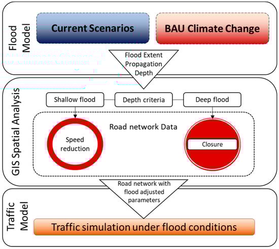
Figure 1.
Loosely coupling flood model outputs with traffic model input parameters (based on methodology outlined by Pyatkova, 2018 [16]).
2.1. Barcelona Research Site
For the Barcelona Case Study, a 1D/2D-coupled flood model that utilizes the dual drainage concept [17] using Infoworks ICM (Intergrated Catchment Modelling) [18] has been employed. This hydrodynamic model was used to provide outputs of both water depths and velocities for different return periods under the present (Baseline) and Future Climate Change scenarios whereby a Business As Usual (BAU) policy is assumed (i.e., no adaptation measures applied within the city). For the climate change scenarios in Barcelona, a Representative Concentration Pathway of 8.5 (RCP8.5) has been considered. Table 1 shows the comparison of the maximum rainfall intensities for the Baseline and BAU scenarios from the synthetic rainfall events generated via the Foundation for Climate Research (FIC) used within the flood model.

Table 1.
Comparison between maximum 5 intensities of Current Scenario (Baseline) and Future Climate Change Scenario (BAU) of synthetic rainfall events used within Barcelona Case Study (Deliverable 2.3 RESCCUE).
2.1.1. Barcelona Traffic Model
Within the city of Barcelona, the Departament d’Estratègia de la Mobilitat has developed/provided a pre-existing meso-scale traffic model using the commercial software package TransCAD® [19]. For this meso-scale traffic model, the road network was divided up into road sections referred to links and each link had a wealth of properties relating both the physical characteristics and imposed rules parameters of the road including, but not limited to speed restrictions, number of parking maneuvers per hour, and lane capacity. Upon addition of all the required parameters within TransCAD®, the model can evaluate how the road network performs. Figure 2 shows the extent of the Barcelona traffic model and the relative speed reductions that are calculated by the model under normal operating (dry weather) conditions. In this figure the %Speed Difference (Equation (1)) refers to the calculated/modelled speed of the vehicles derived from the TransCAD® software, relative to the “Free Flow Speed” (the speed at which a vehicle could move along the section unimpeded by other vehicles). The figure highlights the high levels of congestion within the heart of the city and through the major roadways along the outer perimeter in the modelling result.
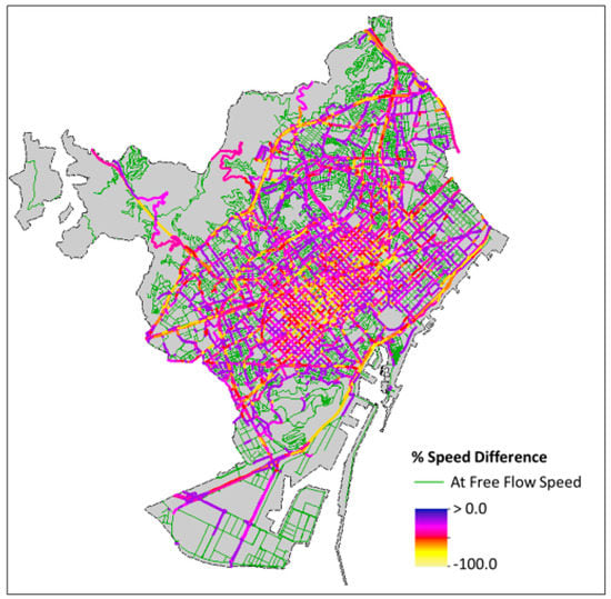
Figure 2.
Percentage speed reduction of traffic in meso-scale model with respect to free-flow speed.
2.2. Bristol Research Site
For the Bristol research site, the Infoworks ICM was also employed at a city-wide level. In contrast to the FIC Climate data used in the Barcelona case, the Bristol case study’s climate data was derived from UKCP09 [9] predictions. Table 2 shows a comparison of the associated rainfall depths of a 1 in 100-year, 60-min duration event for BAU in Bristol based on UKCP09. From this analysis, for a comparative study of pluvial flooding, the upper end (high emissions scenario) and upper epoch (furthest future projection: 2071-2100) were selected for the climate change scenarios as they show a comparative climate change uplift (highlighted in Table 2).
Table 2.
Synthetic rainfall depths from a 1 in 100-year, 60-min duration event derived from UKCP09 climate change projections.
For the Bristol research site, we were limited with the number of return periods available from the flood model outputs. For the Baseline scenarios, we used 1 in 10, 30, and 100-year return periods and for the Future Climate Change scenario, we selected the 1 in 10, 20, and 100-year scenario with the 1 in 20 Year being deemed to be the closest available approximation to the Baseline 1 in 30 year event with climate change uplift applied.
Bristol Traffic Model
Unlike the Barcelona case study, Bristol did not have a pre-existing traffic model available for testing. Due to this, we looked to develop a micro-scale traffic model using the Open Source “Simulating Urban Mobility” (SUMO) software [20]. In contrast to the meso-scale model, the micro-scale model used for Bristol in this analysis simulates the movement of each individual vehicle separately as shown in Figure 3.
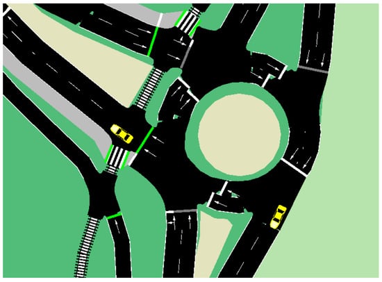
Figure 3.
Example of SUMO micro-simulation.
For the road network the Bristol model has been built using OpenStreetMap (OSM) data [21]. Using SUMO’s “netconvert” tool, OSM data was converted into a network file suitable for use within SUMO that contains road property information including but not limited to, the number of lanes, junctions, and traffic light locations. In the absence of traffic data, the traffic flows within the network were derived via generating Origin-Destination (OD) matrix database using data from the National-Receptor-Database (NRD) [22]. For this process, we assumed vehicles start from either Residential locations or from the boundary of the road network extent (Network Entry Points) (assuming from outside the city) and that the journeys terminate either at a place of work or they leave the network at a boundary (Network Exit Points). Table 3 shows the composition of the origin-destination points with Table 4 showing the percentage distribution of the Origin and Destination locations accordingly. For the ‘School’ classification, some vehicles can use the school as a mid-way point in their journey to simulate school drop-offs during the morning.
Table 3.
Origin Destination points within the road network.
Table 4.
Origin Destination percentage distribution.
Using the spatial information of land-use points from the NRD, SUMO’s ‘Duarouter’ tool was used to generate the OD catalogue of vehicular journeys within the network. An additional rule applied states that each journey must have a journey length equal to or greater than 1 km.
To simulate morning rush hour flows, a sigmoid style curve was used in determining the number of vehicles that were added to the network over time during the simulation. Figure 4 shows the number of vehicles being added to the network over time for a 5000 and 10,100 vehicle scenario respectively using the same curve function.
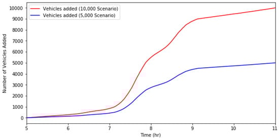
Figure 4.
Number of vehicles added to the network over time for the 5000 and 10,000 traffic volume scenarios.
Figure 5 shows a comparison of the SUMO model outputs for dry weather scenarios, in which the different volumes of traffic present within the network over time whereby vehicles are only being added to the network (starting their journeys) between the hours of 5 am and 11 am. The result demonstrates that a doubling of vehicle journeys from 5000 to 10,000 vehicles within that period results in a seven-fold increase of the number of vehicles present within the network at its peak and a subsequent long tail section as the vehicles leave the network. For both scenarios, between the hours of 7 and 9 am there is a large increase in the number of vehicles being added to the network (approximately 4000 and 8000, respectively). In each scenario, the vehicles added to the network are subsequently removed from the network upon completion of their respective journeys.
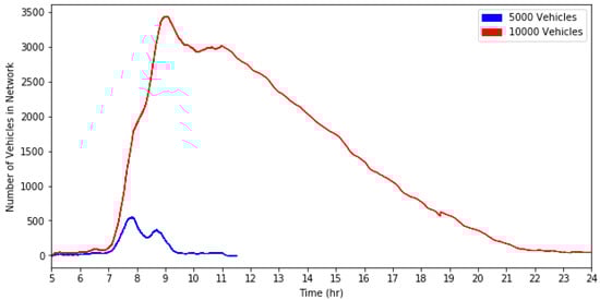
Figure 5.
Comparison of Traffic Volumes in the Network for 5000 journey and 10,000 journey scenarios.
The reason behind this substantial difference in the number of vehicles within the network is a result of traffic jam formation leading to the delay in the completion of vehicle journeys. Figure 6 highlights the variations in the Average Journey Speed (Equation (2)) of vehicles for both the 5000 and 10,000-journey scenarios. The majority of vehicles within the network during the 10,000-journey scenario are travelling at relatively low speeds (less than 10 km/h) whereas the average journey speed for traffic in the 5000-vehicle scenario is around 30 km/h.
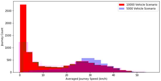
Figure 6.
Average Journey Speed of Vehicles within the Network during the hours of 7 am and 9 am for 5000 and 10,000 journey scenarios.
Figure 7 shows a section within in the network at the peak times (determined in Figure 5) for both journey cases, where the 10,000 journey scenario presents a considerable worse congestion. Because of the congestion both here and in other sections of the network the time for the traffic to clear the network (complete their respective journeys) becomes dependent on the interval timing of the traffic lights and the settings in place within the model “time-to-teleport” to handle these obstruction issues. Traffic signal timing data is often unavailable and has a dominant influence on intersection capacity and network performance [23]. If the timings of these traffics lights are not configured correctly, under high volumes of traffic a stalemate scenario can occur whereby traffic can neither enter nor exit an area thus resulting in severe gridlock. To minimise gridlock scenarios within the traffic model (due to imperfections in the network design) and to deal with instances of vehicles becoming an obstruction, the teleportation rule is applied. In the examples shown in Figure 5, if a vehicle is stationary 40 min (flood duration of 30 min plus and arbitrary 10-min window), it is deemed to be assumed to be erroneously stuck and is teleported to the next edge within its route. Note that it is important that the teleportation rule has a time-limit set to be equal or greater than the duration of a flood event to prevent traffic teleporting past the blocked roads under flooded conditions.
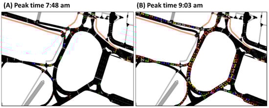
Figure 7.
Comparison of Traffic Volumes at peak times for (A) 5000 journeys and (B) 10,000 journey scenarios.
For the purpose of the study within this paper, we selected 5000 vehicle traffic scenario as a means of analysing the effects of flooding on obstructing or causing diversions to vehicles within the network and to minimise the implications of imperfections in the network configuration itself causing disruptions to traffic flows. Ten 6-h duration traffic scenarios were generated, where each scenario contains 5000 randomly selected journeys from the OD catalog whereby the Origin and Destination’s match the percentage distribution outlined in Table 4. The synthetic sigmoid curve, as shown in Figure 4, was applied to stagger the start times of the vehicles during the simulation to generate a pseudo morning rush scenario. Figure 8 shows the variation/range of the number of vehicles present in the network over time across the ten scenarios, highlighting the two temporal peaks in traffic volumes within the network during the morning rush hours between 7 am and 9 am. Figure 9 shows the extent of the Bristol traffic model and the percentage route distribution of the ten scenarios (10 × 5000 journeys) whereby the higher percentage values correspond to the road sections where vehicles have traversed the most within the 10 scenarios. Here, we observe that within the modelled scenarios, there is a preference for vehicles to traverse the river section (that bisects the city) across the bridges.
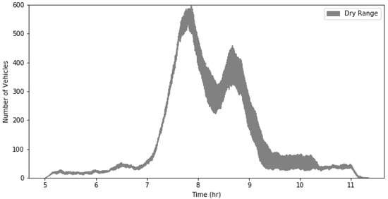
Figure 8.
Range of vehicle distributions from 10 scenarios under dry weather conditions in Bristol road network.
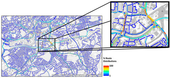
Figure 9.
Percentage Route Distributions under dry conditions.
2.3. Translating Flood Hazards into Traffic Models
To simulate the impacts of flooding within the traffic network the relationship between maximum allowable speeds of vehicles with respect to flood-depths is required. Previous work by Pyatkova et al. [12,13] discretised flood hazards via the relationship of maximum permitted speed limits along road sections with respect to flood depths along those sections. Table 5 shows the discrete ranges for the flood depths, their hazard classification and the subsequent speed reductions along the road sections where these flood depths are present.
Table 5.
Flood hazards’ effect on traffic flows.
Through an intersect analysis, analyzing the depths of water on road surfaces, we modify the input parameters (speed limit) of links within the traffic model. Figure 10 shows an example of the links affected by flooding within Barcelona when analyzing maximum flood-depths of a 1 in 10 year BAU climate change scenario.
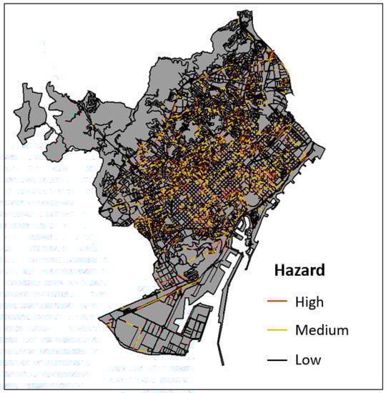
Figure 10.
Example of hazard classification for a 1 in 10 Year Future Climate Change Scenario Event.
2.4. Quantifying Impacts from Traffic Model
The impacts of flooding on traffic flows can be quantified in a number of ways including but not limited to, lost time, fuel consumption and pollution levels. Based on the Multi-Coloured Manual (MCM) [24], we estimated the costs accrued to a vehicle (in GBP) over time and distance in relation to its speed. Table 6 shows a breakdown of costs in pence per unit of speed for five vehicle classes.
Table 6.
Total Costs of travel as a function of speed (pence) [23].
For simplicity in our analysis, we assumed all the vehicles to be of generic petrol driven cars. Figure 11 shows the derived relationship between the estimated costs incurred per car per hour in relation to its speed whereby the line of best fit is described by the function in Equation (3).
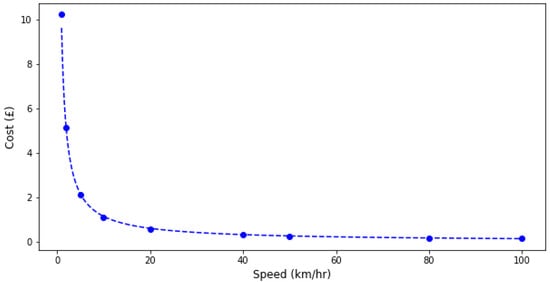
Figure 11.
Derived Cost to Speed relationship Cars based on MCM data.
For the TransCAD® model the accumulated costs were derived from analysing the model outputs at a link level where the total accumulated cost is derived using Equation (4).
where
Traffic VolumeLink = Number of Vehicles per km per hour per link.
LengthLink = Length of link in km.
SFnLink = Calculated cost value with respect to average speed derived via Equation (3).
An estimate of monetary impacts of a flood event with respect to changes in vehicular speed is thus derived via comparing the costs under flooded conditions to the costs under dry weather conditions (Equation (5)).
As the Barcelona model has no temporal information applied to traffic flows, the associated costs were derived with respect to incurred costs per hour of disruption. For the Bristol case study, as we adopted a micro-scale traffic model with a temporal component, the incurred costs were assessed during the period of time the network was deemed to be impacted.
For the Bristol model, data at the link level were also exported but in contrast to the Barcelona model, these outputs vary over time, therefore, Equations (3)–(5) were applied accordingly during the identified period of traffic disruption.
3. Results
3.1. Hazard Analsysis
3.1.1. Barcelona Road Hazards
Figure 12 shows the percentage of road sections that were affected by flood-depths at various return periods for the Baseline (a) and Climate Change (b) scenarios using the rules as described in Table 5. As the severity of the events increases, the number of deep-flooded roads continues to grow whereas the percentage of shallow flooded roads affected begins to level out around 12%. This “levelling out” of the number of shallow flooded sections is due to the transition of road hazard classifications whereby as the severity of the event increases, previously shallow ponding areas upon the surface continue to accumulate flood waters thus moving their flood depths from below 30 cm to 30 cm+ thus transitioning to deep-flooded road status.
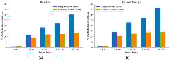
Figure 12.
Affected road sections in Barcelona case study area for (a) Baseline Scenarios, (b) Climate Change Scenarios.
3.1.2. Bristol Road Hazards
Figure 13 shows percentage of affected lane sections for the Bristol case study with respect to the severity of the pluvial flooding events for Baseline (a) and Climate Change (b) scenarios. Within the Bristol case study, an additional criteria specifying the minimum length of a flooded road was included to reduce the number of “flood zones” in the traffic model. This reduction of flood zones was implemented in order improve model performance. In this instance, the minimum length for a flooded road was set to 10 m; therefore, if the length of the section of road that is flooded is less than 10 m, the road will be regarded as not flooded, thereby bringing the overall percentages down. Like that of the Barcelona case study, there is a positive correlation between the severity of the event and the percentage of affected links. For both the Baseline and Climate Change scenarios, we see climbing numbers of affected links and again the transition of shallow flooded areas to deep flooded as the severity of rainfall events increase.
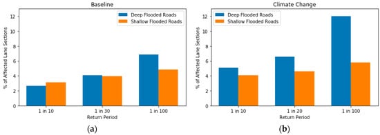
Figure 13.
Affected road sections in the Bristol case study area for (a) Baseline Scenarios, (b) Climate Change Scenarios.
3.2. Impact Assessment
3.2.1. Impacts on Traffic in Barcelona
Upon changing the respective speed limit parameters within TransCAD®, the model was reapplied to assess how the traffic flows within the city have changed. Figure 14 shows speed difference maps calculated from the TransCAD® model runs for a 1 in 100 year event for the Baseline and Climate Change scenarios. Overall appearance shows a similar spatial distribution of speed reductions with slight increases (higher negative values) in reductions for the Climate Change Scenario.
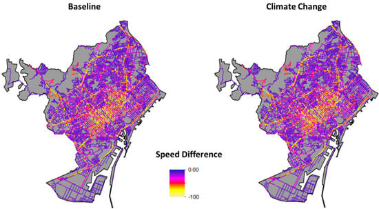
Figure 14.
Comparison of speed differences for 1 in 100-year event for Baseline and Climate Change Scenarios.
Figure 15 shows a comparison of the derived Exceedance Probability (EP) Curves for the Baseline and Future Climate Change prediction scenarios based on summation of all the link cost values. This curve was derived via plotting the total accumulated losses for a pluvial flood event across the network with respect to the probability of occurrence (1/Return Period) of the event. Here, we see that under future climate change conditions the predicted monetary losses/impacts when traffic disruption increases with respect to the severity of the flood event. Table 7 shows a comparison of the loss values with an average increase of monetary losses due to the vehicular speed in the network was reduced by 10% or more under future climate change scenarios.
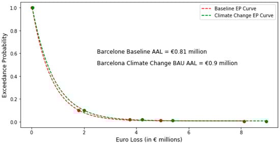
Figure 15.
Flood Impact on Traffic EP Curves for Barcelona.
Table 7.
Monetary losses as a result of traffic speed disruption.
3.2.2. Impacts on Traffic in Bristol
Within the Bristol model, as we also considered the temporal aspect of the flooding in the analyses such that we can specify the time and duration of the flood event. In this example we have specified that flooding occurs as 7 am and lasts for 30 min. During this period, the maximum permitted speeds along hazard affected road sections are temporarily modified and will return to normal at 7:30 am after the flood event has ended.
As the Bristol model is micro-scale, if some journey starts within a flooded region they cannot begin and therefore, are not added to the network this can lead to reduced traffic number on the road during and after the flood event and needs to be considered as part of the impact assessment. Table 8 shows the percentage of journeys whose start-times begin during a flood event and are unable to begin their journey as lie within a closed road.
Table 8.
Journeys unable to begin due to flooding.
One of the additional indicators used to assess the impacts of traffic flows through a micro-scale simulation is to examine the number of vehicles within the network at any given time under flooded conditions and compare this distribution against dry weather conditions. Under flooded conditions, as some road sections will temporarily have their maximum allowable speeds reduced and some sections are temporarily closed. The journey times for vehicles that usually traverse these sections along their assigned routes will increase as vehicles are forced to either move at a reduced speed through shallow water or are diverted onto alternative routes if their original route is obstructed. Figure 15 shows a comparison of the number of vehicles within the road network over time for the different severities of flood events for baseline and future climate change conditions. Within this figure, the “Dry Count Range” represents the range (minimum and maximum) of vehicle counts across the 10 generated OD matrix routing scenarios, and the “Flooded Traffic Count Range” shows the ranges with respect to the network during the 30 min flood simulations. The “Average Flood Traffic Count” represents the average number of vehicles within the network during the respective flood scenarios. The figures highlight that even though a percentage of journeys are lost/unable to start during the flood event, the vehicular saturation of the network both during and immediately after the flood event surpasses the dry weather conditions with the network (on average) recovering by 9 am for all scenarios. The Flooded Traffic Count Range further highlights the different effects flooding has across the 10 generated route scenarios. Figure 16 further shows that even after the flood event has finished the road network still takes time to recover as previously impeded vehicles are continuing to complete their journeys and their remaining presence within the network effects other vehicles that travelling.
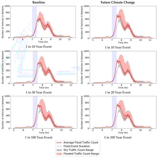
Figure 16.
Comparison of Traffic Network Recovery Times.
Figure 17 shows the comparison of the relative EP curves for the Baseline and Future Climate Change scenarios utilising the same cost to speed relationship applied to the Barcelona case study. Here the points for the Baseline and Climate Change scenarios represent the average calculated losses derived from the simulations with the curves interpolated from these points respectively. Within this example, we are examining the relative cost increases between the hours of 7 am and 9 am that corresponds to the period of disruption shown in Figure 16. In contrast to the Barcelona case study the calculated loss values depicted for Bristol simulations are considerably less. There are a number reasons for this including, but not limited to, the case study area examined within the city of Bristol (24 km2) is considerably smaller than that assessed within Barcelona (102 km2). A second reason relates to the limited number of vehicles used in the duration of the model. With Bristol having a population of approximately 463,500 [25] and 41% of the population driving a car to work [26] the simulated 5000 vehicles over a 6 h period could be a significant under estimate of the traffic volumes/journeys undertaken within the network during this period. The results, therefore, merely serve to show how the effects of climate change can result in observed increases in disruption to traffic flows and potential losses within the traffic network.
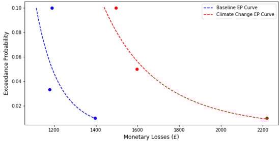
Figure 17.
Flood Impact on Traffic Relative EP Curves for Bristol.
4. Discussion
4.1. Limitations and Assumptions
This paper shows the application of two distinct traffic-modelling approaches with different levels of data availability.
The meso-scale traffic model used in Barcelona case study had very detailed traffic information across the city but the example does not represent the temporal aspect of a flood event. The impact assessment therefore only considers the effects during a flood event and not the recovery period after the event. In addition, within the Barcelona traffic model the criteria for determining hazard classification did not consider the length of the portion of the flooded road, which was an additional restriction applied to the Bristol case study, such that there could be an overestimate of flooded roads. Further assessment could investigate the reduction in perceived flood hazards with the length restriction included.
In contrast to Barcelona’s traffic model, the Bristol model lacked both real traffic-count data and a pre-existing traffic model. Due to these challenges, the traffic model was built from the ground up using freely available Open Source software and data and deriving traffic flows from land-use classifications. As highlighted in Section 2.1.1 there were limitations with this approach when dealing with large traffic volumes and as such the simulations within the paper utilise relatively low traffic counts. For future assessment, a more detailed analysis of the performance of the network could be carried out with the aim of improving/optimising the network under standard dry weather conditions.
For further work and improvements, it would be of interest to see how the micro-scale model performs with real traffic-count data to determine both the volume of traffic over time and the routes/journeys taken by vehicles within the network and determine loss estimates and recovery times under flooded conditions accordingly. Moreover, where such data available, it would be of further interest to evaluate the effectiveness of land-use data for determining route distribution in comparison to real traffic data.
Additionally, in this paper, for the micro-scale simulation we have only considered the flood event occurring with a fixed duration (30 min) starting at one specific time (7 am) which is at the beginning of the rush hour scenario. The degree of disruption to traffic flows within the network would however be dependent upon both when the event occurs and for how long, therefore future work could examine the effects/sensitivity of the time of occurrence and duration parameters.
4.2. Verification of Results
The costs of disruption to traffic flows to cities is generally quite high and within the UK, and has been shown to be within a range of 3–7% of the total accumulated estimated losses from flood events [27]. The flash floods and landslides that occurred as a result of high and prolonged precipitation in Catalonia in September 2006 resulted in the Consorcio de Compensaci´on de Seguros (CCS), the national insurance company paying out €55.9 million and resulted in bringing traffic to a standstill in Barcelona due to jams [28]. In the region of Co. Galway Ireland, the 2015/2016 floods were thought to have losses of €3.8 million of losses through traffic disruption [29]. The calculated losses for these events however are not limited solely to disruption of traffic as a result of standing water but also consider traffic light failures as in the case of Barcelona 2011 [5] and also the road closures due to potential risk to like from flooding. For example, the summer floods of 2007 resulted in the closure of the M1 in the UK for 40 h between junctions 31 and 41 due to the risk of a dam breach and the cost of this disruption alone was estimated to be £2.3 million [6].
The work outlined in this paper shows the potential of combining climate change data with flood mapping and traffic models as a means of assessing the possible implications change may have. For the Barcelona case study, the estimated losses with respect to the measured return periods seem to portray values within the orders of magnitude of similar climate events (as shown in Co. Galway flood event that was a 1 in 100-year event). As the data used for traffic model in the Bristol case study was assumed based on NRD data and with low traffic counts the estimated losses serve more as a benchmark/guide relative to the severity of input flood events to highlight the potential implications of climate change on traffic.
The model, however, highlights the impact of flooding is not limited to the period of time where there is standing water upon the roads surface but also post flood event as the network takes time to recover.
5. Conclusions
Two case studies each with different traffic modelling approaches were presented within this paper. Both cases have differing qualities and sources of input data where one has been derived from traffic counts/surveys within the city and the other approximated from land-use classifications. The two approaches both demonstrate the feasibility of loosely coupling traffic models to flood mapping as a basis of assessing the potential impacts to traffic flows within the city. The Barcelona case study illustrates how changing parameters within the model input data can serve to approximate the effects of flooding within the model. The Bristol case study shows that even with limited data, we can begin to create a traffic model for basic impact assessment that can be built upon within the future. In addition, the micro-scale approach used within the Bristol case study shows the effect of flooding is not solely limited to the duration of the flood and that the impact assessment needs to consider the recovery time of the network.
Author Contributions
The main author B.E. worked on each component of the paper including the conceptualization, methodology, software, modelling, analysis and validation, and original draft. A.G.G. facilitated with the modelling and validation with respect to the Barcelona case study and the review and editing of the paper. S.D., A.S.C., J.W., and J.S. were each involved with the validation processes of the research and the review and editing of the paper. All authors have read and agreed to the published version of the manuscript.
Funding
This research was funded by the European Union’s Horizon 2020 Research and Innovation Programme, RESCCUE project grant number 700174.
Acknowledgments
The author would like to thank Katya Pyatkova for her support with the development of the micro-scale traffic model for the city of Bristol.
Conflicts of Interest
The authors declare no conflict of interest.
References
- Havaei-Ahary, B. Road Traffic Estimates: Great Britain 2018. 2019. Available online: https://assets.publishing.service.gov.uk/government/uploads/system/uploads/attachment_data/file/808555/road-traffic-estimates-in-great-britain-2018.pdf (accessed on 11 March 2020).
- Arrighi, C.; Pregnolato, M.; Dawson, R.J.; Castelli, F. Preparedness against mobility disruption by floods. Sci. Total Environ. 2019, 654, 1010–1022. [Google Scholar] [CrossRef] [PubMed]
- Green, D.; Yu, D.; Pattison, I.; Wilby, R.; Bosher, L.; Patel, R.; Thompson, P.; Trowell, K.; Draycon, J.; Halse, M.; et al. City-Scale Accessibility of Emergency Responders Operating During Flood Events. 2016. Available online: https://repository.lboro.ac.uk/articles/City-scale_accessibility_of_emergency_responders_operating_during_flood_events/9483023 (accessed on 11 March 2020).
- Coles, D.; Yu, D.; Wilby, R.L.; Green, D.; Herring, Z. Beyond ‘flood hotspots’: Modelling emergency service accessibility during flooding in York, UK. J. Hydrol. 2017, 546, 419–436. [Google Scholar] [CrossRef]
- Travieso, J. Una Gran Tormenta Derriba 50 Árboles en Barcelona y Causa Graves Inundaciones. 2011. Available online: https://www.20minutos.es/noticia/1124029/0/inundaciones/barcelona/emergencias/ (accessed on 11 March 2020).
- Chatterton, J.; Viavattene, C.; Morris, J.; Edmund Penning-Rowsell, S.T. The Costs of the Summer 2007 Floods in England. 2010. Available online: http://www.publications.parliament.uk/pa/cm201012/cmselect/cmtran/794/794.pdf (accessed on 11 March 2020).
- Department for Transport. Government Response to the Transport Resilience Review. 2014. Available online: https://assets.publishing.service.gov.uk/government/uploads/system/uploads/attachment_data/file/380211/cm-8968-print.pdf (accessed on 11 March 2020).
- Highways England. Climate Adaptation Risk Assessment Progress Update—2016; Highways England: London, UK, 2016. [Google Scholar]
- Murphy, J.M.; Sexton, D.M.H.; Jenkins, G.J.; Boorman, P.M.; Booth, B.B.B.; Brown, C.C.; Clark, R.T.; Collins, M.; Harris, G.R.; Kendon, E.J.; et al. UK Climate Projections Science Report: Climate Change Projections; Met Office Hadley Centre: Exeter, UK, 2009.
- Martínez-Gomariz, E.; Gómez, M.; Russo, B.; Djordjević, S. Stability criteria for flooded vehicles: A state-of-the-art review. J. Flood Risk Manag. 2018, 11, S817–S826. [Google Scholar] [CrossRef]
- Martínez-Gomariz, E.; Gómez, M.; Russo, B.; Djordjević, S. A new experiments-based methodology to define the stability threshold for any vehicle exposed to flooding. Urban Water J. 2017, 14, 930–939. [Google Scholar] [CrossRef]
- Pyatkova, K.; Chen, A.S.; Butler, D.; Vojinović, Z.; Djordjević, S. Assessing the knock-on effects of flooding on road transportation. J. Environ. Manag. 2019, 244, 48–60. [Google Scholar] [CrossRef] [PubMed]
- Pyatkova, K.; Chen, A.S.; Djordjević, S.; Butler, D.; Vojinović, Z.; Abebe, Y.A.; Hammond, M. Flood impacts on road transportation using microscopic traffic modelling techniques. In Simulating Urban Traffic Scenarios; Behrisch, M., Weber, M., Eds.; Springer International Publishing: Cham, Switzerland, 2019; pp. 115–126. [Google Scholar]
- Pregnolato, M.; Ford, A.; Wilkinson, S.M.; Dawson, R.J. The impact of flooding on road transport: A depth-disruption function. Transp. Res. Part D Transp. Environ. 2017, 55, 67–81. [Google Scholar] [CrossRef]
- Sohn, J. Evaluating the significance of highway network links under the flood damage: An accessibility approach. Transp. Res. Part A Policy Pract. 2006, 40, 491–506. [Google Scholar] [CrossRef]
- Pyatkova, K. Flood Impacts on Road Transportation. Ph.D. Dissertation, University of Exeter, Exeter, UK, 2018. Available online: https://ore.exeter.ac.uk/repository/handle/10871/37346 (accessed on 11 March 2020).
- Djordjević, S.; Prodanović, D.; Maksimović, Č. An approach to simulation of dual drainage. Water Sci. Technol. 1999, 39, 95–103. [Google Scholar] [CrossRef]
- Innovyze. User Manual References, InfoWorks ICM (Integrated Catchment Modeling) v.3.5; Innovyze: Newbury, UK, 2013. [Google Scholar]
- TransCAD Transportation Planning Software. Available online: https://www.caliper.com/tcovu.htm (accessed on 20 December 2019).
- Lopez, P.A.; Behrisch, M.; Bieker-Walz, L.; Erdmann, J.; Flötteröd, Y.; Hilbrich, R.; Lücken, L.; Rummel, J.; Wagner, P.; WieBner, E. Microscopic traffic simulation using SUMO. In Proceedings of the 2018 21st International Conference on Intelligent Transportation Systems (ITSC), Maui, HI, USA, 4–7 November 2018; pp. 2575–2582. [Google Scholar] [CrossRef]
- OpenStreetMap. Available online: https://www.openstreetmap.org/ (accessed on 21 September 2019).
- Find Open Data. Available online: https://data.gov.uk/ (accessed on 21 December 2019).
- Flötteröd, Y.-P.; Behrisch, M. Improving SUMO’s signal control programs by introducing route information. In Proceedings of the SUMO 2018—Simulating Autonomous and Intermodal Transport Systems, Berlin, Germany, 14–16 May 2018; Volume 2, pp. 162–172. [Google Scholar] [CrossRef]
- Penning-Rowsell, E.; Viavattene, C.; Pardoe, J.; Chatterton, J.; Parker, D.; Morris, J. The Benefits of Flood and Coastal Risk Management: A Handbook of Assessment Techniques; Flood Hazard Research Centre, Middlesex University: London, UK, 2010. [Google Scholar]
- Bristol City Council “Population of Bristol”. Available online: https://www.bristol.gov.uk/statistics-census-information/the-population-of-bristol (accessed on 31 January 2020).
- Bristol Is Open “How Do Bristolians Go to Work”. Available online: https://www.bristolisopen.com/how-does-bristol-go-to-work/ (accessed on 31 January 2020).
- Environment Agency. Estimating the Economic Costs of the 2015 to 2016 Winter Floods. 2018. Available online: https://assets.publishing.service.gov.uk/government/uploads/system/uploads/attachment_data/file/672087/Estimating_the_economic_costs_of_the_winter_floods_2015_to_2016.pdf (accessed on 11 March 2020).
- Llasat, M.; López, L.; Barnolas, M.; Llasat-Botija, M. Flash-floods in Catalonia: The social perception in a context of changing vulnerability. Adv. Geosci. 2008, 17. [Google Scholar] [CrossRef]
- McDermot, T.; Kilgarriff, P.; Vega, A.; O’donoghue, C.; Morrisey, M. The indirect economic costs of flooding: Evidence from transport disruptions during Storm Desmond. In Proceedings of the Irish Economic Association Annual Conference 2017, Dublin, Ireland, 4–5 May 2017; Available online: https://iea2017.exordo.com/files/papers/120/initial_draft/commuting-discruption-floods-v5-IEA-submission.pdf (accessed on 11 March 2020).


© 2020 by the authors. Licensee MDPI, Basel, Switzerland. This article is an open access article distributed under the terms and conditions of the Creative Commons Attribution (CC BY) license (http://creativecommons.org/licenses/by/4.0/).