Air Pollution Prediction Using Long Short-Term Memory (LSTM) and Deep Autoencoder (DAE) Models


Abstract
1. Introduction
2. Related Research
3. Materials
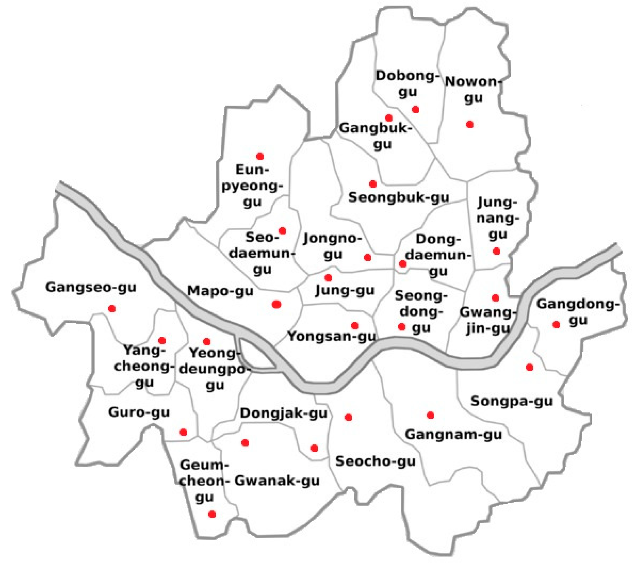
3.1. Study Areas
3.2. Dataset
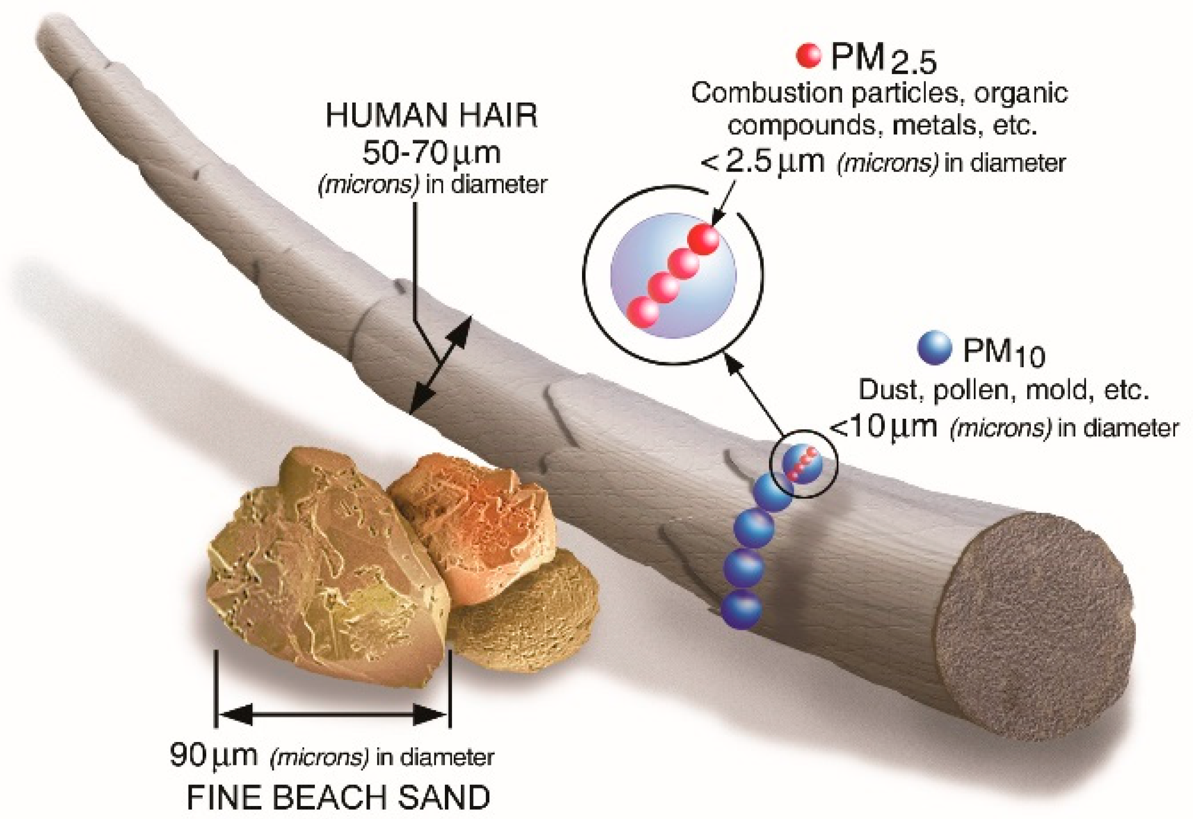
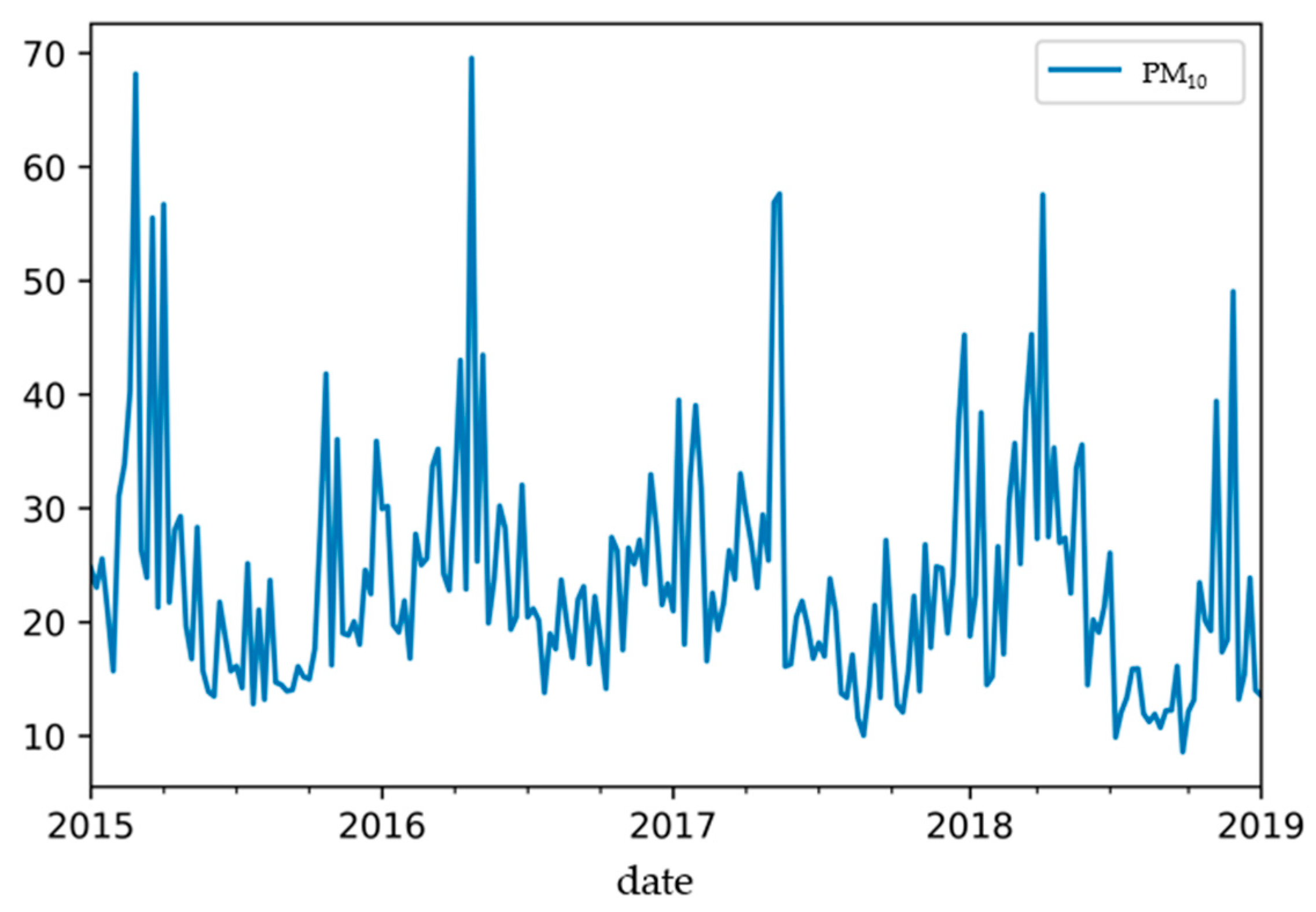
3.2.1. PM Data
3.2.2. Meteorological Data
4. Proposed Methods
4.1. LSTM Models
4.2. Deep Autoencoders (DAEs)
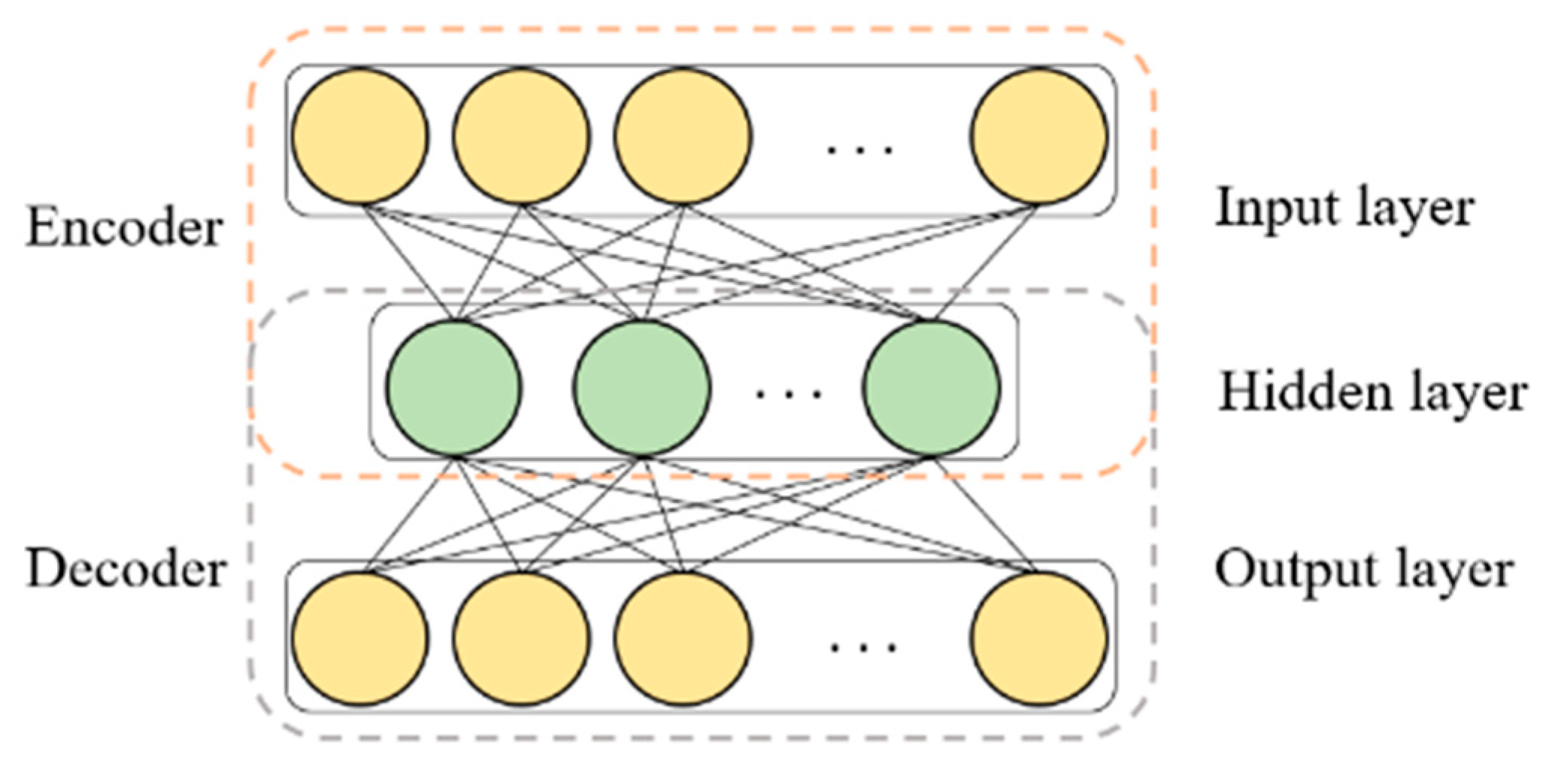
4.2.1. Autoencoder
4.2.2. The DAE Model
4.3. Model Performance Evaluation
5. Results
5.1. Fine PM Prediction
5.2. LSTM Model Performance
5.3. DAE Model Performance
6. Conclusions
Author Contributions
Funding
Acknowledgments
Conflicts of Interest
References
- Jung, W. South Korea’s Air Pollution: Gasping for Solutions. Available online: http://isdp.eu/publication/south-koreas-air-pollution-gasping-solutions/ (accessed on 6 April 2019).
- Jin, L.; Luo, X.; Fu, P.; Li, X.-D. Airborne particulate matter pollution in urban China: a chemical mixture perspective from sources to impacts. Natl. Sci. Rev. 2016, 4, 593–610. [Google Scholar] [CrossRef]
- Xing, Y.-F.; Xu, Y.-H.; Shi, M.-H.; Lian, Y.-X. The impact of PM2.5 on the human respiratory system. J. Thorac. Dis. 2016, 8, E69–E74. [Google Scholar] [PubMed]
- Torrisi, M.; Pollastri, G.; Le, Q. Deep learning methods in protein structure prediction. Comput. Struct. Biotechnol. J. 2020, 521, 436–444. [Google Scholar] [CrossRef]
- Heaton, J. Deep Learning and Neural Networks; Heaton Research Inc: Washington, DC, USA, 2015. [Google Scholar]
- Deng, L.; Yu, D. Deep Learning: Methods and Applications. Found. Trends Signal Process. 2014, 7, 197–387. [Google Scholar] [CrossRef]
- Ordieres-Meré, J.; Vergara, E.; Capuz-Rizo, S.F.; Salazar, R. Neural network prediction model for fine particulate matter (PM2.5) on the US–Mexico border in El Paso (Texas) and Ciudad Juárez (Chihuahua). Environ. Model. Softw. 2005, 20, 547–559. [Google Scholar] [CrossRef]
- Barai, S.V.; Dikshit, A.K.; Sharma, S. Neural Network Models for Air Quality Prediction: A Comparative Study. In Computational Intelligence in Security for Information Systems; Springer Science and Business Media LLC: Berlin/Heidelberg, Germany, 2007; Volume 39, pp. 290–305. [Google Scholar]
- Zhou, Q.; Jiang, H.; Wang, J.; Zhou, J. A hybrid model for PM 2.5 forecasting based on ensemble empirical mode decomposition and a general regression neural network. Sci. Total. Environ. 2014, 496, 264–274. [Google Scholar] [CrossRef]
- Elangasinghe, M.; Singhal, N.; Dirks, K.; Salmond, J.; Samarasinghe, S. Complex time series analysis of PM10 and PM2.5 for a coastal site using artificial neural network modelling and k-means clustering. Atmospheric Environ. 2014, 94, 106–116. [Google Scholar] [CrossRef]
- Russo, A.; Raischel, F.; Lind, P.G. Air quality prediction using optimal neural networks with stochastic variables. Atmos. Environ. 2013, 79, 822–830. [Google Scholar] [CrossRef]
- Hu, X.; Waller, L.A.; Lyapustin, A.; Wang, Y.; Al-Hamdan, M.Z.; Crosson, W.L.; Estes, M.G., Jr.; Estes, S.M.; Quattrochi, D.; Puttaswamy, S.J.; et al. Estimating ground-level PM2.5 concentrations in the Southeastern United States using MAIAC AOD retrievals and a two-stage model. Remote. Sens. Environ. 2014, 140, 220–232. [Google Scholar] [CrossRef]
- Chang, Y.-S.; Lin, K.-M.; Tsai, Y.-T.; Zeng, Y.-R.; Hung, C.-X. Big data platform for air quality analysis and prediction. In Proceedings of the 2018 27th Wireless and Optical Communication Conference (WOCC), Hualien, Taiwan, 30 April–1 May 2018; pp. 1–3. [Google Scholar]
- Schmidhuber, J. Deep learning in neural networks: An overview. Neural Networks 2015, 61, 85–117. [Google Scholar] [CrossRef]
- Kalapanidas, E.; Avouris, N. Short-term air quality prediction using a case-based classifier. Environ. Model. Softw. 2001, 16, 263–272. [Google Scholar] [CrossRef]
- Athanasiadis, I.N.; Kaburlasos, V.G.; Mitkas, P.A.; Petridis, V. Applying machine learning techniques on air quality data for real-time decision support. In Proceedings of the First international NAISO symposium on information technologies in environmental engineering (ITEE’2003), Gdansk, Poland, 24–27 June 2003. [Google Scholar]
- Famoso, F.; Wilson, J.; Monforte, P.; Lanzafame, R.; Brusca, S.; Lulla, V. Measurement and modeling of ground-level ozone concentration in Catania, Italy using biophysical remote sensing and GIS. Int. J. Appl. Eng. Res. 2017, 12, 10551–10562. [Google Scholar]
- Hoek, G.; Beelen, R.; de Hoogh, K.; Vienneau, D.; Gulliver, J.; Fischer, P.; Briggs, D. A review of land-use regression models to assess spatial variation of outdoor air pollution. Atmos. Environ. 2008, 42, 7561–7578. [Google Scholar] [CrossRef]
- Lee, J.-H.; Wu, C.-F.; Hoek, G.; De Hoogh, K.; Beelen, R.; Brunekreef, B.; Chan, C.-C. Land use regression models for estimating individual NOx and NO2 exposures in a metropolis with a high density of traffic roads and population. Sci. Total. Environ. 2014, 472, 1163–1171. [Google Scholar] [CrossRef] [PubMed]
- Qi, Y.; Li, Q.; Karimian, H.; Liu, D. A hybrid model for spatiotemporal forecasting of PM2.5 based on graph convolutional neural network and long short-term memory. Sci. Total. Environ. 2019, 664, 1–10. [Google Scholar] [CrossRef] [PubMed]
- Singh, K.P.; Gupta, S.; Rai, P. Identifying pollution sources and predicting urban air quality using ensemble learning methods. Atmos. Environ. 2013, 80, 426–437. [Google Scholar] [CrossRef]
- Corani, G. Air quality prediction in Milan: feed-forward neural networks, pruned neural networks and lazy learning. Ecol. Model. 2005, 185, 513–529. [Google Scholar] [CrossRef]
- Fu, M.; Wang, W.; Le, Z.; Khorram, M.S. Prediction of particular matter concentrations by developed feed-forward neural network with rolling mechanism and gray model. Neural Comput. Appl. 2015, 26, 1789–1797. [Google Scholar] [CrossRef]
- Jiang, D.; Zhang, Y.; Hu, X.; Zeng, Y.; Tan, J.; Shao, D. Progress in developing an ANN model for air pollution index forecast. Atmos. Environ. 2004, 38, 7055–7064. [Google Scholar] [CrossRef]
- Qin, D.; Yu, J.; Zou, G.; Yong, R.; Zhao, Q.; Zhang, B. A Novel Combined Prediction Scheme Based on CNN and LSTM for Urban PM2.5 Concentration. IEEE Access 2019, 7, 20050–20059. [Google Scholar] [CrossRef]
- Bui, T.-C.; Le, V.-D.; Cha, S.-K. A Deep Learning Approach for Forecasting Air Pollution in South Korea Using LSTM 2018. arXiv 2018, arXiv:1804.07891. [Google Scholar]
- Zhao, J.; Deng, F.; Cai, Y.; Chen, J. Long short-term memory—Fully connected (LSTM-FC) neural network for PM2.5 concentration prediction. Chemosphere 2019, 220, 486–492. [Google Scholar] [CrossRef] [PubMed]
- Reddy, V.; Yedavalli, P.; Mohanty, S.; Nakhat, U. Deep Air: Forecasting Air Pollution in Beijing, China. arXiv 2018. [Google Scholar]
- Kim, S.; Lee, J.M.; Lee, J.; Seo, J. Deep-dust: Predicting concentrations of fine dust in Seoul using LSTM 2019. arXiv 2019. [Google Scholar]
- Li, X.; Peng, L.; Hu, Y.; Shao, J.; Chi, T. Deep learning architecture for air quality predictions. Environ. Sci. Pollut. Res. 2016, 23, 22408–22417. [Google Scholar] [CrossRef]
- Lv, Y.; Duan, Y.; Kang, W.; Li, Z.; Wang, F.-Y. Traffic Flow Prediction With Big Data: A Deep Learning Approach. IEEE Trans. Intell. Transp. Syst. 2014, 16, 1–9. [Google Scholar] [CrossRef]
- Huang, W.; Song, G.; Hong, H.; Xie, K. Deep Architecture for Traffic Flow Prediction: Deep Belief Networks With Multitask Learning. IEEE Trans. Intell. Transp. Syst. 2014, 15, 2191–2201. [Google Scholar] [CrossRef]
- Teng, Y.; Huang, X.; Ye, S.; Li, Y. Prediction of particulate matter concentration in Chengdu based on improved differential evolution algorithm and BP neural network model. In Proceedings of the 2018 IEEE 3rd International Conference on Cloud Computing and Big Data Analysis (ICCCBDA), Institute of Electrical and Electronics Engineers (IEEE), Chengdu, China, 20–22 April 2018; pp. 100–106. [Google Scholar]
- Dong, Y.; Wang, H.; Zhang, L.; Zhang, K. An improved model for PM2.5 inference based on support vector machine. In Proceedings of the 2016 17th IEEE/ACIS International Conference on Software Engineering, Artificial Intelligence, Networking and Parallel/Distributed Computing (SNPD), Institute of Electrical and Electronics Engineers (IEEE), Shanghai, China, 30 May–1 June 2016; pp. 27–31. [Google Scholar]
- Air Korea. Available online: http://www.airkorea.or.kr/web (accessed on 6 April 2019).
- Korea Meteorological Agency. Available online: https://data.kma.go.kr/cmmn/main.do (accessed on 6 April 2019).
- Mahata, S.K.; Das, D.; Bandyopadhyay, S. MTIL2017: Machine Translation Using Recurrent Neural Network on Statistical Machine Translation. J. Intell. Syst. 2019, 28, 447–453. [Google Scholar] [CrossRef]
- Wang, Q.; Lin, J.; Yuan, Y. Salient Band Selection for Hyperspectral Image Classification via Manifold Ranking. IEEE Trans. Neural Networks Learn. Syst. 2016, 27, 1279–1289. [Google Scholar] [CrossRef]
- Graves, A.; Mohamed, A.-R.; Hinton, G.; Graves, A. Speech recognition with deep recurrent neural networks. In Proceedings of the 2013 IEEE International Conference on Acoustics, Speech and Signal Processing, Institute of Electrical and Electronics Engineers (IEEE), Vancouver, BC, Canada, 26–31 May 2013; pp. 6645–6649. [Google Scholar]
- Milan, A.; Rezatofighi, S.H.; Dick, A.; Reid, I.; Schindler, K. Online Multi-Target Tracking Using Recurrent Neural Networks. arXiv 2016, 1604, 03635. [Google Scholar]
- Liu, T.; Wu, T.; Wang, M.; Fu, M.; Kang, J.; Zhang, H. Recurrent Neural Networks based on LSTM for Predicting Geomagnetic Field. In Proceedings of the 2018 IEEE International Conference on Aerospace Electronics and Remote Sensing Technology (ICARES), Institute of Electrical and Electronics Engineers (IEEE), Bali, Indonesia, 20–21 September 2018; pp. 1–5. [Google Scholar]
- Chung, J.; Gulcehre, C.; Cho, K.; Bengio, Y. Empirical Evaluation of Gated Recurrent Neural Networks on Sequence Modeling. arXiv 2014, 1412, 3555. [Google Scholar]
- Fan, J.; Li, Q.; Hou, J.; Feng, X.; Karimian, H.; Lin, S. A Spatiotemporal Prediction Framework for Air Pollution Based on Deep RNN. ISPRS Ann. Photogramm. Remote. Sens. Spat. Inf. Sci. 2017, 4, 15–22. [Google Scholar] [CrossRef]
- Xu, G.; Fang, W. Shape retrieval using deep autoencoder learning representation. In Proceedings of the 2016 13th International Computer Conference on Wavelet Active Media Technology and Information Processing (ICCWAMTIP), Institute of Electrical and Electronics Engineers (IEEE), Chengdu, China, 16–18 December 2016; pp. 227–230. [Google Scholar]
- Zhao, X.; Nutter, B. Content Based Image Retrieval system using Wavelet Transformation and multiple input multiple task Deep Autoencoder. In Proceedings of the 2016 IEEE Southwest Symposium on Image Analysis and Interpretation (SSIAI), Santa Fe, NM, USA, 6–8 March 2016; pp. 97–100. [Google Scholar]


| AQI | Description | |
|---|---|---|
| PM10 | PM2.5 | |
| 0–30 | 0–15 | Good |
| 31–50 | 16–25 | Moderate |
| 51–100 | 26–50 | Unhealthy |
| 100+ | 50+ | Hazardous |
| Step | Description |
|---|---|
| 1 | Preprocessing of all fine particulate matter and meteorological data |
| 2 | LSTM pre-training
|
| 3 | Fine tuning
|
| 4 | Obtain prediction results |
| Step | Description |
|---|---|
| 1 | Preprocessing of all fine particulate matter and meteorological data |
| 2 | Preparation of the DAE framework
|
| 3 | Fine tuning
|
| 4 | Obtain prediction results |
| Batch Size | Learning Rate | Epoch | RMSE | Processing Time (Min) | |
|---|---|---|---|---|---|
| PM10 | PM2.5 | ||||
| 32 | 0.01 | 100 | 11.113 | 12.174 | 11:18 |
| 64 | 0.01 | 100 | 11.163 | 12.237 | 17:05 |
| 128 | 0.01 | 100 | 11.139 | 12.243 | 23:57 |
| 256 | 0.01 | 100 | 11.228 | 11.642 | 38:18 |
| Batch Size | Learning Rate | Epoch | RMSE | Processing Time (Min) | |
|---|---|---|---|---|---|
| PM10 | PM2.5 | ||||
| 32 | 0.01 | 100 | 15.644 | 17.493 | 11:50 |
| 64 | 0.01 | 100 | 15.038 | 15.437 | 15:40 |
| 128 | 0.01 | 100 | 16.024 | 15.711 | 24:05 |
| 256 | 0.01 | 100 | 16.825 | 17.473 | 35:58 |
© 2020 by the authors. Licensee MDPI, Basel, Switzerland. This article is an open access article distributed under the terms and conditions of the Creative Commons Attribution (CC BY) license (http://creativecommons.org/licenses/by/4.0/).
Share and Cite
Xayasouk, T.; Lee, H.; Lee, G. Air Pollution Prediction Using Long Short-Term Memory (LSTM) and Deep Autoencoder (DAE) Models. Sustainability 2020, 12, 2570. https://doi.org/10.3390/su12062570
Xayasouk T, Lee H, Lee G. Air Pollution Prediction Using Long Short-Term Memory (LSTM) and Deep Autoencoder (DAE) Models. Sustainability. 2020; 12(6):2570. https://doi.org/10.3390/su12062570
Chicago/Turabian StyleXayasouk, Thanongsak, HwaMin Lee, and Giyeol Lee. 2020. "Air Pollution Prediction Using Long Short-Term Memory (LSTM) and Deep Autoencoder (DAE) Models" Sustainability 12, no. 6: 2570. https://doi.org/10.3390/su12062570
APA StyleXayasouk, T., Lee, H., & Lee, G. (2020). Air Pollution Prediction Using Long Short-Term Memory (LSTM) and Deep Autoencoder (DAE) Models. Sustainability, 12(6), 2570. https://doi.org/10.3390/su12062570