Abstract
Depth‒damage curves, also known as vulnerability curves, are an essential element of many flood damage models. A relevant characteristic of these curves is their applicability limitations in space and time. The reader will find firstly in this paper a review of different damage models and depth‒damage curve developments in the world, particularly in Spain. In the framework of the EU-funded RESCCUE project, site-specific depth‒damage curves for 14 types of property uses have been developed for Barcelona. An expert flood surveyor’s opinion was essential, as the occasional lack of data was made up for by his expertise. In addition, given the lack of national standardization regarding the applicability of depth‒damage curves for flood damage assessments in Spanish urban areas, regional adjustment indices have been derived for transferring the Barcelona curves to other municipalities. Temporal adjustment indices have been performed in order to modify the depth‒damage curves for the damage estimation of future flood events, too. This study attempts to provide nationwide applicability in flood damage reduction studies.
1. Introduction
According to the European Environment Agency (EAA) [1], the total reported economic losses in Europe caused by weather and climate-related extremes over the period 1980–2017 amounted to approximately EUR 453 billion; the losses in Spain amounted to EUR 37 billion. In the words of the Spanish Insurance Compensation Consortium (CCS, for its acronym in Spanish), it is estimated that around 50% of the damage was covered by insurance in Spain. For example, the total losses from the Lorca earthquake in 2011 were estimated at EUR 1 billion, EUR 0.5 billion of which was insured and thus compensated [2]. Nowadays, economic losses from flood events at the urban level are increasingly relevant, in line with socioeconomic changes such as population growth and the expansion of infrastructure density in cities around the world [3]. Floods are the most damaging natural hazard in Europe, with around two-thirds of the total damage costs. Moreover, rising temperatures are expected to intensify the hydrological cycle, thus leading to more frequent and intense floods in many regions, together with a corresponding increase in economic losses. Nevertheless, it has to be noted that increases in costs from flooding in recent decades can be partly attributed to more people living in flood-prone areas [4].
The types of damage caused by floods are numerous and can be classified as tangible and intangible; these, in turn, can be categorized as direct or indirect [5]. Traditionally, economic flood damage assessment (i.e., direct damage) concerning flood impacts has been studied in more depth. Particularly in urban areas, the focus has been on damage caused to flooded properties. Thus, a variety of methodologies, which still need more development, have led to important advancements.
Gilbert F. White (1945) [6] was a pioneer in considering the damage to properties. Among other aspects, White [6] defined in greater detail the types of losses in urban areas when a flood occurs, such as those related to properties and shops. His study addressed losses that can occur in residential areas, such as to the foundations and structure of dwellings and other buildings, garages, and vehicles. Also, the loss of property rental income (i.e., indirect damage) was considered. A relevant statement in White’s [6] work was that water depth and velocity variables established the degree of severity of damage to the foundation and structure of dwellings. Water depth was stated to be the most limiting factor for such losses. Although White [6] did not distinguish directly between direct and indirect damage, both categories were addressed in his study.
In Spain, the Directorate General for Civil Defense and Emergencies, and the Spanish Insurance Compensation Consortium (Consorcio de Compensación de Seguros, CCS) have reported that flooding has caused the death of 312 people over the last 20 years, and economic damage amounting to EUR 800 million per annum [7]. In this context, European Directive 2007/60/CE on the assessment and management of flood risks [8] was published, and enacted by the Royal Decree 903/2010 on flood risk evaluation and management [9] in the Spanish legislation. It requires the Member States to develop, adopt, and implement flood risk management plans. These plans encompass a number of measures that involve land management and urban planning, civil protection, insurance, early warning, and improving the condition of rivers and coastal areas. One of the measures included in these plans was the development of guidelines to reduce the vulnerability of properties exposed to floods [7]. The main aim of these guidelines was to improve knowledge of flood consequences and foster citizens’ commitment to risk reduction, focusing on the vulnerability of people and assets and enhancing the resilience of high risk properties.
Although measures to increase buildings’ resilience have been proposed, these plans are focused on riverine floods, which indeed involve important risks that must be dealt with, but only for those urban areas located in flood-prone areas. However, sewer flooding should not be underestimated since all cities are prone to this type of flooding once a drainage system exceeds its design capacity, regardless of the distance to rivers. This type of flood is also expected to become more frequent due to the effects of climate change [10], increasing risk, damage, and disruptions to citizens.
In the framework of the RESCCUE project, tailored depth‒damage curves for Barcelona have been developed. These curves encompass 14 different types of properties that are usually found in highly urbanized areas. There is no standardization at a national level regarding the employment of depth‒damage curves for flood damage assessment. Therefore, this study attempts to bridge the gap in the inability to compare flood damage reduction studies from different Spanish regions. Ultimately, it expects to provide a tool to carry out homogeneously nationwide flood damage assessments. To do so, regional adjustment indices have been derived for transferring the Barcelona curves to other Spanish municipalities. Moreover, temporal adjustment indices have been performed to modify the depth‒damage curves for the damage estimation of future flood events.
This paper offers in Section 2 a review of a variety of flood damage models and depth‒damage curves that can be found within the literature, grouped according to their geographical application: a) worldwide or b) Spain-specific. Section 3 presents the particular context of pluvial floods in Barcelona, the role of the Spanish public insurance company (CCS), and the methodology applied in this study. The data used, its analysis and the processes to create semi-empirical depth‒damage curves tailored to Barcelona are described. The procedure to transfer them in space and time is presented in this section. In Section 4, the relative depth‒damage curves are presented together with their monetization for Barcelona city. Moreover, depth‒damage curves for the most damaged municipalities in Spain due to flooding (pluvial and fluvial) for the 2020 reference year are presented. Finally, Section 5 recaps the main messages of this study, and the usefulness and adequacy of the proposed depth‒damage curves for Spanish cities are argued.
2. Literature Review and Analysis
Even though there is currently no universally trusted system for assessing flood damage in urban areas, most damage models rely on depth‒damage curves (also known as stage‒damage functions) for simplicity [11]. In order to apply damage models to assess the economic impact of flooding over urban areas, the required floodwater depths across the inundated area are usually obtained from 2D simulations [12]. In this section, some of the most relevant damage models worldwide are presented together with a variety of depth‒damage curves developed for regions across the world and those specifically developed for Spanish regions.
2.1. Flood Damage Models
Different approaches have been adopted worldwide in order to develop models to assess damage due to flooding. However, all share a common purpose: evaluating the cost-effectiveness of projects designed to alleviate flood impacts.
In the USA, two well-known models are currently being used to assess the damage caused by floods and other natural hazards. The first is HAZUS-MH [13], which is a multihazard estimation model developed by the U.S. Federal Emergency Management Agency (FEMA) that assesses the impacts of earthquakes, wind, and floods. It was mainly developed by the U.S. National Flood Insurance Program (NFIP), because the insurance industry plays a key role when it comes to natural hazards. The outputs of the damage module are area-weighted estimates of damage as a percentage of replacement cost, at the Census Block or for a given building. Since the U.S. NFIP pays claims based on depreciated value, the model considers depreciation as opposed to cost of repair as the general measure of economic loss. The damage assessment model includes a library of more than 900 damage curves estimating damage to various types of buildings and infrastructure. Some drawbacks of this model are the complexity of the data input process and the U.S. regional-based stage‒damage curves. The second well-known model is HEC-FDA [14], developed by the U.S. Army Corps of Engineers (USACE), which is a freely downloadable software provided together with the rest of the Hydrologic Engineering Center (HEC) resources, and includes extensive documentation. Among its several features, it stores hydrologic and economic data necessary for analysis, provides tools to visualize data and results, and computes expected annual damage. Generic depth‒damage relationships are provided to be utilized for a flood damage study conducted in the USA, in the absence of regionally developed relationships.
A comprehensive study conducted by Jongman et al. [15] compares seven different damage models developed for a variety of regions across Europe and the United States: FLEMO (Germany), Damage Scanner (Netherlands), the Rhine Atlas (Rhine Basin), the Flemish Model (Belgium), Multi-Coloured Manual (MCM) (United Kingdom), HAZUS-MH (United States), and the JRC (Germany, European Commission/HKV). The fact that five out of the seven models are based on aggregated land use data (e.g. CORINE) rather than individual objects (HAZUS-HM and MCM) indicates that the scale of work is an essential matter when either selecting or developing a damage model. Moreover, it should be noted that only two out of the seven models are based on individual objects, which indicates the complexity of developing such detailed damage models. While the object-based models can control for varying building density in areas with same CORINE land use, the area-based models can be applied for rapid calculations over larger areas. However, object-based models such as HAZUS-MH and MCM use a large number of object types and corresponding flood damage characteristics [16]. FLEMO, HAZUS-MH, and the Rhine Atlas models are empirically based and could be more accurate when applied to similar case studies. The others are mainly synthetic with the intrinsic issue of their unreliable application to another region or country. An essential improvement in these recent damage models is their GIS-based characteristic; however, the complexity of the data input process, together with the inherent regional (USA) dependency of depth‒damage curves, may be considered as important drawbacks.
As Jongman et al. [15] noted, the use of depth‒damage curves involves great uncertainty, which makes the models very sensitive. The need to adjust asset values to the regional economic situation and property characteristics when using aggregated land use data was also highlighted by Jongman et al. [15]. In addition, the actual damage to a property is not only due to floodwater depth, but also to factors such as the time of the year the flood occurs, flood duration, water velocity, suspended debris, or warning time. Therefore, there is an intrinsic uncertainty to depth‒damage approaches and a known influence of these other factors on the extent and severity of flood damage to buildings and their contents. However, it is a general practice to accept the water level as a fundamental criterion for estimating the damage caused by these events. Lately, other factors beyond the water level have been incorporated into so-called multiparameter damage models; nonetheless, such models require more complex and extensive datasets [17].
Next, we will present descriptions of a variety of depth‒damage curves developed for different parts of the world, and a more in-depth analysis of those performed for Spanish regions.
2.2. Depth‒Damage Curves in the World
Within damage models, depth‒damage curves, also known as vulnerability curves, are used to represent the vulnerability of elements at risk. These can be found in either a relative or an absolute form, by considering percentages of the total property value or damage expressed in monetary terms, respectively. While relative curves are more transferable in space and time, since they do not depend on the market value of assets, absolute curves need a periodic recalibration to incorporate depreciation and inflation. In addition, depth‒damage curves can be classified by their development process, namely analytical, empirical, and synthetic, and a combination of these could also be possible. The first group (analytical) are laboratory-based curves, where the effect of flood variables, such as depth, velocity, or duration, is assessed through monitoring. Empirical curves are developed through the collection of properties’ damage data by means of survey campaigns. Synthetic functions are derived from the study of a theoretical standard property, assuming that all properties within the studied area are similar. This last type of curve is proposed when no actual data are available. Within the literature, other approaches have been found in terms of classification of the curves, such as by land use, building structure type, building contents or inventory, social status (income level), duration of flood, and warning time. Moreover, curves for buildings (i.e., structures) and contents are usually provided separately.
An important collection of damage curves is provided by the HAZUS-MH model, which offers to users the Federal Insurance Administration’s (FIA) “credibility weighted” depth‒damage curves and selected curves developed by various districts of the U.S. Army Corps of Engineers (USACE). The latter group is included in the HEC-FDA model and described in the Economic Guidance Memorandum (EGM) 04-01 developed by the USACE [18], with the purpose of providing guidance for the use of generic depth‒damage curves in their flood damage reduction studies. These are developed based on actual flood losses in various parts of the United States (from 1996 to 2001) in the framework of the Flood Damage Data Collection Program, aiming at providing Corps districts’ offices with standardized relationships for estimating flood damage. These cover one-story homes, two- or more story homes, and split-level homes, all of them with or without basements.
More recently, Huizinga et al. [19], as one of the JRC technical reports, carried out work to provide a methodology and a database of depth‒damage functions for a variety of assets and land use classes (i.e., residential, commercial, industrial, transport, infrastructure, and agriculture). This work is based on an extensive literature survey to normalize damage curves for each continent at a national scale. The purpose of this work was trying to bridge the gap on the inability to compare flood damage assessments from different countries. The variety of depth‒damage curves developments across countries is displayed in Table 1, at a national level, and Table 2 at a regional level. These tables summarize the main characteristics and sources of depth‒damage curves found in the literature.

Table 1.
Relative depth‒damage curves at a national level.
Table 2.
Relative depth‒damage curves at a regional level.
For comparison purposes, a variety of European residential relative depth‒damage curves [19] have been represented together in the graph in Figure 1.
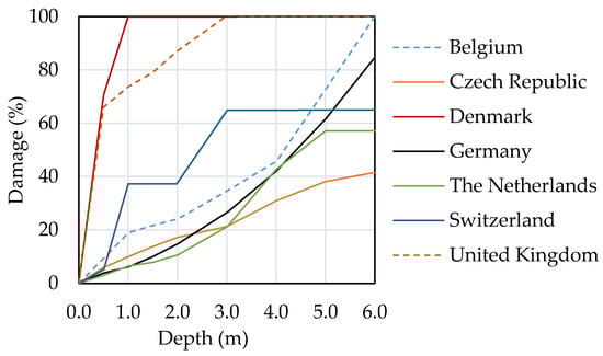
Figure 1.
Residential depth‒damage curves for European countries proposed by Huizinga et al. [19].
As can be observed, there is no correlation between the economic development and the estimated damage percentage of the countries. For instance, the curves developed for the Netherlands present the lowest estimated damage percentage, while it ranks third on GDP per capita of the countries listed [41]. This could be attributed to the level of investment in adaptation measures against flood events of in Netherlands [42], causing lower potential flood event damage compared to other countries. Such dispersion of damage among curves in different European regions was also highlighted by Velasco et al. [5], where seven different types of curves for residential and commercial uses were compared.
2.3. Depth‒Damage Curves in Spain
Only a few recent depth‒damage curves’ developments have been found for Spain, almost all of them addressing specific regions and only one providing national coverage. In 2013, in the framework of a Flood Defense Master Plan for the Spanish region of Marina Baja (Alicante), relative depth‒damage curves for the different CORINE land uses in the region studied [43] were developed. The curves were validated based on actual damage data (i.e., claims paid) provided by the Spanish Insurance Compensation Company, CCS hereafter, and the City Councils of the region studied. Only one month later, in July 2013, the Ministry of Agriculture, Fisheries and Food published the report “Propuesta de mínimos para la metodología de realización de los mapas de riesgo de inundación” [44] (proposal for a common methodology of flood risk maps development). The purpose of this document was to offer a common framework to implement the Directive 2007/60/EC on the assessment and management of flood risks in Spain, and a nationwide relative depth‒damage curve was proposed. It was based on the flood damage caused in the Spanish Ebro basin. Only four water levels were considered, assuming total damage (i.e., 100%) when the water depth exceeds 2 m, and 20% for depths lower than 30 cm. The single curve did not distinguish among land uses, although a table to monetize (€/m2) it according to different land uses was provided.
In 2015, an updated version of the former Flood Risk Prevention Territorial Action Plan for the Spanish Autonomous Community of Valencia (PATRICOVA) [45] was published. Again, a single relative depth‒damage curve was provided, not distinguishing by type of land uses either. It stated that, regardless of the type of land use flooded, below 80 cm of water depth low damage were expected; however, once the water level exceeds this value, the damage increases rapidly up to a depth of 1.2 m, when the increase levels off. Finally, the River Basin Management Plan produced by the Eastern Cantabrian Spanish River Basin District [46], part of the requirements of the Directive 2007/60/EC, has been reviewed. A single relative depth‒damage curve is found in this Plan, which is the result of averaging others developed for other countries, such as the USA (FEMA) and the United Kingdom (Flood Hazard Research Centre). The monetization of these curves is conducted by providing the maximum estimated value per land use. Unlike previous developments, in this case building and contents are differentiated. It considers a percentage from the building damage to constructing the contents’ depth‒damage curve. All reviewed depth‒damage curves for Spanish regions have been jointly graphed and are presented in Figure 2.
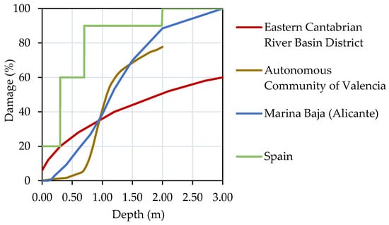
Figure 2.
Depth‒damage curves for Spanish regions.
Ritter et al. [47] conducted a flood damage assessment for the Spanish municipality of Agramunt, in which the depth‒damage curves for Spain were selected from the database provided by Huizinga et al. [19]. It was concluded that the total computed damage for an actual riverine flood event was clearly overestimated after being compared with the claims paid by the Spanish Insurance Compensation Consortium (CCS). This may indicate that the depth‒damage curves employed for the study could overestimate individual assets.
Although there might be other curves developed regionally in Spain, the review conducted has been considered enough to identify the great variety of approaches taken. As observed in Figure 2, where residential and general depth‒damage curves are represented together, the damage for the same water depth varies significantly. For instance, a water depth of 2 m would suggest total damage if the nationwide curve is applied, and only 52% of total damage for the ones developed for the region of Marina Baja. Low water depths would also provide a very different level of damage depending on the curve selection. While the nationwide curve starts from 20% damage, the Marina Baja region curve does not rise above zero until a 10 cm water depth. This is assumed to be the average height of pavement curbs. Moreover, some of them aggregate building and contents (i.e., furniture and household furnishings) damage, while others consider them separately.
3. Materials and Methods
3.1. Context of Pluvial Floods in Barcelona
From 1996 to 2018, pluvial floods in Barcelona alone have required more than EUR 34 million in compensation for industries, offices, dwellings, vehicles, and civil works, according to the Spanish insurance company CCS (Figure 3). The CCS is a state-owned enterprise attached to the Ministry of Economy Affairs and Digital Transformation that performs several complementary functions in the Spanish Insurance Industry, enhancing its stability and protecting the insured. In 2018, four heavy rainfalls hit Barcelona, which caused extraordinary damage (Figure 3 and Figure 4). In 1999 and 2002 alone, the total amount of compensatory damage exceeded that of 2018. It has to be noted, however, that since 2002 several improvements in the drainage network have been carried out. The analysis of these insurance payouts according to the CCS classification (Figure 3b) shows that in 2018 almost 75% of the total payouts were due to damage to commercial buildings, warehouses, and other types. This pattern is common in the last 22 years, representing more than 50% of the total payouts per event, which indicates the vulnerability to pluvial floods of commercial properties in urban areas.
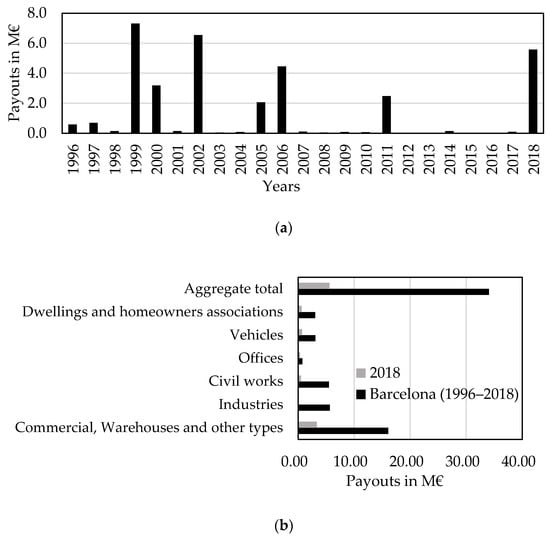
Figure 3.
CCS’s payouts due to damages caused by pluvial floods in Barcelona: (a) historical total annual amounts (1996 to 2018); (b) total historic (22 years) amounts grouped into diverse types of properties, according to CCS classification.
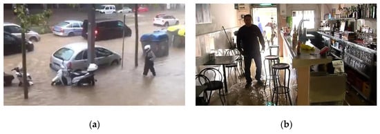
Figure 4.
Consequences of pluvial floods that occurred in Barcelona on (a) 9 October 2018, and (b) 15 November 2018. Sources: a) https://www.elperiodico.com, and b) https://www.telecinco.es.
These figures clearly indicate the relevance of the ever more frequent pluvial floods, highlighting the need to provide tools to estimate the damage that future flood events may cause in urban areas. The existing methodologies to assess flood damage in urban areas are usually based on the use of so-called depth‒damage curves. As described in previous sections, these are merely the mathematical relationship between the floodwater depth reached in the property and the economic damage caused [12,25,48,49,50]. When it comes to urban pluvial floods, very detailed depth‒damage curves are required to provide for the heterogeneity of building uses within an urban area. Therefore, the scale of the study concerning the damage assessment is essential when either selecting or developing depth‒damage curves.
3.2. The Role of the Spanish Insurance Company, Insurance Compensation Consortium (Consorcio de Compensación de Seguros, CCS)
The high loss potential from natural hazards and the need to make more generalized insurance cover viable has led many countries to involve the state in specific cover schemes, collaborating to varying degrees with the private market. The CCS is a government institution attached to the current Ministry of Economy Affairs and Digital Transformation. This institution has its legal personality and full capacity to act, and is subject to private law. This means that, although it is a government institution, it is subject to the rules contained in the legislation establishing the legal regulation and supervision of private insurance.
The CCS covers so-called extraordinary risks, which include both natural hazards and those of a political or social nature, not expressly assumed by the insurance company issuing the standard policy. Its coverage encompasses losses derived from direct damage caused to people or to property, as well as business interruption due to the alteration of normal outcomes of production or business processes concerning such activity. The coverage of extraordinary risks is compulsory and is necessarily linked to underwriting (an insurance policy) in certain branches of insurance related to property (vehicles, home, etc.) and persons (life, accidents, etc.). All insurance policies rates include a surcharge to the endowment of a common fund, under the principle of solidarity. Claims must be lodged within seven days following the damage event to the private insurer when it expressly covers the extraordinary event that caused the damage. Otherwise, the CCS will be responsible for the payouts, and could receive the claim directly from the policyholder or through the private insurer. A policyholder will be entitled to compensation after the damage assessment of an expert surveyor designated by the CCS.
When an extraordinary risk occurs, such as the pluvial flood events that hit Barcelona on 9 October and 15 November 2018 (Figure 4), the CCS sends one or more expert surveyors to provide an estimation of the extent of the damage. According to discussions with the CCS, these estimations are extremely close to the final payouts, which denotes the remarkable know-how of such experts. For these reasons, the depth‒damage curves developed in this study are mainly based on the knowledge of a flood expert surveyor. In the same line, the curves developed by USACE [51] were based on the expert opinion method described in the Handbook of Forecasting Techniques (IWR Contract Report 75-7, December 1975) [52] and the Handbook of Forecasting Techniques, Part II, Description of 31 Techniques (Supplement to IWR Contract Report 75-7, August 1977) [53].
3.3. Methodology
3.3.1. Data
A comprehensive analysis of 378 records of properties damaged by floods at a national level was carried out. These records come from the actual damage assessed by a flood expert surveyor and include the CCS compensation and the floodwater depth inside the property when available. The source of this data is from a number of floods that occurred during the period 2012 to 2018 and affected Spanish municipalities of different economic levels located across the Mediterranean (pluvial floods) and Cantabrian (fluvial floods) areas. Records from pluvial floods include damage caused by medium and lower water depths (up to 50 cm for ground floors), while those from fluvial floods contain losses originating from high floodwater depths (up to 100 cm) inside the properties. Among the available information was the type of asset damaged: a) building, b) furniture and household furnishings, and c) inventory. It has to be noted that not all insurance policies cover both the structure (building) and the contents (furniture and household furnishings, and inventory). For instance, the tenant may pay only for the coverage of furniture and household furnishings, and there could be no inventory to insure. Therefore, not all 378 records provide data for the three types of assets that are “potentially insurable.” In this way, the useful data can be classified into: 354 records for buildings, 242 records for furniture and household furnishings, and 98 records for the inventory. Regarding the floodwater depth inside the property, 52 different depths from 1 cm to 280 cm were available. Water depths were distributed as follows: 43% (163) up to 10 cm, 46% (147) between 10 and 50 cm, 8% (30) between 50 and 100 cm, and 3% (11) corresponding to depths higher to 100 cm. Table 3 presents a summary of the records available, grouped by type of asset and property.
Table 3.
Summary of available records per type of property.
3.3.2. Analysis
It is assumed in this study that buildings cannot collapse. Variables such as the erosion of the terrain over which the building is located could be responsible for a possible structural collapse, rather than the water level itself. In addition, this type of failure is very unusual, thus its consideration could undermine the curve profile for the frequent cases (i.e., no collapse). Therefore, the maximum relative damage established is limited to the percentage that represents the building components over the construction costs (i.e., floors, carpentry, electrical installation, air conditioning, plastering, cladding, painting, etc.). In order to set this maximum loss, construction price records [54] have been consulted, and for each construction stage we considered the relative damage that flooding can cause. As an example, the maximum loss resulted in 34% for dwellings, 30% for industries, 15% for car parks, and 36% for offices. On the other hand, furniture and household furnishings, such as crockery, metal shelves, or pallet trucks, are not generally ruined by flooding. Thus, a maximum relative damage value has been set for this type of asset, between 90% and 97% depending on the type of property.
Fourteen types of properties have been proposed, and the available records have been classified accordingly. For each type of property and asset (i.e., building, furniture and household furnishings, and inventory) the correlation between economic damage and water depth inside the property has been analyzed. It should be noted that economic damage refers to the actual damage assessed by the flood surveyor rather than the compensation paid by the CCS (usually a lower amount).
To standardize the diversity of geographical locations, economic level of construction, and type of property, the first action was to develop relative depth‒damage curves by determining the ratio between economic damage and total property value. To do this, we set the value of each asset according to the availability of either the assessment of the flood surveyor or the insured amount, when a prior evaluation of the assets was not done. The asset value set divided by the total square meters of the entire building (i.e., whether flooded or not) results in the cost per square meter (€/m2). In turn, the value set by the flood surveyor divided by the flooded floor area results in the damage per square meter (€/m2). It has to be noted that buildings may have different numbers of upper floors, which usually results in a single flooded floor, and thus the total floor area is not flooded. The ratio between cost and damage per square meter provides the relative damage value, which has been averaged among all records from the same type of property, as indicated in Table 4 for a commercial property. Thus, the 67 records classified as general trade and corresponding to building assets are grouped into 23 different water depths inside the property.
Table 4.
Records from commercial use (building), grouped by water depth inside the property.
We analyzed the correlation between relative damage and water depth for each type of property and asset. A great variety of coefficients of determination have been obtained, offering a good fit in some cases but a poor one in others. For industrial use and building assets, an accurate correlation was observed (R2 = 0.81); however, in the case of general trade, a very poor value was obtained (R2 = 0.0022) (Figure 5).
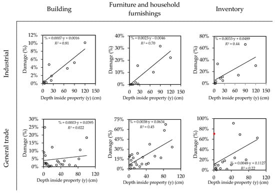
Figure 5.
Relationship of water depth inside the property and relative damage to building, furniture and household furnishings, and inventory, for industrial and general trade property uses.
For the scatter plot of some types of properties and assets, some outliers were identified for which low water depths caused unexpectedly high damage values. Some explanations in this regard may be given: 1) the heterogeneity of construction elements, 2) different furniture quality and costs, 3) stowage conditions, and 4) the existence of cold stores. As an example, the red dot in Figure 5 (general trade and inventory) indicates that very high relative damage occurred to the inventory (i.e., 70%) of a general trade when the property was only flooded by 1 cm.
Overall, some other inconsistencies may be discussed:
- The general trade category includes a variety of trades. They range from those that are more flood-resilient, such as outlets established in an industrial warehouse, to those more vulnerable to floods, such as fashion boutiques with parquet floors, cladding, and wood furniture.
- Damage to the inventory of chilled food trade occurs in a cascade. When cold stores are flooded with even a low floodwater depth, the damage could be total. However, in the case of a trade of construction materials, even when part of the inventory is flooded, it is possible to salvage the inventory placed on upper floors.
Particularly in terms of building assets, the linear correlations present an accurate fit in some cases but not in others, highlighting that, overall, the phenomenon is not well explained for low depths. It has been observed that for buildings from the majority of property types, the maximum relative damage is reached at 180 cm of water depth. This is the depth fixed for all buildings to reach maximum damage.
3.3.3. Depth‒Damage Curves’ Development for Barcelona
Based on the analysis of the available data and applying corrections according to the expert opinion, nationwide relative depth‒damage curves are initially developed. As stated by Van Vloten [55], in situations where there are no previous damage data or when the elements at risk are not comparable, consulting expert opinions on the matter is a good choice. This involves asking their opinion on the percentage of damage they expect for each structural type and for each hazard intensity. Expert opinions are also sought in the U.S. HAZUS methodology for the assessment of the impacts of flooding, for which depth‒damage functions were derived from expert opinion and historical data [56], as has been done in the present study. The report of the Gulf Engineers & Consultants (GEC) [51], developed for the USACE, explicitly highlighted the importance of insurance experts as a primary source for obtaining depth‒damage relationships. Also, in the work done by Bedford et al. [57], a variety of depth‒damage curves were proposed based on expert opinions and damage claims in 1993 and 1995.
To make the depth‒damage curves applicable to a specific municipality (i.e., Barcelona), these must be monetized by converting relative damage into economic damage per square meter (€/m2). In order to do this, the economic level of the target city is included. We must stress the importance of monetizing the curves of each type of asset separately and aggregating them afterwards into a single curve per type of property. In doing so, the disparity of prices for each type of asset in different municipalities may be taken into account. For instance, the cost of a building could be the same between two different municipalities, while the furniture, household furnishings, and inventory prices could be significantly different.
3.3.4. Regional Transferability to Other Spanish Urban Areas
Departing from the semi-empirical depth‒damage curves developed for Barcelona in the project RESCCUE, the present research goes further, proposing a methodology to transfer them to other Spanish municipalities. This allows for the use of depth‒damage curves for flood damage assessments at a national level through curves obtained under a standard methodology.
The regional transfer of Barcelona’s curves to a large number of the 8131 Spanish municipalities considers demographic, economic, and geographical factors, as they substantially influence the prices of goods and services across the country [16]. Regional adjustment indices have been obtained, taking as a reference Barcelona, based on indicators that are used as proxies of the expected regional price variability for the different assets’ curves (Figure 10). The original 14 types of property uses were grouped into three general sectors: commercial, industrial, and residential and others. These have been classified by type of asset in order to obtain three indicators (i.e., building, furniture and household furnishings, and inventory) (Table 5). For instance, the prices of buildings used as warehouses are assumed to vary, as commercial buildings do, but warehouses’ furniture, household furnishings, and inventory are more closely related to the price variability of the industrial sector. Relevant economic or market data at the municipal level are scarce, which was a limiting factor when developing the curves. Thus, when necessary, assumptions were made regarding the price or value variability of similar structures within a municipality.
Table 5.
Relationship between property uses and general sectors for assets.
Buildings, for the residential and others sector, represent the physical structure of the living space and the indicator selected to define their relative value per municipality is the average tax value per square meter for all properties’ transactions during the reference year 2020. These were obtained from an online real estate agent (www.idealista.com). For municipalities with no data available, the lowest value of their corresponding autonomous region has been considered as a proxy of the value, as those not represented are small, low-income towns. The baseline assumption is that the differences at a municipal level of the costs of damage reconstruction are comparable to the differences in property value. Continuing with the residential and others sector, the cost of damage to furniture and household furnishings is assumed to be aligned with the average disposable income per municipality. Hence, the indicator to compute the variation in content damage curves for the residential sector among municipalities is obtained through the statistics published by three sources: 1) the National Tax Agency (www.agenciatributaria.es), 2) the regional tax agency of the Basque Country (www.eustat.eus), and 3) the statistics agency of Navarra (www.navarra.es). Data were limited by the information provided by tax agencies that display small municipalities’ results in groups; thus, it was not possible to include municipalities with under 3000 inhabitants.
The residential and others sector does not consider inventory. Not all types of property uses include all three asset types. For instance, while car parks only consider building assets, offices contain the three types of assets.
Regarding the commercial and industrial sectors, the price variability among municipalities of the furniture (there are no household furnishings related to these sectors) and inventory has been explained through two indicators (n = 2): a) average revenues of each of the two sectors at the autonomous region scale, and b) the number of businesses per sector at a municipality level. The Sauerbeck index [58] (Equation (1)) was applied, defined as the arithmetic average of two or more reference prices to the rest of the municipalities’ relative values, on the basis of Barcelona prices. This was found to be the most appropriate way to introduce two related datasets that were at different geographical scales.
where n is the number of indicators (n = 2), s is the sector represented (i.e., commercial or industrial), mἰ denotes municipality i, and m0 is the reference municipality (i.e., Barcelona); AVs,mi represents the average economic value for the sectors of the autonomous region municipality i belongs to; NCs,mi stands for the number of companies of sector s registered in municipality i; and AVs,m0 and NCs,m0 represent the same values for the reference city of Barcelona.
In the furniture and household furnishings asset category, the variable AV takes the average investments in tangible assets per autonomous region for all companies registered under commercial and services sectors on the one hand, and the industrial sector on the other hand. For the inventory, the variable AV considers the average business revenue per autonomous region and sector. The number of commercial (commercial and services registered companies) and industrial companies per municipality (NC) comes from the national statistics office (www.ine.es). The lack of economic data at a local scale was an obstacle to including more precise values, and the two datasets alone do not provide any relevant measure. However, when combined they provide the local average revenue of the businesses belonging to each of the sectors displayed.
In summary, the spatial variability of the damage costs for the furniture and household furnishings can be explained by the differences in the average investment in tangible assets per municipality. In this sense, a city where the average investment to improve their assets is higher than the reference city (i.e., Barcelona), the damage caused to its business would be higher. The average local revenues are proposed to explain the inventory costs’ variability. This follows the rationale that, the higher the revenue in a municipality, the higher the inventory would be stocked in local businesses. Hence, the damage would be higher in the case of a flooding event. The spatial costs variability for buildings was established based on the property values for commercial, industrial, and residential sectors. The lack of data at a municipal level of commercial and industrial property values limited the range of action. However, the official property values (€/m2) of the three sectors from the Spanish Registrar Chartered Institute (www.registradores.org) were used to obtain the value variation at the autonomous regional level, which was then applied to the municipal property values. The final regional adjustment indices (RI) are obtained as decimal fractions referring to Barcelona (i.e., the unit).
3.3.5. Temporal Transferability
Regarding the price variability over time, a method to transfer damage curves to the future has been applied to the original depth‒damage curves developed for the year 2020 in Barcelona. The time horizon has been set to 2060, defined by the availability of the economic forecast. Long-term economic forecasting is a projection based on an assessment of the economic climate in individual countries and the world economy using both econometric models outputs and expert judgement [59]. Therefore, they can be characterized by uncertainty and complexity [60]. Considering this, and the scarcity of long-term projections, a temporal indicator has been developed using the OECD real GDP long-term forecast for Spain [61]. This is the most reliable source of information of its kind. Using the year 2020 as a reference, an indicator of the potential economic growth has been included up to 2060 in order to transfer present damage costs to future estimates. The final temporal adjustment indices (TI) are obtained as decimal fractions referring to 2020. Consequently, in order to obtain the depth‒damage curve of a certain municipality for a specific year, the total adjustment index (TAI) (Equation (2)) will be applied to each monetized asset curve of Barcelona (Table 7 and Figure 12):
where TAI is the total adjustment index, RI is the regional index, and TI is the temporal index.
Figure 6 presents the expected economic trend until 2060, thus the current depth‒damage curves can be updated accordingly by multiplying the monetized aggregated curves (i.e., including building and contents) by the temporal index for a specific year obtained through this function.
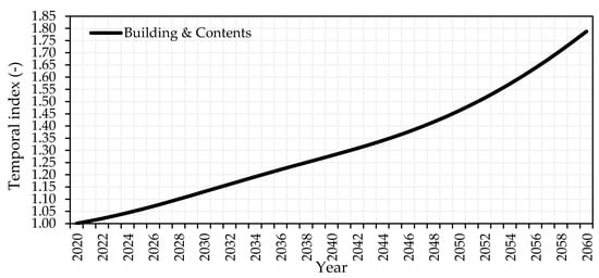
Figure 6.
Temporal adjustment indices to transfer present damage costs to future estimates for buildings and contents until the year 2060. Values based on the OECD real GDP long-term forecast for Spain [61].
3.3.6. Graphical Overview of the Proposed Methodology
Figure 7 gives an overview of the research process. It summarizes the key steps in the development of nationwide depth‒damage curves.
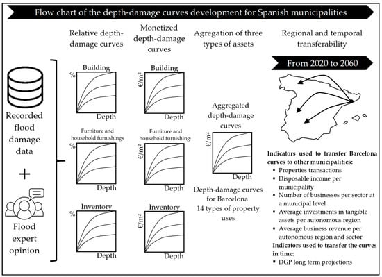
Figure 7.
Flowchart of the development of depth‒damage curves for Spanish municipalities.
4. Results
4.1. Relative Depth‒Damage Curves Development
The relative damage corresponding to intermediate water depths (between 10 cm and 180 cm), when the coefficient of determination is acceptable, has been set as the range for the linear regression. Nevertheless, relative damage for low depths (<10 cm) has been adapted according to the opinion of the flood expert surveyor. Regarding the damage related to high water depths (>180 cm), the maximum value has been set. Therefore, only in those situations where the correlation was not accurate enough has the curve been adjusted according to expert opinion. Figure 8a showcases an example of a relative depth‒damage curve proposed for the building of an industrial property. Inventory for commercial uses, though, except for those elements that require cold stores, tends to be at the same height, and accordingly its damage is also evenly distributed, as shown in Figure 8b. For the inventory, a maximum 100% relative damage has been considered, assuming that those elements that can be saved after flooding (e.g., plastic, construction materials, etc.) are not representative.
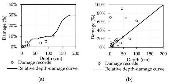
Figure 8.
Proposed relative depth‒damage curves and actual damage recorded for type of asset and property: (a) industrial buildings and (b) inventory, general trade.
Overall, the best correlations (linear) (i.e., high R2) were found for furniture and household furnishings, with values of R2 = 0.74 for restaurants and R2 = 0.82 for workshops. In these cases, damage related to low depths was set according to the expert opinion, and the maximum damage was set between 90% and 97% according to the type of property. Figure 9 shows, as an example, the relative depth‒damage curves proposed for furniture and household furnishings in restaurants and workshops.
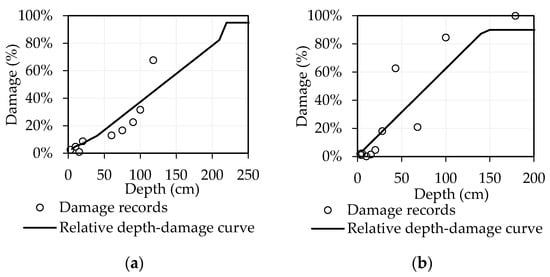
Figure 9.
Proposed relative depth‒damage curves and actual damage recorded for furniture and household furnishings and type of property: (a) restaurants and (b) workshops.
Figure 10 shows the proposed relative depth‒damage curves for each asset, building, furniture and household furnishings, and inventory, according to 14 different types of property uses. These semi-empirical curves are developed to be applied in any Spanish municipality. Therefore, the curves’ shape are invariable in both space (in Spain) and time.
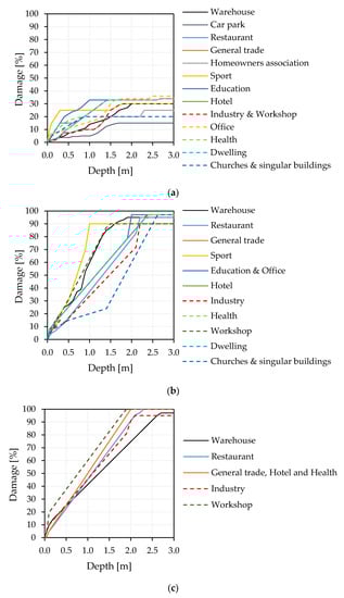
Figure 10.
Relative depth‒damage curves for Spanish cities: (a) buildings, (b) furniture and household furnishings, and (c) inventory.
4.2. Monetization of Relative Damage for Barcelona
To monetize the curves for Barcelona, initially the deciles (cost(€)/m2) from the distribution of the data sample for each type of property and asset have been determined. According to expert opinion, a specific decile has been established for each type of property based on the target city. In some cases, the expert suggested providing an average value or making a direct estimation when the deciles did not match with his criterion, as Table 6 presents.
Table 6.
Proposed cost (€/m2) for assets (i.e., building, furniture and household furnishings, and inventory) for each type of property in Barcelona.
Once an adequate cost per square meter was associated with each property and asset according to the expert opinion for Barcelona, depth‒damage curves were constructed for each asset. The following aggregation of the three types of assets provided the total depth‒damage curves (Figure 11).
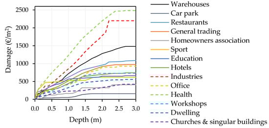
Figure 11.
Semi-empirical depth‒damage curves for Barcelona.
For those type of properties and assets with data scarcity or those that presented a low coefficient of determination, the expert used his criterion to adjust a curve from other property uses expected to be similar.
4.3. Depth‒Damage Curves for Other Spanish Municipalities
As an example, Table 7 presents the regional indexes (RI) corresponding to some of the most damaged municipalities in Spain (Figure A1) due to flooding, which allows for constructing their own depth‒damage curves (Figure 12).
Table 7.
Regional indexes by assets in general use for the 10 most damaged municipalities in Spain, 1995–2019.
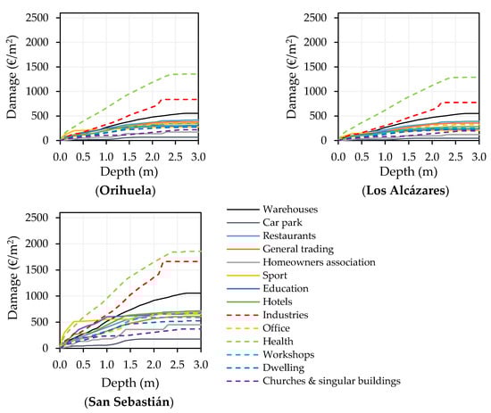
Figure 12.
Depth‒damage curves for some of the most damaged municipalities in Spain due to flooding (pluvial and fluvial) for the 2020 reference year.
The literature is scarce on the spatial transferability of damage curves, but a similar study by the IBI Group for Alberta (Canada) [16] uses the results of a local consumer price index survey to transfer damage to all economic sectors. Therefore, although limitations still exist, the present study represents an improvement on the current state of the field.
5. Conclusions
The use of depth‒damage curves is globally accepted, even acknowledging the omission of other relevant variables, such as the water velocity or the floodwater residence time. A number of flood damage models are based on the use of these water‒damage relationships. One of their major limitations is their site-specific nature, which means they cannot be applied in other regions. Moreover, the need of price updating may be considered a limitation, too. These issues are discussed in the literature and there is broad agreement about the better performance of relative depth‒damage functions that remain static at least in time. Their shape, though, in terms of regional transferability, is more dependent on the style and typology of construction, which could be assumed to be fairly uniform at a national level. Maybe, for these reasons, standardizing a methodology of curves at a European level does not seem feasible yet, as some authors indicate discrepancies among computed and actual damage when using these continent-wide curves. Besides, countries such as the United Kingdom (Multi Colour Manual) and the United States of America (HAZUS-MH) apply their own nationwide depth‒damage curves, and they have been well accepted for many years.
Barcelona is one of the case studies of the EU-funded RESCCUE project, whereby a comprehensive analysis of its climate resilience has been carried out. The impact of increasingly frequent pluvial floods has been analyzed. Namely, a detailed flood damage assessment has been conducted for the entire city, focusing primarily on properties. Due to the lack of existing detailed depth‒damage curves for Barcelona, a tailored approach has been used, considering the 14 types of properties commonly found in highly urbanized cities. These developments were based on a sample of actual damage records; when insufficient or when the correlation between the damage and water depth was poor, the contribution of a flood expert surveyor was essential. Therefore, as in many other previous studies, expert opinion was included, resulting in the construction of semi-empirical depth‒damage curves for Barcelona. In addition, this paper offers a methodology to obtain the depth‒damage curves for any Spanish municipality, which provides standardization of depth‒damage curves at a national level.
The methodology to standardize the construction of depth‒damage curves in Spain presented here will contribute to enhancing cost‒benefit studies in flood damage assessments at a micro scale and will allow for the comparison of results between different regions of the country. This could take on special relevance for future reviews and updates of flood risk management plans in Spain in the framework of the European Directive 2007/60/CE, included in the Spanish legislation through the Royal Decree 903/2010.
Author Contributions
Conceptualization, E.M.-G. and M.G.-H.; methodology, E.M.-G., M.G.-H., E.F.-O. and S.C.; validation, E.M.-G. and M.G.; formal analysis, E.M.-G.; investigation, E.M.-G., E.F.-O. and M.G.-H.; resources, S.C.; data curation, S.C. and E.M.-G.; writing—original draft preparation, E.M.-G.; writing—review and editing, M.G.; visualization, E.M.-G.; supervision, M.G.; project administration, E.M.-G.; funding acquisition, E.M.-G. and M.G.-H. All authors have read and agreed to the published version of the manuscript.
Funding
This research was funded by Horizon 2020 Framework Programme, Grant Agreement No. 700174.
Acknowledgments
The authors thank the Spanish insurance company Consorcio de Compensación de Seguros (CCS) for its important role in this research. Without its collaboration by providing claims data the damage model would have not been calibrated properly.
Conflicts of Interest
The authors declare no conflict of interest.
Appendix A
Figure A1 indicates the 20 municipalities in Spain most damaged by flooding in 1995–2019, which considers both pluvial and fluvial floods, but only damage to properties. The values indicated in the graph correspond to the compensation paid by the CCS.

Figure A1.
The 20 most damaged municipalities in Spain due to flooding (pluvial and fluvial) according to the compensations paid by the CCS.
Figure A1.
The 20 most damaged municipalities in Spain due to flooding (pluvial and fluvial) according to the compensations paid by the CCS.

References
- European Environment Agency. Economic Losses from Climate-Related Extremes in Europe; Copenhagen, Denmark, 2019; p. 28. Available online: https://www.eea.europa.eu/data-and-maps/indicators/direct-losses-from-weather-disasters-3/assessment-2 (accessed on 20 January 2020).
- Improving Damage Assessments to Enhance Cost-Benefit Analyses (IDEA) Project Earthquake of Lorca in 2011. Available online: http://www.ideaproject.polimi.it/?portfolio=floods-in-vall-daran-and-pyrenees (accessed on 22 February 2020).
- United Nations, Department of Economic and Social Affairs, Population Division. World Urbanization Prospects: The 2018 Revision (ST/ESA/SER.A/420); New York, NY, USA, 2018; p. 126. Available online: https://population.un.org/wup/Publications/Files/WUP2018-Report.pdf (accessed on 20 January 2020).
- European Environmental Agency (EEA). Flood Risk in Europe: the Long-Term Outlook; European Environmental Agency (EEA): Copenhague, Denmark, 2016. [Google Scholar]
- Velasco, M.; Cabello, À.; Russo, B. Flood damage assessment in urban areas. Application to the Raval district of Barcelona using synthetic depth damage curves. Urban Water J. 2016, 13, 426–440. [Google Scholar] [CrossRef]
- White, G.F. Human Adjustment to Floods: A Geographical Approach to the Flood Problem in the United States. Ph.D. Dissertation, University of Chicago, Chicago, MA, USA, 1945. [Google Scholar]
- Manrique, A.; Nájera, A.; Escartín, C.; Moreno, C.; Martínez, E.; Espejo, F.; Sánchez, F.J.; Aparicio, M.; Cordero, S.; González, S. Guía Para la Reducción de la Vulnerabilidad de Los Edificios Frente a Las Inundaciones. Consorcio de Compensación de Seguros (CCS); Madrid, Spain, 2017; p. 106. Available online: https://www.consorseguros.es/web/documents/10184/48069/guia_inundaciones_completa_22jun.pdf (accessed on 14 March 2018).
- The European Parliament and the Council of the European Union Directive 2007/60/EC of the European Parliament and of the Council of 23 October 2007 on the Assessment and Management of Flood Risks (Text with EEA Relevance). 2007, p. 8. Available online: https://eur-lex.europa.eu/legal-content/EN/TXT/PDF/?uri=CELEX:32007L0060&from=EN (accessed on 11 February 2020).
- Ministerio de la Presidencia Real Decreto 903/2010, de 9 de julio, de evaluación y gestión de riesgos de inundación. 2010, p. 14. Available online: https://www.boe.es/buscar/doc.php?id=BOE-A-2010-11184. (accessed on 11 February 2020).
- Arnbjerg-Nielsen, K.; Willems, P.; Olsson, J.; Beecham, S.; Pathirana, A.; Bülow Gregersen, I.; Madsen, H.; Nguyen, V.-T.-V. Impacts of climate change on rainfall extremes and urban drainage systems: A review. Water Sci. Technol. 2013, 68, 16–28. [Google Scholar] [CrossRef] [PubMed]
- Nafari, R.H.; Ngo, T. Predictive applications of australian flood loss models after a temporal and spatial transfer. Geomat. Nat. Hazards Risk 2018, 9, 416–430. [Google Scholar] [CrossRef]
- Amadio, M.; Rita Scorzini, A.; Carisi, F.; Essenfelder, H.A.; Domeneghetti, A.; Mysiak, J.; Castellarin, A. Testing empirical and synthetic flood damage models: The case of Italy. Nat. Hazards Earth Syst. Sci. 2019, 19, 661–678. [Google Scholar] [CrossRef]
- Federal Emergency Management Agency (FEMA). Department of Homeland Security. Mitigation Division Multi-hazard Loss Estimation Methodology. Flood Model. Hazus-HM MR5 Technical Manual; Federal Emergency Management Agency (FEMA): Washington, DC, USA, 2015; Volume 499. [Google Scholar]
- U.S. Army Corps of Engineers (USACE). HEC-FDA User’s Manual. Flood Damage Reduction Analysis; U.S. Army Corps of Engineers (USACE): Washington, DC, USA, 2016; p. 392.
- Jongman, B.; Kreibich, H.; Apel, H.; Barredo, J.I.; Bates, P.D.; Feyen, L.; Gericke, A.; Neal, J.; Aerts, J.C.J.H.; Ward, P.J. Comparative flood damage model assessment: Towards a European approach. Nat. Hazards Earth Syst. Sci. 2012, 12, 3733–3752. [Google Scholar] [CrossRef]
- IBI Group. Provincial Flood Damage Assessment Study. Prepared for Government of Alberta; IBI Group: Calgary, AB, Canada, 2015. [Google Scholar]
- Carisi, F.; Schröter, K.; Domeneghetti, A.; Kreibich, H.; Castellarin, A. Development and assessment of uni- and multivariable flood loss models for Emilia-Romagna (Italy). Nat. Hazards Earth Syst. Sci. 2018, 18, 2057–2079. [Google Scholar] [CrossRef]
- U.S. Army Corps of Engineers (USACE). Economic Guidance Memorandum (EGM) 04-01, Generic Depth-Damage Relationships for Residential Structures with Basements; U.S. Army Corps of Engineers (USACE): Washington, DC, USA, 2003.
- Jan, H.; Hans, D.M.; Wojciech, S. Global Flood Depth-Damage Functions: Methodology and the Database with Guidelines | EU Science Hub; Joint Research Centre: Ispra, Italy, 2017. [Google Scholar]
- Nafari, R.H.; Ngo, T.; Mendis, P. An assessment of the effectiveness of tree-based models for multi-variate flood damage assessment in Australia. Water 2016, 8, 282. [Google Scholar] [CrossRef]
- Hasanzadeh Nafari, R.; Ngo, T.; Lehman, W. Development and evaluation of FLFAcs—A new Flood Loss Function for Australian commercial structures. Int. J. Disaster Risk Reduct. 2016, 17, 13–23. [Google Scholar] [CrossRef]
- Hasanzadeh Nafari, R.; Ngo, T.; Lehman, W. Calibration and validation of FLFArs-A new flood loss function for Australian residential structures. Nat. Hazards Earth Syst. Sci. 2016, 16, 15–27. [Google Scholar] [CrossRef]
- Olesen, L.; Löwe, R.; Arnbjerg-Nielsen, K. Flood Damage Assessment Literature Review and Recommended Procedure; Cooperative Research Centre for Water Sensitive Cities: Melbourne, Australia, 2017; Volume 4, ISBN 9781921912399. [Google Scholar]
- Vanneuville, W.; Maddens, R.; Collard, C.; Bogaert, P.; De Maeyer, P.; Antrop, M. Impact op mens en economie t.g.v. overstromingen bekeken in het licht van wijzigende hydraulische condities, omgevingsfactoren en klimatologische omstandigheden 2006, 2.
- McGrath, H.; Abo El Ezz, A.; Nastev, M. Probabilistic depth–damage curves for assessment of flood-induced building losses. Nat. Hazards 2019, 97, 1–14. [Google Scholar] [CrossRef]
- Cammerer, H.; Thieken, A.H.; Lammel, J. Adaptability and transferability of flood loss functions in residential areas. Nat. Hazards Earth Syst. Sci. 2013, 13, 3063–3081. [Google Scholar] [CrossRef]
- Hasanzadeh Nafari, R.; Amadio, M.; Ngo, T.; Mysiak, J.; Nafari, R.H.; Amadio, M.; Ngo, T.; Mysiak, J. Flood loss modelling with FLF-IT: A new flood loss function for Italian residential structures. Nat. Hazards Earth Syst. Sci. 2017, 17, 1047–1059. [Google Scholar] [CrossRef]
- Reese, S.; Ramsay, D. RiskScape: Flood fragility methodology. Technical Report: WLG2010-45; New Zealand Climate Change Research Institute, Victoria University of Wellington: Kilbirnie, New Zealand; Wellington, New Zealand, 2010. [Google Scholar]
- Huizinga, H.J.; Dijkman, M.; Barendregt, A.; Waterman, R. HIS - Schade en Slachtoffer Module Versie 2.1; Ministry of Transport and Water Management: The Hague, The Netherlands, 2005. [Google Scholar]
- Milieu- en Natuurplanbureau (MNP). Delft Hydraulics Overstromingsrisico’s in Nederland in een Veranderend Klimaat; Milieu- en Natuurplanbureau (MNP): Delft, The Netherlands, 2007. [Google Scholar]
- Penning-Rowsell, E.; Viavattene, C.; Parode, J.; Chatterton, J.; Parker, D.; Morris, J. The Benefits of Flood and Coastal Risk Management: A Handbook of Assessment Techniques-2010 (Multi-Coloured Manual); book+ CD-ROM with damage data; FHRC: London, UK, 2010. [Google Scholar]
- Federal Emergency Management Agency (FEMA). Hazus Flood Model User Guidance; Federal Emergency Management Agency (FEMA): Washington, DC, USA, 2018.
- Karamouz, M.; Fereshtehpour, M.; Ahmadvand, F.; Zahmatkesh, Z. Coastal flood damage estimator: An alternative to FEMA’s HAZUS platform. J. Irrig. Drain. Eng. 2016, 142, 1–12. [Google Scholar] [CrossRef]
- Cutrell, A.K.; Rozelle, J.; Hines, S.H. FEMA Standard Operating Procedure for Hazus Flood Level 2 Analysis Hazus Flood Model; Federal Emergency Management Agency (FEMA): Washington, DC, USA, 2018.
- Huizinga, J.; De Moel, H.; Szewczyk, W. Global Flood Depth-Damage Functions: Methodology and the Database with Guidelines; Joint Research Centre: Sevilla, Spain, 2017. [Google Scholar]
- Luino, F.; Cirio, C.G.; Biddoccu, M.; Agangi, A.; Giulietto, W.; Godone, F.; Nigrelli, G. Application of a model to the evaluation of flood damage. Geoinformatica 2009, 13, 339–353. [Google Scholar] [CrossRef]
- Freni, G.; La Loggia, G.; Notaro, V. Uncertainty in urban flood damage assessment due to urban drainage modelling and depth-damage curve estimation. Water Sci. Technol. 2010, 61, 2979–2993. [Google Scholar] [CrossRef]
- Pistrika, A.; Tsakiris, G.; Nalbantis, I. Flood depth-damage functions for built environment. Environ. Process. 2014, 1, 553–572. [Google Scholar] [CrossRef]
- Tariq, M.A.U.R.; Hoes, O.A.C.; Van de Giesen, N.C. Development of a risk-based framework to integrate flood insurance. J. Flood Risk Manag. 2014, 7, 291–307. [Google Scholar] [CrossRef]
- Budiyono, Y.; Aerts, J.; Brinkman, J.J.; Marfai, M.A.; Ward, P. Flood risk assessment for delta mega-cities: A case study of Jakarta. Nat. Hazards 2015, 75, 389–413. [Google Scholar] [CrossRef]
- Central Intelligence Agency The World Factbook. Available online: https://www.cia.gov/library/publications/resources/the-world-factbook/index.html (accessed on 11 February 2020).
- Aerts, J.C.J.H.; Botzen, W.J.W. Climate adaptation cost for flood risk management in the Netherlands. In Proceedings of the conference Storm Surge Barriers to Protect New York City Against The Deluge, Brooklyn, NY, USA, 30–31 March 2009; pp. 99–113. [Google Scholar]
- Bussi, G.; Ortiz, E.; Francés, F.; Pujol, L.; De Ingeniería, I.; De València, U.P.; De Vera, C.; Hidrográfica, C.; Ibañez, A.B.; Bellver, P.; et al. Modelación hidráulica y análisis del riesgo de inundación según las líneas guía de la Directiva Marco del Agua. El caso de la Marina Alta y la Marina Baja (Alicante). II Jornadas sobre Ing. del Agua. 2007, 10. Available online: http://lluvia.dihma.upv.es/es/publi/congres/050_JIA2011_PRESENTACION_GB_articulo.pdf (accessed on 10 January 2020).
- Ministry of Agriculture, Fisheries and Food (MAGRAMA). Propuesta de Mínimos Para la Metodología de Realización de los Mapas de Riesgo de Inundación; Ministry of Agriculture, Fisheries and Food (MAGRAMA): Madrid, Spain, 2013. [Google Scholar]
- Valenciana, C. Plan de Acción Sobre Prevención del Riesgo de Inundación en la Comunitat Valenciana (PATRICOVA); Generalitat Valenciana: Valencia, Spain, 2015. [Google Scholar]
- Demarcación Hidrográfica del Cantábrico Oriental. Plan de Gestión del Riesgo de Inundación 2015-2021; Demarcación Hidrográfica del Cantábrico Oriental: San Sebastián, Spain, 2016. [Google Scholar]
- Ritter, J.; Berenguer, M.; Corral, C.; Park, S.; Sempere-Torres, D. ReAFFIRM: Real-time Assessment of Flash Flood Impacts – a Regional high-resolution Method. Environ. Int. 2020, 136, 105375. [Google Scholar] [CrossRef]
- Van Ootegem, L.; Van Herck, K.; Creten, T.; Verhofstadt, E.; Foresti, L.; Goudenhoofdt, E.; Reyniers, M.; Delobbe, L.; Murla Tuyls, D.; Willems, P. Exploring the potential of multivariate depth-damage and rainfall-damage models. J. Flood Risk Manag. 2018, 11, S916–S929. [Google Scholar] [CrossRef]
- Wagenaar, D.; Lüdtke, S.; Schröter, K.; Bouwer, L.M.; Kreibich, H. Regional and temporal transferability of multivariable flood damage models. Water Resour. Res. 2018, 54, 3688–3703. [Google Scholar] [CrossRef]
- Jamali, B.; Löwe, R.; Bach, P.M.; Urich, C.; Arnbjerg-Nielsen, K.; Deletic, A. A rapid urban flood inundation and damage assessment model. J. Hydrol. 2018, 564, 1085–1098. [Google Scholar] [CrossRef]
- Gulf Engineers & Consultants (GEC). Depth-Damage Relationships for Structures, Contents, and Vehicles and Content-to-Structure Value Ratios (CSVR) in Support of the Donaldsonville to the Gulf, Luisiana, Feasibility Study; Gulf Engineers & Consultants (GEC): New Orleans, LA, USA, 2006. [Google Scholar]
- Mitchell, A.; Dodge, B.; Kruzic, P.; Miller, D.; Schwartz, P. Handbook of Forecasting Techniques; National Technical Information Service U. S. Department of Commerce: Springfield, VA, USA, 1975.
- Mitchell, A.; Dodge, B.H. Handbook of Forecasting Techniques. Part 2. Description of 31 Techniques; National Technical Information Service U. S. Department of Commerce: Springfield, VA, USA, 1977.
- Boletín Económico de la Construcción (BEC) Revista de Información Económica (Precios Unitarios y Descompuestos) Dirigida a Profesionales del Sector de la Construcción. No 309. Available online: https://becsl.es (accessed on 1 July 2019).
- Van Vloten, S.O. Vulnerability and Flood Risk in Urban Areas. Bachelor’s Thesis, Universitat Politècnica de Catalunya, Barcelona, Spain, 2014. [Google Scholar]
- Scawthorn, C.; Flores, P.; Blais, N.; Seligson, H.; Tate, E.; Chang, S.; Mifflin, E.; Thomas, W.; Murphy, J.; Jones, C.; et al. HAZUS-MH flood loss estimation methodology. II. Damage and loss assessment. Nat. Hazards Rev. 2006, 7, 72–81. [Google Scholar] [CrossRef]
- Bedford, T.; van Gelder, P.; Guedes Soares, C.; van Manen, S.E.; Brinkhuis, M. Quantitative flood risk assessment for Polders. Reliab. Eng. Syst. Saf. 2005, 90, 229–237. [Google Scholar]
- Statistical Office of the European Communities. Export and Import Price Index Manual: Theory and Practice; International Monetary Fund: Washington, DC, USA, 2009; ISBN 9264085416. [Google Scholar]
- OECD “Long-term baseline projections, No. 103”, OECD. Econ. Outlook Stat. Proj. 2020. Available online: https://doi:10.1787/68465614-en (accessed on 18 February 2020).
- D’Amico, S.; Orphanides, A. Uncertainty and Disagreement in Economic Forecasting; Finance and Economics Discussion Series; Divisions of Research & Statistics and Monetary Affairs, Federal Reserve Board: Washington, DC, USA, 2008. [Google Scholar]
- OECD Real GDP Long-Term Forecast (Indicator). Available online: https://doi.org/10.1787/d927bc18-en (accessed on 18 February 2020).


© 2020 by the authors. Licensee MDPI, Basel, Switzerland. This article is an open access article distributed under the terms and conditions of the Creative Commons Attribution (CC BY) license (http://creativecommons.org/licenses/by/4.0/).