Abstract
Air pollution is a common problem for many countries around the world in the process of industrialization as well as a challenge to sustainable development. This paper has selected Chengdu-Chongqing region of China as the research object, which suffers from severe air pollution and has been actively involved in air pollution control in recent years to achieve sustainable development. Based on the historical data of 16 cities in this region from January 2015 to November 2019 on six major air pollutants, this paper has first conducted evaluation on the monthly air quality of these cities within the research period by using Principal Component Analysis and the Technique for Order Preference by Similarity to an Ideal Solution. Based on that, this paper has adopted the Long Short-Term Memory neural network model in deep learning to forecast the monthly air quality of various cities from December 2019 to November 2020. The aims of this paper are to enrich existing literature on air pollution control, and provide a novel scientific tool for design and formulation of air pollution control policies by innovatively integrating commonly used evaluation models and deep learning forecast methods. According to the research results, in terms of historical evaluation, the air quality of cities in the Chengdu-Chongqing region was generally moving in the same trend in the research period, with distinct characteristics of cyclicity and convergence. Year- on-year speaking, the effectiveness of air pollution control in various cities has shown a visible improvement trend. For example, Ya’an’s lowest air quality evaluation score has improved from 0.3494 in 2015 to 0.4504 in 2019; Zigong’s lowest air quality score has also risen from 0.4160 in 2015 to 0.6429 in 2019. Based on the above historical evaluation and deep learning forecast results, this paper has proposed relevant policy recommendations for air pollution control in the Chengdu-Chongqing region.
1. Introduction
In the process of economic development, the improvement in industrial production capacity plays a decisive role, and it is often the only way for a country to achieve modernization [1,2,3]. However, according to historical experience, with the progression of economic development, air pollution brought by industrial production will usually become an important obstacle to the sustainable development [4,5,6].
As one of the major developing countries, China is facing increasingly prominent air pollution problems after over 40 years of rapid economic growth [7,8,9]. Air pollution control and protection of sustainable development has become a priority of the government [10,11]. Since 2010, China’s central government and local governments at all levels have attached great importance to air pollution control [12,13,14]. China’s top leadership has put forward the philosophy of “green hills and clear waters are as precious as gold and silver” [15], and included pollution control and ecological civilization in the constitution of China [16]. Therefore, behind all these political slogans and mobilization, the actual effectiveness of China’s air pollution control campaigns in recent years has become an important topic of general concern to the academia [17,18,19,20].
However, the existing academic research on China’s air pollution and pollution control often focus on the Beijing-Tianjin-Hebei, Yangtze River Delta, and Pearl River Delta regions, but pay relatively less attention to the Chengdu-Chongqing region located in Midwest China. For example, Li et al. [21] established a multi-regional computable general equilibrium model to evaluate the impact of China’s air pollution abatement policies in the Beijing-Tianjin-Hebei area. They have shown that those policies would cause an average loss of 1.4% of Gross Regional Product growth every year. Among those policies, the end-of-pipe control has been identified as the most efficient one for air pollutant reduction. Xiao et al. [22] have used the air quality data collected from 161 air monitoring stations in Beijing-Tianjin-Hebei region to construct the indicator system for urban air quality assessment. Their results showed that PM2.5, PM10 and SO2 improved from 2015 to 2018, while ozone deteriorated significantly. Further, they used the multiple linear regression model to reveal the negative correlation between air quality and meteorological factors. Yun et al. [23] studied the spatial distribution and variation characteristics of PM2.5 and its influencing factors in the Yangtze River Delta from 2005 to 2015. By remote sensing inversion of PM2.5 and spatial statistical analyses, they have found that the formation of PM2.5 is dominantly affected by CO2 emissions and population density, and PM2.5 concentration diffusion is mainly driven by regional climate and geomorphology. Bao et al. [24] collected real-time observation data of PM2.5, PM10, SO2, NO2, CO and O3 in the Yangtze River Delta region to analyze wintertime haze events. Constructing hybrid receptor models, they have identified source regions of PM2.5 and found that air pollution is significantly affected by local emissions and regional transportation. Wu et al. [25] have assessed the effectiveness of pollution control policies in the Pearl River Delta and estimated the trends of premature mortality attributable to PM2.5 and O3. They found that the PM2.5-related premature deaths varied little with respect to time, while the O3-related premature deaths increased significantly because of the increases in both O3 concentration and exposed population, especially in the central Pearl River Delta including Guangzhou, Foshan, Dongguan, and Shenzhen. Xie et al. [26] utilized the clustering technique to study the effect modulation of the clustered local wind fields have on air quality in the Pearl River Delta. They found the wind-dependent spatial characteristics of PM2.5, PM10, and NO2 concentrations.
Contrasted to existing literature, this paper has selected the Chengdu-Chongqing region as the research project for the following reasons:
- (1)
- Geographic Location.The Chengdu-Chongqing region is located in the Sichuan Basin in inland China. The landform of basin does not provide favorable natural conditions for the diffusion of air pollution compared to the coastal areas [27,28,29]. It is the general consensus in the academic community that climatic conditions are one of the most important constraints for air pollution control [30,31,32,33,34]. The precipitation in the Sichuan Basin is lower than that in the Yangtze River Delta and Pearl River Delta region in all seasons, and this region is a low-wind speed area with an average wind speed of below 1.5 m/s in all seasons, which is significantly lower than that in the Beijing-Tianjin-Hebei, Yangtze River Delta, and Pearl River Delta region [35]. Therefore, compared to the Yangtze River Delta and Pearl River Delta region, the air quality in Chengdu-Chongqing region can better reflect the actual effectiveness of air pollution control policies.
- (2)
- Economic Industries.Due to its location in central China, the economic development of the Chengdu-Chongqing region is relatively slower than that of the coastal areas [36,37,38]. Although Sichuan province has kept a GDP growth rate of over 10% from 2005 to 2013, its GDP growth has dropped significantly after 2014 [39]. Therefore, maintaining local economic growth while combating air pollution and shutting down heavily polluting enterprises is presenting more challenges to the local government. In addition, since 2010, the traditional industries in the Chengdu-Chongqing region have been experiencing weak growth and this region is looking for new pillar industries to achieve economic transformation [40,41,42].In view of this, this paper has collected the monthly average data of six major air pollutants of 16 cities in the Chengdu-Chongqing region (including 15 cities of Sichuan Province and Chongqing, the municipality directly under the central government) from January 2015 to November 2019. The paper first conducts evaluation of the air quality of various cities within the research period by using the Principal Component Analysis (PCA) and the Technique for Order Preference by Similarity to an Ideal Solution (TOPSIS) models. Based on that, the paper further utilizes the Long Short-Term Memory neural network model in deep learning to forecast the monthly air quality of each city from December 2019 to November 2020 in order to show the historical effectiveness and simulate future performance of the air pollution control policies of these cities.
Through the above research, this paper strives to achieve the following two aims:
- (1)
- Enrich existing literature on air pollution control by selecting the typical region of a large developing country as the research object, analyzing its air pollution control policies as well as the effectiveness in-depth, and making scientific forecast of the air quality in one year;
- (2)
- Provide a novel scientific tool for design and formulation of air pollution control policies by innovatively integrating commonly used evaluation models and deep learning forecast methods, fully utilizing historical data and applying innovative algorithms to the field of air pollution control.
In the existing literature, on the one hand, Multi-Criteria Decision Making (MCDM) methods are commonly used for air quality assessment. Based on the MCDM method, Chalabi et al. [43] combined the chemistry transport model and health impact model to assess the air quality policies in the United Kingdom. Their results show that, taking into account all standards, reducing industrial combustion emissions is the most valuable for improving air quality. Wang et al. [44] used MCDM method to evaluate the impact of air pollution on urban economic development. By proposing an improved Technique for Order of Preference by Similarity to Ideal Solution (TOPSIS) model, they evaluated various factors of air pollutants and economic development. Moreover, they optimized the model training process to overcome the traditional disadvantages of the TOPSIS method. Using the MCDM method, Caravaggio et al. [45] evaluated 10 air pollutants in 30 European countries from 2008 to 2015 from a macro perspective. By merging the relevant procedures commonly used in environmental assessment under the MCDM framework, they conducted cluster analysis based on the relative performance of air pollution in various countries, which provides a comprehensive picture of the European economy and discloses the advantages and disadvantages of controlling atmospheric pollutants in those countries. Chen et al. [46] used the MCDM method and the alternative method based on causality to analyze potential improvement strategies for air quality in Kaohsiung, Taiwan. By assessing the correlation between different air quality improvement standards and focusing on providing long-term improvements, they argued that coal-fired power plants and factory exhausts are the main source of pollution in Kaohsiung City, and environmental authorities should urge those factories to continuously improve energy efficiency to reduce pollutant emissions. Chauvy et al. [47] used the MCDM method to evaluate the use of carbon dioxide. They divided the evaluation indicators into three dimensions: engineering, economy and environment, and discussed the application of decision analysis methods. Their results show that in the process of making full use of carbon dioxide to reduce atmospheric pollution, that technical, economic and environmental aspects are complementary, but not interchangeable. At the same time, low-level compensation methods should be used to promote carbon dioxide emissions reduction.
On the other hand, neural networks are commonly used for air quality prediction. Alimissis et al. [48] used real data from the urban air quality monitoring network in Athens, Greece, with the help of artificial neural networks and multiple linear regression methods to predict the future spatial situation of nitrogen dioxide, nitric oxide, ozone, carbon monoxide and sulfur dioxide. They demonstrated that the spatial correlation between monitoring stations will be reduced under the condition of limited atmospheric quality network density. Therefore, the artificial neural network method has advantages in predicting atmospheric quality compared with the multiple linear regression method. Zhao et al. [49] built a Long Short-Term Memory (LSTM) fully connected neural network model, and used China’s historical air quality data to predict PM2.5 pollution data for specific air quality monitoring stations within 48 h. This neural network model was used to analyze the correlation between PM2.5 pollution at the central station and adjacent stations in Beijing from 1 May 2014 to 30 April 2015. Zhou et al. [50] established a Deep Multi-output LSTM neural network model, which combines mini-batch gradient descent algorithm, dropout neuron algorithm, and L2 regularization algorithm to analyze the key factors of complex spatiotemporal relationships. Through the analysis and prediction of data from five air quality monitoring stations in Taipei, Taiwan, they found that the proposed neural network model and algorithms can significantly improve the accuracy of regional multi-level air quality forecast. Maleki et al. [51] built an artificial neural network model to predict hourly standard air pollutant concentration, air quality index and air quality health index. By analyzing the air pollution data of Ahvaz, Iran, from August 2009 to August 2010, they obtained the model’s predicted correlation coefficient and root-mean square error of 0.87 and 59.9, respectively. The results show that artificial neural networks can be used to predict air quality and thus prevent health effects. Fong et al. [52] used Long Short-Term Memory (LSTM) recurrent neural networks to predict the future air pollutant concentration in Macau. The experimental sample spans more than 12 years and includes daily measurements from multiple air pollutants and other more classic meteorological values. Their results show that the neural networks have high prediction accuracy. It has a shorter training time than the randomly initialized recurrent neural network.
Based on the existing literatures, the PCA and TOPSIS method are combined to evaluate the historical air pollution situation in Chengdu-Chongqing Region, and the deep learning forecast for the future air pollution situation are conducted by the Long Short-Term Memory (LSTM) neural network model in this paper, which realizes research novelties compared to the existing literatures.
2. Materials and Methods
2.1. Research Objects and Data Sources
The 16 cities in the Chengdu-Chongqing region include: Chengdu, Chongqing, Dazhou, Deyang, Guang’an, Leshan, Luzhou, Meishan, Mianyang, Nanchong, Neijiang, Suining, Ya’an, Yibin, Zigong, and Ziyang. Among them, Chongqing is one of the four municipalities directly under the Central Government of China, and Chengdu is the provincial capital of Sichuan Province [36]. These two cities have the important status of “leaders” in the region (see Figure 1).
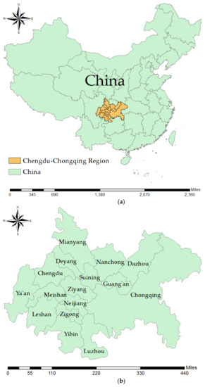
Figure 1.
Cities in Chengdu-Chongqing region: (a) Chengdu-Chongqing region in China; (b) Geographical locations of cities in Sichuan-Chongqing region [36].
The data used in this paper includes statistics on six major air pollutants in 16 cities, which are separated cities according to China’s official administrative divisions of the Chengdu-Chongqing region. The research period is from January 2015 to November 2019. Based on China’s national air quality standards, this paper has selected the monthly average concentration data of six major pollutants: PM2.5, PM10, CO, NO2, O3, and SO2 [53,54]. Then, the monthly average concentration data of six major pollutants were individually divided by the number of the population in each city (per million population) to obtain the concentration data of every pollutant corresponding to each million of people in that city during the period of research. The data sources include: China National Environmental Monitoring Center [55], Data Center of China’s Ministry of Environmental Protection [56], air quality and pollutant monitoring reports released by Sichuan Province [57], and the air quality and pollutant monitoring reports issued by Chongqing City [58]. It should be pointed out that regional grid monitoring will provide a good idea of where the pollution is and at what levels, but it is expensive to have so many monitors. Many places use hot-spot monitoring and locate measuring sites where specific worst-case situations exist. These systems over-estimate the regional levels and are resistant to showing improvements in some situations, while over-estimating improvements if the specific cause of the “hot-spot” has been eliminated. In order to avoid the impacts from those factors, this paper used those abovementioned official statistics, and the values of all pollutants have been comprehensively calculated based on the data collected from all monitoring locations in this city. As the air pollutant concentration data are reported on a daily basis (1795 days in all), this paper has calculated the monthly average concentration of various pollutants based on the daily statistics to form a data set for air quality evaluation and forecast.
Let the number of samples in this data set be , and the indicator value of the pollutant in the sample be . The definition of each variable is shown below in Table 1:

Table 1.
Definitions of variables.
When used to perform evaluation and forecast, these data need to be de-averaged and normalized to arrive at a standardized indicator value of :
where , and , i.e., is the sample mean of the pollutant, while is the sample standard deviation of the pollutant.
2.2. PCA Model
Principal Component Analysis (PCA) is a method of data dimensionality reduction. It derives a few principal components from the original variables and makes sure that they retain as much information of the original variables as possible [59,60,61]. This paper uses the PCA model to objectively weight the indicators of the six air pollutants in order to provide a basis for weighting in the evaluation model. The steps are as follows:
- (1)
- Calculate the Correlation Coefficient Matrix :in which is the correlation coefficient between the indicator and the indicator, and . The larger is, the more similar the information conveyed by the two indicators is.
- (2)
- Calculate the eigenvalues of the Correlation Coefficient Matrix and the corresponding eigenvectors , in which as shown in Equation (3) below:The indicator vectors of the original sample are linearly combined by using the eigenvectors, thereby obtaining six new indicator vectors :in which . The six indicator vectors are also called the principal components, with being the first principal component, being the second principal component, …, and being the sixth principal component.
- (3)
- Select principal components, and calculate the information contribution rates as well as cumulative information contribution rates of these principal components. First, calculate the information contribution rate of each principal component:Then, calculate the cumulative information contribution rate of the principal components:The information contribution rate of principal components reflects the importance of each principal component to sample evaluation. A higher contribution rate indicates that the principal component has provided more differentiated information for sample evaluation [62,63].
- (4)
- The original indicators are objectively weighted based on the eigenvector and the corresponding information contribution rate , as shown in Equation (7):in which stands for the weight of the indicator (please refer to Appendix B for the calculation of PCA and weights).
2.3. TOPSIS Model
TOPSIS is a sample evaluation method based on multiple features [64,65,66]. This paper has adopted this method to conduct historical evaluation of the air quality of cities in the Chengdu-Chongqing region. This paper has selected six air pollution evaluation indicators. Then, calculate the distance of each sample to the optimal solution and the worst solution in order to score the samples. The closer the sample is to idealized optimal solution, the higher the evaluation score of the sample. The true “best” condition is that all humans and all their activities are removed, and only the level at which nature participates in the discharge of “pollutants” is checked, which is too extreme. However, in theory, the best and worst cases need to be defined based on the measured conditions in the analyzed data set.
The detailed steps are as follows:
- (1)
- Construct a normalization matrix , where is calculated as follows:
- (2)
- Calculate the normalization weight :
- (3)
- Determine the idealized optimal solution and the negative idealized solution based on the normalization weight :where is a benefit indicator set, representing the best value of the indicator; is a loss indicator set, representing the worst value of the indicator. The larger the benefit indicator, the better the evaluation result is; the larger the loss indicator, the less favorable the evaluation result is.
- (4)
- Calculate the distance from each sample to the idealized optimal solution (), and the distance from each sample to the negative idealized solution ():in which and are the distances from the sample to the optimal solution and the worst solution, respectively. is normalized weight of the evaluation indicator of the sample obtained from Equation (9). represents the proximity of the evaluation indicator to the optimal solution. The smaller is, the closer the sample is to the optimal solution, and the better the sample is.
- (5)
- Calculate the proximity to the optimal solution :where is the evaluation score of the sample, . The closer is to 1, the higher the evaluation score, and the more ideal the sample is. In practice, generally will not occur.
Please refer to Appendix C for the program code of the PCA-TOPSIS Model.
2.4. LSTM Deep Learning Forecast Model
LSTM is a variant of the Recurrent Neural Network (RNN), an effective tool for processing time series data [67,68,69]. Compared with other neural networks, the results of the output layer of RMM are not only related to the current input, but also to the previous result of the hidden layer, which means it can retain some memory of the time series data. At the same time, RNN has the problems of vanishing gradient, exploding gradient and insufficient long-term memory. LSTM can overcome these problems and is widely used in the field of time series data forecast [70,71,72,73]. Compared with RNN, LSTM has further introduced a cell state. During the transmission process, the information within the cell state is added or deleted through the current input, the state of the hidden layer in the previous period, the cell state of the previous period, and three gate structures. The detailed unit structure is shown in Figure 2 below.
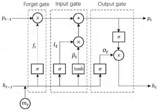
Figure 2.
Diagram of LSTM (Long Short-Term Memory) network structure.
There are three gates in an LSTM unit: the Forgetting Gate, the Input Gate, and the Output Gate. The Forgetting Gate and the Input Gate are mainly used to control the amount of information in the cell state of the previous period and the instant state generated from the current input that can be added into the current cell state . The cell state is updated based on the output of the Forgetting Gate and the Input Gate, and the hidden state is generated from the Output Gate based on the updated cell state. The calculation methods of the Forgetting Gate, the Input Gate, and the Output Gate are shown in Equations (15)–(17) respectively:
in which , and represent the results of the Forgetting Gate, the Input Gate, and the Output Gate, respectively; , and are the weight matrices of the Forgetting Gate, the Input Gate, and the Output Gate, respectively; , and are the bias terms of the Forgetting Gate, the Input Gate, and the Output Gate, respectively; is the output of the hidden layer in the previous period, and is the input at period , which is the time series data of a certain indicator of a city in this paper; is a Sigmoid function, which is defined as:
In the LSTM model, the final output is determined by the Output Gate and the cell state. The calculation methods of the instant state , the cell state , and the hidden layer output are shown in Equations (19)–(21), respectively:
in which is the instant state weight matrix; is the instant state bias term; the formula of the function is defined in Equation (22); represents the hadamard product. Assuming and are of the same order, if , the matrix is called the hadamard product of and .
After constructing the structure of LSTM, this paper has obtained a trained network by adopting an adaptive moment estimation algorithm and training the network with actual data in order to update the weights and bias terms in the network. Based on the data of the average concentration of pollutants, this paper further combines the population of each city to predict the future air pollutant data. Please refer to Appendix D for the program code of the LSTM forecast model. Moreover, the Mean Absolute Percentage Error (MAPE) values of each city are also calculated to justify the application of the LSTM forecast model (please refer to Appendix E).
3. Results
Based on the raw data introduced in Part 2.1, the PCA-TOPSIS evaluation model discussed in Part 2.2 and 2.3, and the program code presented in Appendix C, this paper has calculated the air quality evaluation scores of 16 cities in the Chengdu-Chongqing region from January 2015 to November 2019, such as shown in Figure 3, Figure 4, Figure 5, Figure 6, Figure 7, Figure 8 and Figure 9 (for detailed evaluation data, please refer to Table A1, Table A2, Table A3, Table A4, Table A5, Table A6 and Table A7 in Appendix A):
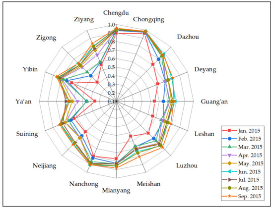
Figure 3.
The air quality evaluation scores of 16 cities in the Chengdu-Chongqing region from January 2015 to September 2015.
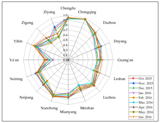
Figure 4.
The air quality evaluation scores of 16 cities in the Chengdu-Chongqing region from October 2015 to June 2016.
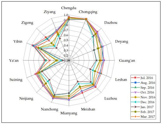
Figure 5.
The air quality evaluation scores of 16 cities in the Chengdu-Chongqing region from July 2016 to March 2017.
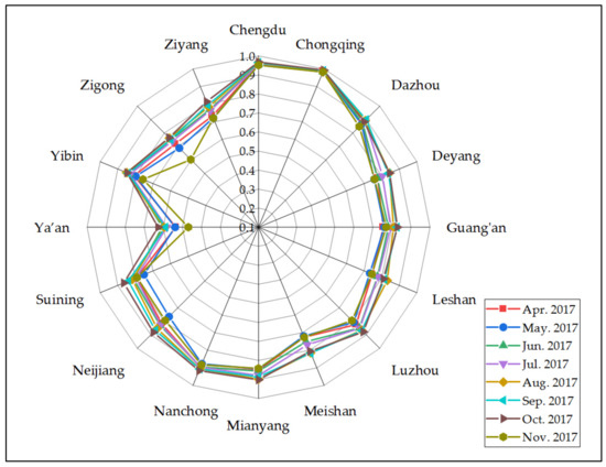
Figure 6.
The air quality evaluation scores of 16 cities in the Chengdu-Chongqing region from April 2017 to November 2017.
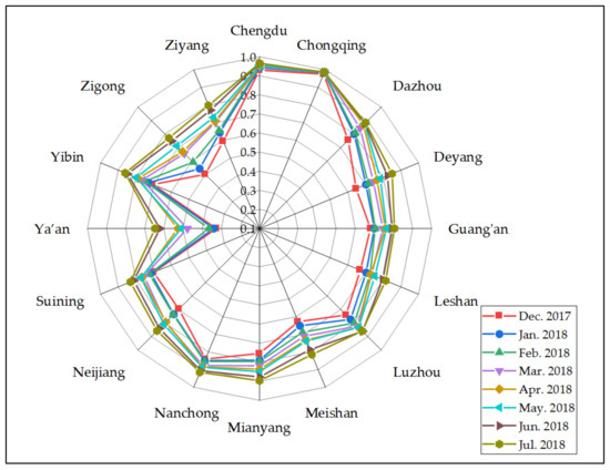
Figure 7.
The air quality evaluation scores of 16 cities in the Chengdu-Chongqing region from December 2017 to July 2018.
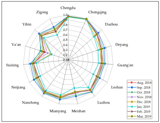
Figure 8.
The air quality evaluation scores of 16 cities in the Chengdu-Chongqing region from August 2018 to March 2019.
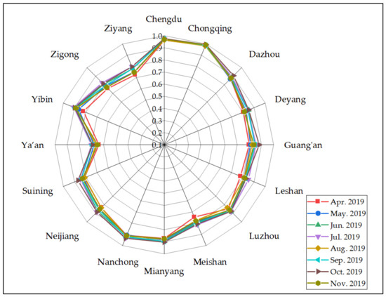
Figure 9.
The air quality evaluation scores of 16 cities in the Chengdu-Chongqing region from April 2019 to November 2019.
Further, with the help of the LSTM deep learning forecast model introduced in Part 2.4 and the program code presented in Appendix D, this paper has forecasted the air quality scores of the 16 cities in the Chengdu-Chongqing region from December 2019 to November 2020, as shown in Figure 10 and Figure 11 (for detailed evaluation data, please refer to Table A8 and Table A9 in Appendix A):
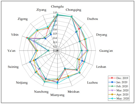
Figure 10.
The air quality forecasted scores of 16 cities in the Chengdu-Chongqing region from December 2019 to May 2020.
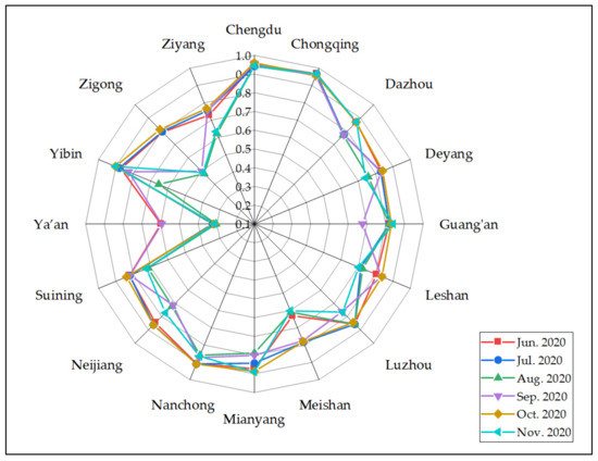
Figure 11.
The air quality forecasted scores of 16 cities in the Chengdu-Chongqing region from June 2020 to November 2020.
The above figures show the calculation results of this paper, and their specific meaning will be discussed in the next section.
4. Discussion
4.1. Analysis of Previous Effectiveness of Air Pollution Control
Based on the air quality evaluation scores of cities in the Chengdu-Chongqing region from January 2015 to November 2019 as displayed in Section 3, this paper has noticed the following characteristics in the effectiveness of air pollution control in this region:
4.1.1. Conformity
It can be seen from the evaluation results that in the research period, the year-on-year movement of historical air quality evaluation results across cities in this region was generally the same. Such conformity is mainly attributable to the following reasons: firstly, the geographical locations of cities in this area are highly similar, and these cities generally face the same external environment; secondly, the air pollution control policies of these cities have a lot in common. This region consists of two provincial administrative regions, Sichuan Province and Chongqing Municipality (directly under the central government of China). Within the research period, Sichuan Province uniformly formulated and implemented air pollution control policies which ensured coordinated and consistent air pollution control measurers across the 15 cities under its jurisdiction [74,75,76,77]. Although each city would also formulate tailored pollution control policies in accordance with their own economic and industrial characteristics, these tailored policies must be carried out under the framework of the overall provincial policies. In addition, Chongqing has been under the administrative jurisdiction of Sichuan Province from 1954 to 1997, and only became a municipality directly under the central government in 1997 [78]. Therefore, Chongqing and Sichuan Province have a lot in common in terms of their economic development stage, the external environment for air pollution control, and policy design and implementation. These factors abovementioned have resulted in the conformity in the overall trend of effectiveness of historical air pollution control policies across different cities in the Chengdu-Chongqing region.
4.1.2. Cyclicity
If analyzed by years, the effectiveness of historical air pollution control policies across the cities in this region have shown cyclical movements. The policy effectiveness usually reached its lowest level between December of the previous year and January of the current year, which gradually improved after that and climbed to the highest point from September to October of the current year, and then fell again to start the next cycle. The reason is that the air pollution control policies adopted by cities in Chengdu-Chongqing region mainly focus on industrial pollution sources and mobile pollution sources such as motor vehicles [79,80,81]. The amount of air pollutants emitted has increased as the residents’ demand for heating in winter increases [82,83], which has weakened the effects of control policies to a certain extent. In spring and summer, with less air pollution generated by heating, the air pollution control policies have shown stronger positive impact [84].
4.1.3. Improvement
It can be seen from year-on-year comparison that there is an improving trend in the air pollution levels indicating the increasing effectiveness of air pollution control measures across the cities (please refer to Table A1, Table A2, Table A3, Table A4, Table A5, Table A6 and Table A7 in Appendix A). Taking Ya’an, which has the relatively lowest evaluation scores during the survey period, as an example, its lowest air quality evaluation score has improved from 0.3494 in 2015 to 0.4504 in 2019, and its highest air quality evaluation score has increased from 0.6889 to 0.7002. As for Zigong, where the air quality evaluation score is relatively low, its lowest air quality evaluation score has also improved from 0.4160 in 2015 to 0.6429 in 2019, and the highest score has improved from 0.7286 to 0.8236. The rest of the cities have also shown improvements of varying degrees, indicating that the cities in this region have achieved significant results in air pollution control and treatment.
4.1.4. Air Pollution Control Policies in Key Cities and Their Effectiveness
- (1)
- ChengduChengdu is the capital city of Sichuan Province, as well as the economic center and air pollution control center of the province. It can be seen from the historical data that Chengdu has achieved significant air quality improvements within the research period, with its air quality score rising from 0.8960 in January 2015 to 0.9700 in November 2019, an improvement of 8.26%. Even compared with the score of January 2019 (0.9532), there has been an improvement of 1.76%. At the same time, except for 2016, the air quality of Chengdu has been improving during the research period. In order to combat air pollution, Chengdu set up an emergency command office for heavy pollution in 2014, which is responsible for coordinating and leading air pollution control campaigns in the city as well as pollution control policy implementation. In 2015, Chengdu strictly enforced the “Measures for Public Participation in Environmental Protection” [85], and continuously improved the details through implementation, which expanded the participants in environmental protection from the government and enterprises to the general public and tried to encourage the attention and involvement of the public in air pollution control. As Chengdu is located in the Sichuan Basin with a fragile environment, it suffers more from air pollution incidents compared with other regions in China. Therefore, the local government has further developed an emergency response system in order to quickly and professionally handle air pollution incidents and minimize the negative impact of sudden pollution events. Chengdu has put great emphasis on controlling the sources of air pollution. It has stipulated restricted zones for heavy-pollution fuels [86], strictly limits the emission of motor vehicles, and prohibits vehicles that do not meet standards from driving on the road; during heavy pollution periods, the local government would enforce polluting enterprises to curtail or stop production [87]. These policies and measures have effectively reduced air pollution from the source.
- (2)
- ChongqingChongqing is another key city in the Chengdu-Chongqing region. It is also one of the four municipalities directly under the central government of China, thereby enjoying the same administrative level as Sichuan Province. Due to the geographical proximity and the resulting economic and cultural integration, Chongqing follows similar ideas in air pollution control policy design as the other cities in the Chengdu-Chongqing region. However, as a municipality directly under the central government, Chongqing is more independent and implements additional measures in pollution control policy design compared with other cities in the Chengdu-Chongqing region. Under the general leadership of the central government, Chongqing has come up with the concept of “Blue Sky Protection Campaign” for air pollution control [88,89].It is worth noting that in the model setting and calculation, this paper uses the average value of six pollutants based on the population of each city. Although the total emissions of air pollutants in Chengdu and Chongqing are not low, the population of them are also considerable—the population of Chengdu in 2019 is 16.5810 million [90] and that of Chongqing is 31.2432 million [91]. The above two cities have relatively high air quality evaluation values, indicating that their air pollution control policies have achieved improved air quality in the time since 2016 to the present.
4.2. Analysis of Forecasted Effectiveness of Air Pollution Control
This paper has summarized the following characteristics regarding the forecasted effectiveness of air pollution control in this region for December 2019 to November 2020:
- (1)
- The forecasted air quality still shows an improved trend in general, but the improvement has reached the policy effectiveness ceiling under existing conditions. Using January data which shows the worst air pollution levels for comparison, the forecasted policy effectiveness in January 2020 is still improved compared with that of January 2019, but only Leshan, Mianyang and Yibin’s evaluation scores have improved, while the remaining 13 cities have declined to varying degrees. Therefore, in 2020 and beyond, how to maintain and further improve the effectiveness of air pollution control policies will be a major challenge to cities in the Chengdu-Chongqing region. It can be seen from the calculation results since 2015 that the marginal effects of air pollution control policies in the Chengdu-Chongqing region are increasingly prominent, which means the policies have reached the ceiling of producing further effects. To further improve air quality, the cities need to increase the budget, and administrative resources invested, as well as work efficiency. Therefore, this has brought further challenges to the design and implementation of air pollution control policies.
- (2)
- The gap between the forecasted results for different cities is shrinking. Sichuan Province are making and carrying out the unified planning of air pollution control policies and the regional co-management of air pollution between itself and Chongqing. The “Thirteenth Five-Year Plan for Ecological Protection and Ecological Enhancement of Sichuan Province” issued in 2017 has explicitly adopted the guiding philosophy of “Coordinated Planning and Implementation” for pollution control and emphasized putting this guiding idea into practice [92]. It can be seen from the calculation results that before 2016, there were quite large differences in the policy effectiveness of cities in the region, but the gap started to shrink after 2016 and this trend is further reflected and confirmed in the forecasted results for 2020.
5. Conclusions
Based on the historical data of 16 cities in the Chengdu-Chongqing region from January 2015 to November 2019 on six major air pollutants, this paper has first evaluated the monthly air quality of different cities by using the PCA-TOPSIS Evaluation Model. Based on that, this paper has adopted the LSTM neural network model in deep learning to forecast the monthly air quality of the cities from December 2019 to November 2020 in order to show the historical effectiveness, as well as simulate future performance of the air pollution control policies of these cities. The research results indicate that:
- (1)
- In terms of historical evaluation, air quality is improving, with distinct characteristics, like seasonal cycles in the air quality are as expected, with winters showing more severe problems related to the additional energy needs for heating.
- (2)
- Based on a year-on-year comparison, there is a trend of improving air quality indicating the effectiveness of control policies across the cities. Among those cities, Ya’an’s lowest air quality evaluation score has improved from 0.3494 in 2015 to 0.4504 in 2019; Zigong’s lowest air quality score has also risen from 0.4160 in 2015 to 0.6429 in 2019. The rest of the cities have also shown improvements of varying degrees, indicating that the cities in this region have achieved significant results in air pollution control and treatment.
- (3)
- Basedon the forecasted results from December 2019 to November 2020, this paper has noticed that although the air quality still shows an improved trend, it appears to have reached the ceiling under existing conditions. Moreover, the gap between the forecasted policy effectiveness for different cities is shrinking, which places higher requirements on the future design and implementation of air pollution control policies in this region.
Based on the Chinese government’s vigorous control of air pollution in recent years, the calculations and the abovementioned policy analysis in this paper will likely help to make practical policy measures, which will reduce emissions of air pollutants in Chengdu-Chongqing region and enhance the sustainable development there.
Author Contributions
Conceptualization, W.Y. and H.G.; methodology, H.G.; software, H.G.; validation, J.W.; formal analysis, J.W.; investigation, H.G.; resources, W.Y. and X.Z.; data curation, H.G. and X.Z.; writing—original draft preparation, J.W.; writing—review and editing, W.Y. and X.Z.; visualization, J.W.; supervision, W.Y.; project administration, J.W.; funding acquisition, W.Y. All authors have read and agreed to the published version of the manuscript.
Funding
Weixin Yang was financially supported by the National and Regional Research Projects of Ministry of Education of the People’s Republic of China in 2020 (2020-N53), the Decision-making Consultation Research Key Project of Shanghai Municipal Government (2020-A-003-B), the Decision Consulting Cultivation Project of University of Shanghai for Science and Technology (2020-JCPY-01), and the Connotation Construction Project for University Think Tank of Shanghai Municipal Education Commission (2020 Xuanchuan 6-109).
Data Availability Statement
The data presented in this study are all from the statistical data officially released by China and have been explained in the text and references.
Conflicts of Interest
The authors declare no conflict of interest.
Appendix A. Air Quality Assessment Score and Forecasted Score of Cities in Chengdu-Chongqing Region
Table A1.
Air quality assessment score of cities in Chengdu-Chongqing region (January 2015 to September 2015).
Table A1.
Air quality assessment score of cities in Chengdu-Chongqing region (January 2015 to September 2015).
| Jan. 2015 | Feb. 2015 | Mar. 2015 | Apr. 2015 | May 2015 | Jun. 2015 | Jul. 2015 | Aug. 2015 | Sep. 2015 | |
|---|---|---|---|---|---|---|---|---|---|
| Chengdu | 0.8960 | 0.9284 | 0.9335 | 0.9364 | 0.9372 | 0.9479 | 0.9372 | 0.9440 | 0.9552 |
| Chongqing | 0.9586 | 0.9742 | 0.9798 | 0.9795 | 0.9836 | 0.9880 | 0.9822 | 0.9835 | 0.9872 |
| Dazhou | 0.7072 | 0.7964 | 0.8444 | 0.8730 | 0.8608 | 0.8796 | 0.8557 | 0.8568 | 0.8725 |
| Deyang | 0.6247 | 0.7178 | 0.7214 | 0.7186 | 0.7528 | 0.8012 | 0.7562 | 0.7541 | 0.8143 |
| Guang’an | 0.5471 | 0.6488 | 0.7176 | 0.7282 | 0.7435 | 0.7879 | 0.7578 | 0.7618 | 0.7710 |
| Leshan | 0.5606 | 0.6926 | 0.6678 | 0.6777 | 0.7155 | 0.7368 | 0.7403 | 0.7524 | 0.7876 |
| Luzhou | 0.6289 | 0.7166 | 0.7549 | 0.7934 | 0.8013 | 0.8373 | 0.8100 | 0.8332 | 0.8635 |
| Meishan | 0.5432 | 0.6770 | 0.6722 | 0.6977 | 0.7007 | 0.7370 | 0.7080 | 0.7532 | 0.8019 |
| Mianyang | 0.7733 | 0.8250 | 0.8340 | 0.8307 | 0.8339 | 0.8567 | 0.8344 | 0.8550 | 0.8806 |
| Nanchong | 0.7956 | 0.8186 | 0.8631 | 0.8961 | 0.8888 | 0.9073 | 0.8847 | 0.8956 | 0.9039 |
| Neijiang | 0.6109 | 0.6730 | 0.7017 | 0.6945 | 0.7046 | 0.8068 | 0.7826 | 0.7919 | 0.8158 |
| Suining | 0.6309 | 0.6734 | 0.7054 | 0.7428 | 0.7482 | 0.8052 | 0.7772 | 0.8017 | 0.8178 |
| Ya’an | 0.3494 | 0.4485 | 0.4435 | 0.5534 | 0.6168 | 0.6691 | 0.6889 | 0.6493 | 0.6616 |
| Yibin | 0.6615 | 0.7280 | 0.7679 | 0.7970 | 0.8051 | 0.8236 | 0.8155 | 0.8377 | 0.8580 |
| Zigong | 0.4160 | 0.5239 | 0.5828 | 0.6657 | 0.6844 | 0.7278 | 0.7012 | 0.7026 | 0.7286 |
| Ziyang | 0.5594 | 0.5917 | 0.5967 | 0.6873 | 0.7472 | 0.7993 | 0.7703 | 0.7954 | 0.8327 |
Table A2.
Air quality assessment score of cities in Chengdu-Chongqing region (October 2015 to June 2016).
Table A2.
Air quality assessment score of cities in Chengdu-Chongqing region (October 2015 to June 2016).
| Oct. 2015 | Nov. 2015 | Dec. 2015 | Jan. 2016 | Feb. 2016 | Mar. 2016 | Apr. 2016 | May 2016 | Jun. 2016 | |
|---|---|---|---|---|---|---|---|---|---|
| Chengdu | 0.9360 | 0.9503 | 0.9217 | 0.9357 | 0.9417 | 0.9297 | 0.9434 | 0.9458 | 0.9510 |
| Chongqing | 0.9823 | 0.9835 | 0.9778 | 0.9775 | 0.9797 | 0.9793 | 0.9853 | 0.9831 | 0.9845 |
| Dazhou | 0.8553 | 0.8563 | 0.8258 | 0.7944 | 0.8022 | 0.8185 | 0.8549 | 0.8628 | 0.8748 |
| Deyang | 0.7542 | 0.8099 | 0.6842 | 0.6791 | 0.7209 | 0.7144 | 0.7603 | 0.7908 | 0.7596 |
| Guang’an | 0.7453 | 0.7562 | 0.7050 | 0.6689 | 0.6722 | 0.6975 | 0.7363 | 0.7512 | 0.7804 |
| Leshan | 0.6940 | 0.7362 | 0.6799 | 0.6822 | 0.6859 | 0.6469 | 0.7162 | 0.7368 | 0.7780 |
| Luzhou | 0.8094 | 0.8275 | 0.8015 | 0.7910 | 0.7718 | 0.7580 | 0.8346 | 0.8069 | 0.8305 |
| Meishan | 0.6989 | 0.7603 | 0.6603 | 0.6566 | 0.7008 | 0.6435 | 0.7304 | 0.7248 | 0.7622 |
| Mianyang | 0.8417 | 0.8575 | 0.7750 | 0.7650 | 0.7921 | 0.8123 | 0.8438 | 0.8530 | 0.8428 |
| Nanchong | 0.8742 | 0.8935 | 0.8561 | 0.8475 | 0.8510 | 0.8691 | 0.8886 | 0.8850 | 0.9024 |
| Neijiang | 0.7474 | 0.8056 | 0.7407 | 0.7359 | 0.7000 | 0.7347 | 0.8013 | 0.7755 | 0.7895 |
| Suining | 0.7562 | 0.8078 | 0.7472 | 0.7184 | 0.7037 | 0.7286 | 0.7804 | 0.7443 | 0.7924 |
| Ya’an | 0.5244 | 0.4746 | 0.4117 | 0.4045 | 0.4801 | 0.4865 | 0.5566 | 0.5717 | 0.5709 |
| Yibin | 0.7954 | 0.7980 | 0.7596 | 0.7563 | 0.7680 | 0.7648 | 0.8237 | 0.8198 | 0.8590 |
| Zigong | 0.6104 | 0.6556 | 0.5786 | 0.5783 | 0.5820 | 0.6237 | 0.7166 | 0.6633 | 0.7329 |
| Ziyang | 0.7883 | 0.8160 | 0.7496 | 0.6122 | 0.5885 | 0.5992 | 0.6691 | 0.6110 | 0.6630 |
Table A3.
Air quality assessment score of cities in Chengdu-Chongqing region (July 2016 to March 2017).
Table A3.
Air quality assessment score of cities in Chengdu-Chongqing region (July 2016 to March 2017).
| Jul. 2016 | Aug. 2016 | Sep. 2016 | Oct. 2016 | Nov. 2016 | Dec. 2016 | Jan. 2017 | Feb. 2017 | Mar. 2017 | |
|---|---|---|---|---|---|---|---|---|---|
| Chengdu | 0.9563 | 0.9467 | 0.9540 | 0.9564 | 0.9311 | 0.9104 | 0.9057 | 0.9419 | 0.9542 |
| Chongqing | 0.9848 | 0.9843 | 0.9797 | 0.9882 | 0.9827 | 0.9772 | 0.9740 | 0.9815 | 0.9841 |
| Dazhou | 0.8951 | 0.8789 | 0.8422 | 0.8824 | 0.8464 | 0.7634 | 0.7872 | 0.8334 | 0.8615 |
| Deyang | 0.7942 | 0.7983 | 0.8073 | 0.8289 | 0.7291 | 0.6358 | 0.6339 | 0.7180 | 0.7782 |
| Guang’an | 0.7912 | 0.7813 | 0.7548 | 0.7765 | 0.7222 | 0.6462 | 0.6392 | 0.7081 | 0.7336 |
| Leshan | 0.7843 | 0.7540 | 0.7697 | 0.7519 | 0.6547 | 0.6102 | 0.5562 | 0.6563 | 0.7132 |
| Luzhou | 0.8430 | 0.8115 | 0.8014 | 0.8178 | 0.7787 | 0.7421 | 0.7017 | 0.7693 | 0.7892 |
| Meishan | 0.7927 | 0.7573 | 0.7589 | 0.7627 | 0.6688 | 0.6036 | 0.5521 | 0.6631 | 0.7066 |
| Mianyang | 0.8730 | 0.8759 | 0.8635 | 0.8788 | 0.8024 | 0.7491 | 0.7468 | 0.8027 | 0.8455 |
| Nanchong | 0.9135 | 0.9042 | 0.8878 | 0.9006 | 0.8778 | 0.8449 | 0.8377 | 0.8717 | 0.8851 |
| Neijiang | 0.8138 | 0.8037 | 0.8009 | 0.8050 | 0.7447 | 0.6857 | 0.6456 | 0.7416 | 0.7815 |
| Suining | 0.8087 | 0.7757 | 0.7564 | 0.8039 | 0.7558 | 0.7183 | 0.6712 | 0.7268 | 0.7930 |
| Ya’an | 0.5731 | 0.5561 | 0.5542 | 0.4785 | 0.3328 | 0.2562 | 0.2247 | 0.3515 | 0.4793 |
| Yibin | 0.8655 | 0.8506 | 0.8393 | 0.8208 | 0.7501 | 0.7188 | 0.6837 | 0.7503 | 0.7943 |
| Zigong | 0.7406 | 0.7010 | 0.7121 | 0.6561 | 0.5318 | 0.5000 | 0.4499 | 0.5829 | 0.6642 |
| Ziyang | 0.7122 | 0.7322 | 0.7443 | 0.7463 | 0.6848 | 0.6205 | 0.5684 | 0.6535 | 0.7191 |
Table A4.
Air quality assessment score of cities in Chengdu-Chongqing region (July 2016 to March 2017).
Table A4.
Air quality assessment score of cities in Chengdu-Chongqing region (July 2016 to March 2017).
| Apr. 2017 | May 2017 | Jun. 2017 | Jul. 2017 | Aug. 2017 | Sep. 2017 | Oct. 2017 | Nov. 2017 | |
|---|---|---|---|---|---|---|---|---|
| Chengdu | 0.9557 | 0.9527 | 0.9565 | 0.9543 | 0.9647 | 0.9656 | 0.9681 | 0.9512 |
| Chongqing | 0.9858 | 0.9838 | 0.9852 | 0.9833 | 0.9836 | 0.9907 | 0.9927 | 0.9827 |
| Dazhou | 0.8706 | 0.8647 | 0.8731 | 0.8905 | 0.8929 | 0.8993 | 0.8835 | 0.8478 |
| Deyang | 0.7763 | 0.7577 | 0.7753 | 0.8044 | 0.8443 | 0.8378 | 0.8445 | 0.7593 |
| Guang’an | 0.7552 | 0.7600 | 0.7813 | 0.7929 | 0.8082 | 0.8270 | 0.8293 | 0.7701 |
| Leshan | 0.7460 | 0.7321 | 0.7761 | 0.7795 | 0.8313 | 0.8154 | 0.8098 | 0.7441 |
| Luzhou | 0.8242 | 0.8064 | 0.8487 | 0.8516 | 0.8650 | 0.8682 | 0.8774 | 0.7936 |
| Meishan | 0.7252 | 0.7195 | 0.7512 | 0.7685 | 0.8143 | 0.8160 | 0.8061 | 0.7266 |
| Mianyang | 0.8520 | 0.8451 | 0.8560 | 0.8795 | 0.8982 | 0.8864 | 0.9018 | 0.8421 |
| Nanchong | 0.8972 | 0.8770 | 0.8950 | 0.8956 | 0.9060 | 0.9063 | 0.9158 | 0.8827 |
| Neijiang | 0.8178 | 0.7647 | 0.8310 | 0.8261 | 0.8531 | 0.8663 | 0.8812 | 0.7930 |
| Suining | 0.7923 | 0.7512 | 0.8101 | 0.7971 | 0.8171 | 0.8394 | 0.8659 | 0.7901 |
| Ya’an | 0.5345 | 0.5384 | 0.6051 | 0.5825 | 0.5960 | 0.5883 | 0.6277 | 0.4688 |
| Yibin | 0.8072 | 0.7978 | 0.8322 | 0.8306 | 0.8491 | 0.8403 | 0.8470 | 0.7567 |
| Zigong | 0.7188 | 0.6882 | 0.7494 | 0.7399 | 0.7618 | 0.7515 | 0.7650 | 0.6024 |
| Ziyang | 0.7326 | 0.7205 | 0.7692 | 0.7630 | 0.7840 | 0.7948 | 0.8140 | 0.7199 |
Table A5.
Air quality assessment score of cities in Chengdu-Chongqing region (December 2018 to July 2018).
Table A5.
Air quality assessment score of cities in Chengdu-Chongqing region (December 2018 to July 2018).
| Dec. 2017 | Jan. 2018 | Feb. 2018 | Mar. 2018 | Apr. 2018 | May 2018 | Jun. 2018 | Jul. 2018 | |
|---|---|---|---|---|---|---|---|---|
| Chengdu | 0.9297 | 0.9417 | 0.9485 | 0.9474 | 0.9514 | 0.9553 | 0.9647 | 0.9660 |
| Chongqing | 0.9749 | 0.9825 | 0.9836 | 0.9872 | 0.9864 | 0.9860 | 0.9858 | 0.9856 |
| Dazhou | 0.7552 | 0.7991 | 0.8082 | 0.8431 | 0.8685 | 0.8783 | 0.8792 | 0.8839 |
| Deyang | 0.6462 | 0.7023 | 0.7153 | 0.7436 | 0.7649 | 0.7834 | 0.8237 | 0.8498 |
| Guang’an | 0.6804 | 0.7000 | 0.7046 | 0.7446 | 0.7578 | 0.7642 | 0.7922 | 0.8053 |
| Leshan | 0.6699 | 0.7032 | 0.7252 | 0.7331 | 0.7289 | 0.7520 | 0.7967 | 0.8138 |
| Luzhou | 0.7399 | 0.7729 | 0.7998 | 0.8230 | 0.8334 | 0.8321 | 0.8612 | 0.8589 |
| Meishan | 0.6282 | 0.6512 | 0.6883 | 0.7103 | 0.7325 | 0.7378 | 0.7867 | 0.8144 |
| Mianyang | 0.7544 | 0.7895 | 0.7957 | 0.8185 | 0.8371 | 0.8503 | 0.8777 | 0.8969 |
| Nanchong | 0.8398 | 0.8496 | 0.8535 | 0.8760 | 0.8835 | 0.8864 | 0.9056 | 0.9148 |
| Neijiang | 0.6968 | 0.7352 | 0.7376 | 0.7948 | 0.7937 | 0.8081 | 0.8403 | 0.8580 |
| Suining | 0.6994 | 0.7141 | 0.7245 | 0.7534 | 0.7672 | 0.7711 | 0.8120 | 0.8310 |
| Ya’an | 0.3262 | 0.3394 | 0.3651 | 0.4775 | 0.5273 | 0.5102 | 0.6209 | 0.6464 |
| Yibin | 0.7041 | 0.7282 | 0.7482 | 0.7645 | 0.7869 | 0.7981 | 0.8477 | 0.8602 |
| Zigong | 0.5014 | 0.5436 | 0.5917 | 0.6556 | 0.6687 | 0.7116 | 0.7479 | 0.7701 |
| Ziyang | 0.5950 | 0.6435 | 0.6544 | 0.7021 | 0.7094 | 0.7295 | 0.7705 | 0.7976 |
Table A6.
Air quality assessment score of cities in Chengdu-Chongqing region (August 2018 to March 2019).
Table A6.
Air quality assessment score of cities in Chengdu-Chongqing region (August 2018 to March 2019).
| Aug. 2018 | Sep. 2018 | Oct. 2018 | Nov. 2018 | Dec. 2018 | Jan. 2019 | Feb. 2019 | Mar. 2019 | |
|---|---|---|---|---|---|---|---|---|
| Chengdu | 0.9585 | 0.9731 | 0.9680 | 0.9623 | 0.9566 | 0.9532 | 0.9665 | 0.9663 |
| Chongqing | 0.9816 | 0.9933 | 0.9923 | 0.9888 | 0.9881 | 0.9804 | 0.9891 | 0.9880 |
| Dazhou | 0.8688 | 0.9028 | 0.8803 | 0.8886 | 0.8176 | 0.7901 | 0.8624 | 0.8581 |
| Deyang | 0.8054 | 0.8635 | 0.8321 | 0.7976 | 0.7670 | 0.7261 | 0.7886 | 0.7950 |
| Guang’an | 0.7729 | 0.8351 | 0.8186 | 0.7993 | 0.7630 | 0.7140 | 0.7613 | 0.7927 |
| Leshan | 0.7856 | 0.8229 | 0.7963 | 0.7838 | 0.7506 | 0.6753 | 0.7580 | 0.7762 |
| Luzhou | 0.8564 | 0.8926 | 0.8850 | 0.8411 | 0.8394 | 0.7789 | 0.8382 | 0.8354 |
| Meishan | 0.7718 | 0.8440 | 0.8188 | 0.7816 | 0.7484 | 0.6737 | 0.7563 | 0.7618 |
| Mianyang | 0.8765 | 0.9088 | 0.8839 | 0.8615 | 0.8395 | 0.8171 | 0.8627 | 0.8649 |
| Nanchong | 0.9025 | 0.9262 | 0.9122 | 0.9062 | 0.8796 | 0.8543 | 0.8882 | 0.9084 |
| Neijiang | 0.8246 | 0.8888 | 0.8562 | 0.8256 | 0.7975 | 0.7481 | 0.7867 | 0.8207 |
| Suining | 0.7914 | 0.8605 | 0.8335 | 0.8194 | 0.7913 | 0.7447 | 0.7934 | 0.8185 |
| Ya’an | 0.5895 | 0.6702 | 0.6840 | 0.5369 | 0.4623 | 0.4504 | 0.6084 | 0.6405 |
| Yibin | 0.8508 | 0.8786 | 0.8585 | 0.8202 | 0.8150 | 0.7516 | 0.8194 | 0.8186 |
| Zigong | 0.7493 | 0.8153 | 0.7981 | 0.7192 | 0.7117 | 0.6429 | 0.7240 | 0.7635 |
| Ziyang | 0.7287 | 0.8309 | 0.7939 | 0.7370 | 0.6798 | 0.5794 | 0.6746 | 0.7184 |
Table A7.
Air quality assessment score of cities in Chengdu-Chongqing region (April 2018 to November 2019).
Table A7.
Air quality assessment score of cities in Chengdu-Chongqing region (April 2018 to November 2019).
| Apr. 2019 | May 2019 | Jun. 2019 | Jul. 2019 | Aug. 2019 | Sep. 2019 | Oct. 2019 | Nov. 2019 | |
|---|---|---|---|---|---|---|---|---|
| Chengdu | 0.9631 | 0.9684 | 0.9720 | 0.9729 | 0.9646 | 0.9741 | 0.9758 | 0.9700 |
| Chongqing | 0.9877 | 0.9896 | 0.9902 | 0.9873 | 0.9828 | 0.9877 | 0.9938 | 0.9922 |
| Dazhou | 0.8719 | 0.8684 | 0.8820 | 0.8909 | 0.8737 | 0.8772 | 0.9057 | 0.8779 |
| Deyang | 0.8057 | 0.8296 | 0.8517 | 0.8453 | 0.8216 | 0.8447 | 0.8519 | 0.8128 |
| Guang’an | 0.7991 | 0.8097 | 0.8495 | 0.8555 | 0.8231 | 0.8481 | 0.8818 | 0.8387 |
| Leshan | 0.7791 | 0.8110 | 0.8300 | 0.8497 | 0.8113 | 0.8249 | 0.8281 | 0.8170 |
| Luzhou | 0.8458 | 0.8759 | 0.8757 | 0.8771 | 0.8345 | 0.8626 | 0.8766 | 0.8611 |
| Meishan | 0.7460 | 0.7857 | 0.7938 | 0.8136 | 0.7770 | 0.8033 | 0.8078 | 0.7815 |
| Mianyang | 0.8729 | 0.8848 | 0.8953 | 0.8957 | 0.8798 | 0.8975 | 0.9028 | 0.8754 |
| Nanchong | 0.9087 | 0.9069 | 0.9210 | 0.9322 | 0.9128 | 0.9234 | 0.9350 | 0.9118 |
| Neijiang | 0.8338 | 0.8590 | 0.8734 | 0.8843 | 0.8351 | 0.8589 | 0.8847 | 0.8500 |
| Suining | 0.8125 | 0.8198 | 0.8428 | 0.8461 | 0.8086 | 0.8393 | 0.8693 | 0.8293 |
| Ya’an | 0.6385 | 0.6782 | 0.6921 | 0.7002 | 0.6631 | 0.6946 | 0.6905 | 0.6495 |
| Yibin | 0.8209 | 0.8638 | 0.8904 | 0.9065 | 0.8842 | 0.8945 | 0.8993 | 0.8897 |
| Zigong | 0.7569 | 0.7838 | 0.8056 | 0.8236 | 0.7717 | 0.7880 | 0.8122 | 0.7710 |
| Ziyang | 0.7251 | 0.7502 | 0.7796 | 0.7969 | 0.7476 | 0.7806 | 0.7967 | 0.7473 |
Table A8.
Air quality forecasted score of cities in Chengdu-Chongqing region (December 2019 to May 2020).
Table A8.
Air quality forecasted score of cities in Chengdu-Chongqing region (December 2019 to May 2020).
| Dec. 2019 | Jan. 2020 | Feb. 2020 | Mar. 2020 | Apr. 2020 | May 2020 | |
|---|---|---|---|---|---|---|
| Chengdu | 0.9331 | 0.9297 | 0.9375 | 0.9499 | 0.9475 | 0.9504 |
| Chongqing | 0.9634 | 0.9631 | 0.9602 | 0.9673 | 0.9647 | 0.9652 |
| Dazhou | 0.8214 | 0.7220 | 0.7424 | 0.8510 | 0.8648 | 0.8591 |
| Deyang | 0.6722 | 0.6637 | 0.6692 | 0.7897 | 0.7957 | 0.8188 |
| Guang’an | 0.8128 | 0.6698 | 0.6602 | 0.7805 | 0.8059 | 0.8048 |
| Leshan | 0.7753 | 0.7298 | 0.6126 | 0.6331 | 0.6507 | 0.7842 |
| Luzhou | 0.7512 | 0.7378 | 0.7303 | 0.8414 | 0.8317 | 0.8268 |
| Meishan | 0.5815 | 0.5552 | 0.5641 | 0.7688 | 0.7493 | 0.7773 |
| Mianyang | 0.8512 | 0.8416 | 0.7599 | 0.7743 | 0.7819 | 0.8673 |
| Nanchong | 0.8310 | 0.8160 | 0.8305 | 0.8949 | 0.8875 | 0.8927 |
| Neijiang | 0.8287 | 0.6989 | 0.6929 | 0.7186 | 0.7962 | 0.8213 |
| Suining | 0.7866 | 0.6607 | 0.7013 | 0.8063 | 0.7044 | 0.7988 |
| Ya’an | 0.6074 | 0.3202 | 0.3106 | 0.5900 | 0.5792 | 0.6006 |
| Yibin | 0.8699 | 0.8218 | 0.6914 | 0.7016 | 0.8374 | 0.8542 |
| Zigong | 0.5055 | 0.5020 | 0.5368 | 0.7781 | 0.7661 | 0.7848 |
| Ziyang | 0.6702 | 0.5105 | 0.5466 | 0.6593 | 0.6777 | 0.7071 |
Table A9.
Air quality forecasted score of cities in Chengdu-Chongqing region (June 2020 to November 2020).
Table A9.
Air quality forecasted score of cities in Chengdu-Chongqing region (June 2020 to November 2020).
| Jun. 2020 | Jul. 2020 | Aug. 2020 | Sep. 2020 | Oct. 2020 | Nov. 2020 | |
|---|---|---|---|---|---|---|
| Chengdu | 0.9527 | 0.9416 | 0.9433 | 0.9572 | 0.9600 | 0.9442 |
| Chongqing | 0.9678 | 0.9659 | 0.9609 | 0.9557 | 0.9592 | 0.9664 |
| Dazhou | 0.8684 | 0.7753 | 0.7704 | 0.7737 | 0.8680 | 0.8702 |
| Deyang | 0.8325 | 0.8294 | 0.7569 | 0.8320 | 0.8404 | 0.7412 |
| Guang’an | 0.8177 | 0.8197 | 0.8195 | 0.6765 | 0.8309 | 0.8400 |
| Leshan | 0.8050 | 0.7133 | 0.7249 | 0.8328 | 0.8361 | 0.7020 |
| Luzhou | 0.8566 | 0.8573 | 0.8565 | 0.7616 | 0.8439 | 0.7660 |
| Meishan | 0.6310 | 0.7835 | 0.6098 | 0.7746 | 0.7798 | 0.6019 |
| Mianyang | 0.8726 | 0.8432 | 0.7888 | 0.8016 | 0.8869 | 0.8900 |
| Nanchong | 0.9069 | 0.9088 | 0.8588 | 0.8719 | 0.9096 | 0.8646 |
| Neijiang | 0.8467 | 0.8610 | 0.7209 | 0.7135 | 0.8616 | 0.7716 |
| Suining | 0.8215 | 0.8195 | 0.7144 | 0.8176 | 0.8381 | 0.7230 |
| Ya’an | 0.5988 | 0.3236 | 0.3049 | 0.5943 | 0.3169 | 0.3134 |
| Yibin | 0.8707 | 0.8800 | 0.6527 | 0.8265 | 0.9019 | 0.9008 |
| Zigong | 0.7929 | 0.7963 | 0.4792 | 0.4980 | 0.8126 | 0.4881 |
| Ziyang | 0.7289 | 0.7547 | 0.6220 | 0.7549 | 0.7665 | 0.6335 |
Appendix B. The Calculation of PCA (Principal Component Analysis) and Weights
After calculation, the eigenvalue and variance contribution percentage of each principal component can be obtained, as shown in the following Table A10:
Table A10.
The eigenvalue and variance contribution percentage of each principal component.
Table A10.
The eigenvalue and variance contribution percentage of each principal component.
| Principal Component | Eigenvalue | Variance Contribution Percentage (%) | Cumulative Variance Contribution Percentage (%) |
|---|---|---|---|
| 4.3887 | 73.1442 | 73.1442 | |
| 0.9255 | 15.4256 | 88.5698 | |
| 0.3281 | 5.4679 | 94.0377 | |
| 0.1906 | 3.1771 | 97.2148 | |
| 0.1431 | 2.3843 | 99.5991 | |
| 0.0241 | 0.4009 | 100.0000 |
It can be seen that the sum of the cumulative contribution percentage of the first two principal components and to the whole has reached more than 85%, so this article selects the first two principal components for the subsequent assignment of indicators. The principal component load matrix is shown in the following Table A11:
Table A11.
The principal component load matrix of six pollutants.
Table A11.
The principal component load matrix of six pollutants.
| PM2.5 | 0.9527 | 0.9416 | 0.9433 | 0.9572 | 0.9600 | 0.9442 |
| PM10 | 0.9678 | 0.9659 | 0.9609 | 0.9557 | 0.9592 | 0.9664 |
| SO2 | 0.5988 | 0.3236 | 0.3049 | 0.5943 | 0.3169 | 0.3134 |
| NO2 | 0.8707 | 0.8800 | 0.6527 | 0.8265 | 0.9019 | 0.9008 |
| O3 | 0.7929 | 0.7963 | 0.4792 | 0.4980 | 0.8126 | 0.4881 |
| CO | 0.7289 | 0.7547 | 0.6220 | 0.7549 | 0.7665 | 0.6335 |
Finally, the weights of the six pollutants can be obtained, as shown in the following Table A12:
Table A12.
The weights of the six pollutants.
Table A12.
The weights of the six pollutants.
| PM2.5 | PM10 | SO2 | NO2 | O3 | CO | |
|---|---|---|---|---|---|---|
| Weight | 0.1797 | 0.1785 | 0.1634 | 0.1628 | 0.1565 | 0.1591 |
Appendix C. The MATLAB Algorithm for the PCA-TOPSIS Model
| Algorithm A1 PCA-TOPSIS. | |
| 1: | function [T]=PCA_TOPSIS(b) |
| 2: | x=zscore(b); |
| 3: | [coeff,score,latent,tsquare]=pca(x); |
| 4: | y=(100*latent/sum(latent))’; |
| 5: | y_s=y(1); |
| 6: | n=1; |
| 7: | if y_s<85 |
| 8: | n=n+1; |
| 9: | y_s=y(n)+y_s; |
| 10: | end |
| 11: | coeff_abs=abs(coeff(:,1:n)); |
| 12: | for i=1:n |
| 13: | if i==1 |
| 14: | weight=y(1)*coeff_abs(:,1); |
| 15: | else |
| 16: | weight=weight+y(i)*coeff_abs(:,i); |
| 17: | end |
| 18: | end |
| 19: | weight=weight/sum(weight); |
| 20: | [m,n]=size(b); |
| 21: | for i=1:n |
| 22: | s=0; |
| 23: | for j=1:m |
| 24: | s=s+b(j,i)^2; |
| 25: | if j==m |
| 26: | s=sqrt(s); |
| 27: | end |
| 28: | end |
| 29: | b(:,i)= b(:,i)/s; |
| 30: | b(:,i)=b(:,i)*weight(i); |
| 31: | end |
| 32: | v1=max(b); |
| 33: | v2=min(b); |
| 34: | T=zeros(m,1); |
| 35: | for i=1:m |
| 36: | C1=b(i,:)-v1; |
| 37: | S1=norm(C1); |
| 38: | C2=b(i,:)-v2; |
| 39: | S2=norm(C2); |
| 40: | T(i)=S1/(S1+S2); |
| 41: | end |
Appendix D. The MATLAB Algorithm for the LSTM Model
| Algorithm A2 LSTM | |
| 1: | function [dataPred]=LSTM(data,population,P_t,lL,fCL,ME,GT,ILR,LRDP,LRDF) |
| 2: | mu = mean(data); |
| 3: | sig = std(data); |
| 4: | dataStandardized = (data-mu)/sig; |
| 5: | populationStandardized = (population-mean(population))/std(population); |
| 6: | XTrain = zeros(2,length(dataStandardized)-1); |
| 7: | XTrain(1,:) = dataStandardized(1:end-1); |
| 8: | XTrain(2,:) = populationStandardized(2: length(dataStandardized)) |
| 9: | YTrain = dataStandardized(2:end); |
| 10: | layers = [... |
| 11: | sequenceInputLayer(2) |
| 12: | lstmLayer(lL) |
| 13: | fullyConnectedLayer(fCL) |
| 14: | regressionLayer]; |
| 15: | options = trainingOptions(‘adam’, ... |
| 16: | ‘MaxEpochs’,ME, ... |
| 17: | ‘GradientThreshold’,GT, ... |
| 18: | ‘InitialLearnRate’,ILR, ... |
| 19: | ‘LearnRateSchedule’,’piecewise’, ... |
| 20: | ‘LearnRateDropPeriod’,LRDP, ... |
| 21: | ‘LearnRateDropFactor’,LRDF, ... |
| 22: | ‘Verbose’,0, ... |
| 23: | ‘Plots’,’training-progress’); |
| 24: | net = trainNetwork(XTrain,YTrain,layers,options); |
| 25: | net = predictAndUpdateState(net,XTrain); |
| 26: | [net,dataPred]=predictAndUpdateState(net,[YTrain(end);populationStandardized(length(dataStandardized)+1)]); |
| 27: | numTimeStepsPred = P_t; |
| 28: | for i = 2:numTimeStepsPred |
| 29: | [net,dataPred(:,i)]=predictAndUpdateState(net,[dataPred(:,i-1); |
| 30: | populationStandardized(length(dataStandardized)+i)]); |
| 31: | end |
| 32: | dataPred = sig*dataPred + mu; |
Appendix E. The Mean Absolute Percentage Error (MAPE) of LSTM Forecast Model
The research sample in this paper contains a total of 59 months of data. Here, the data of the first 48 months is used as the training set, and the data of the next 11 months is used as the verification set. The Mean Absolute Percentage Error (MAPE) is used to evaluate the training results of LSTM forecast model (please refer to the following Table A13):
Table A13.
The Mean Absolute Percentage Error (MAPE) of cities in Chengdu-Chongqing region.
Table A13.
The Mean Absolute Percentage Error (MAPE) of cities in Chengdu-Chongqing region.
| City | Mean Absolute Percentage Error (MAPE) |
|---|---|
| Chengdu | 0.1099 |
| Chongqing | 0.1443 |
| Dazhou | 0.1570 |
| Deyang | 0.1634 |
| Guang’an | 0.1670 |
| Leshan | 0.1670 |
| Luzhou | 0.1639 |
| Meishan | 0.1110 |
| Mianyang | 0.1068 |
| Nanchong | 0.1675 |
| Neijiang | 0.1383 |
| Suining | 0.1195 |
| Ya’an | 0.1340 |
| Yibin | 0.1679 |
| Zigong | 0.1089 |
| Ziyang | 0.1560 |
According to the above calculation results, the MAPE value of each city is low, indicating that the LSTM forecast model can predict the future trend of air quality in cities in Chengdu-Chongqing region well [93,94].
References
- Yang, W.; Yang, Y. Research on Air Pollution Control in China: From the Perspective of Quadrilateral Evolutionary Games. Sustainability 2020, 12, 1756. [Google Scholar] [CrossRef]
- Li, L.; Yang, W. Total Factor Efficiency Study on China’s Industrial Coal Input and Wastewater Control with Dual Target Variables. Sustainability 2018, 10, 2121. [Google Scholar] [CrossRef]
- Yang, W.; Li, L. Energy Efficiency, Ownership Structure, and Sustainable Development: Evidence from China. Sustainability 2017, 9, 912. [Google Scholar] [CrossRef]
- Peng, Y.; Cui, J.; Cao, Y.; Du, Y.; Chan, A.; Yang, F.; Yang, H. Impact of Manufacturing Transfer on SO2 Emissions in Jiangsu Province, China. Atmosphere 2016, 7, 69. [Google Scholar] [CrossRef]
- Gao, H.; Yang, W.; Yang, Y.; Yuan, G. Analysis of the Air Quality and the Effect of Governance Policies in China’s Pearl River Delta, 2015–2018. Atmosphere 2019, 10, 412. [Google Scholar] [CrossRef]
- Huang, Z.; Yu, Q.; Liu, Y.; Ma, W.; Chen, L. Optimal Design of Air Quality Monitoring Network for Pollution Detection and Source Identification in Industrial Parks. Atmosphere 2019, 10, 318. [Google Scholar] [CrossRef]
- Yang, W.; Yuan, G.; Han, J. Is China’s air pollution control policy effective? Evidence from Yangtze River Delta cities. J. Clean. Prod. 2019, 220, 110–133. [Google Scholar] [CrossRef]
- Yuan, G.; Yang, W. Evaluating China’s Air Pollution Control Policy with Extended AQI Indicator System: Example of the Beijing-Tianjin-Hebei Region. Sustainability 2019, 11, 939. [Google Scholar] [CrossRef]
- Yang, Y.; Yang, W. Does Whistleblowing Work for Air Pollution Control in China? A Study Based on Three-party Evolutionary Game Model under Incomplete Information. Sustainability 2019, 11, 324. [Google Scholar] [CrossRef]
- Zhao, A.; Li, Z.; Zhang, Y.; Zhang, Y.; Li, D. Merging MODIS and Ground-Based Fine Mode Fraction of Aerosols Based on the Geostatistical Data Fusion Method. Atmosphere 2017, 8, 117. [Google Scholar] [CrossRef]
- Zhang, D.; Pan, S.L.; Yu, J.; Liu, W. Orchestrating big data analytics capability for sustainability: A study of air pollution management in China. Inf. Manag. 2019, 103231. [Google Scholar] [CrossRef]
- Yuan, G.; Yang, W. Study on optimization of economic dispatching of electric power system based on Hybrid Intelligent Algorithms (PSO and AFSA). Energy 2019, 183, 926–935. [Google Scholar] [CrossRef]
- Li, Y.; Yang, W.; Shen, X.; Yuan, G.; Wang, J. Water Environment Management and Performance Evaluation in Central China: A Research Based on Comprehensive Evaluation System. Water 2019, 11, 2472. [Google Scholar] [CrossRef]
- Feng, Y.; Ning, M.; Lei, Y.; Sun, Y.; Liu, W.; Wang, J. Defending blue sky in China: Effectiveness of the “Air Pollution Prevention and Control Action Plan” on air quality improvements from 2013 to 2017. J. Environ. Manage. 2019, 252, 109603. [Google Scholar] [CrossRef] [PubMed]
- Central Committee of the Communist Party of China. Constitution of the Communist Party of China; China Legal System Publishing House: Beijing, China, 2018. [Google Scholar]
- The National People’s Congress of the People’s Republic of China. Constitution of the People’s Republic of China. Available online: http://www.gov.cn/guoqing/2018-03/22/content_5276318.htm (accessed on 25 April 2020).
- Yan, L.; Duarte, F.; Wang, D.; Zheng, S.; Ratti, C. Exploring the effect of air pollution on social activity in China using geotagged social media check-in data. Cities 2019, 91, 116–125. [Google Scholar] [CrossRef]
- Dong, R.; Fisman, R.; Wang, Y.; Xu, N. Air pollution, affect, and forecasting bias: Evidence from Chinese financial analysts. J. Financ. Econ. 2019. [Google Scholar] [CrossRef]
- Dewan, N.; Wang, Y.; Zhang, Y.; Zhang, Y.; He, L.; Huang, X.; Majestic, B.J. Effect of Pollution Controls on Atmospheric PM2.5 Composition during Universiade in Shenzhen, China. Atmosphere 2016, 7, 57. [Google Scholar] [CrossRef]
- Yang, W.; Li, L. Efficiency Evaluation and Policy Analysis of Industrial Wastewater Control in China. Energies 2017, 10, 1201. [Google Scholar] [CrossRef]
- Li, N.; Zhang, X.; Shi, M.; Hewings, G.J.D. Does China’s air pollution abatement policy matter? An assessment of the Beijing-Tianjin-Hebei region based on a multi-regional CGE model. Energy Policy 2019, 127, 213–227. [Google Scholar] [CrossRef]
- Xiao, C.; Chang, M.; Guo, P.; Gu, M.; Li, Y. Analysis of air quality characteristics of Beijing–Tianjin–Hebei and its surrounding air pollution transport channel cities in China. J. Environ. Sci. 2020, 87, 213–227. [Google Scholar] [CrossRef]
- Yun, G.; He, Y.; Jiang, Y.; Dou, P.; Dai, S. PM2.5 Spatiotemporal Evolution and Drivers in the Yangtze River Delta between 2005 and 2015. Atmosphere 2019, 10, 55. [Google Scholar] [CrossRef]
- Bao, M.; Cao, F.; Chang, Y.; Zhang, Y.-L.; Gao, Y.; Liu, X.; Zhang, Y.; Zhang, W.; Tang, T.; Xu, Z.; et al. Characteristics and origins of air pollutants and carbonaceous aerosols during wintertime haze episodes at a rural site in the Yangtze River Delta, China. Atmos. Pollut. Res. 2017, 8, 900–911. [Google Scholar] [CrossRef]
- Wu, Z.; Zhang, Y.; Zhang, L.; Huang, M.; Zhong, L.; Chen, D.; Wang, X. Trends of outdoor air pollution and the impact on premature mortality in the Pearl River Delta region of southern China during 2006–2015. Sci. Total Environ. 2019, 690, 248–260. [Google Scholar] [CrossRef] [PubMed]
- Xie, J.; Liao, Z.; Fang, X.; Xu, X.; Wang, Y.; Zhang, Y.; Liu, J.; Fan, S.; Wang, B. The characteristics of hourly wind field and its impacts on air quality in the Pearl River Delta region during 2013–2017. Atmos. Res. 2019, 227, 112–124. [Google Scholar] [CrossRef]
- Zhou, Y.; Luo, B.; Li, J.; Hao, Y.; Yang, W.; Shi, F.; Chen, Y.; Simayi, M.; Xie, S. Characteristics of six criteria air pollutants before, during, and after a severe air pollution episode caused by biomass burning in the southern Sichuan Basin, China. Atmos. Environ. 2019, 215, 116840. [Google Scholar] [CrossRef]
- Mavrakou, T.; Philippopoulos, K.; Deligiorgi, D. The impact of sea breeze under different synoptic patterns on air pollution within Athens basin. Sci. Total Environ. 2012, 433, 31–43. [Google Scholar] [CrossRef]
- Yang, W.; Li, L. Efficiency evaluation of industrial waste gas control in China: A study based on data envelopment analysis (DEA) model. J. Clean. Prod. 2018, 179, 1–11. [Google Scholar] [CrossRef]
- Zhang, C.Y.; Zhang, A. Climate and air pollution alter incidence of tuberculosis in Beijing, China. Ann. Epidemiol. 2019, 37, 71–76. [Google Scholar] [CrossRef]
- Wang, N.; Mengersen, K.; Tong, S.; Kimlin, M.; Zhou, M.; Wang, L.; Yin, P.; Xu, Z.; Cheng, J.; Zhang, Y.; et al. Short-term association between ambient air pollution and lung cancer mortality. Environ. Res. 2019, 179, 108748. [Google Scholar] [CrossRef]
- Salthammer, T.; Uhde, E.; Schripp, T.; Schieweck, A.; Morawska, L.; Mazaheri, M.; Clifford, S.; He, C.; Buonanno, G.; Querol, X.; et al. Children’s well-being at schools: Impact of climatic conditions and air pollution. Environ. Int. 2016, 94, 196–210. [Google Scholar] [CrossRef]
- Hirel, C.; Berton, L.; Preda, C.; Richard, O.; Lambert, Y.; Pico, F. Air pollution and humidity as triggering factors for stroke. Results of a 12-year analysis in the West Paris area. Rev. Neurol. 2019, 175, 614–618. [Google Scholar] [CrossRef] [PubMed]
- Shen, X.; Yang, W.; Sun, S. Analysis of the Impact of China’s Hierarchical Medical System and Online Appointment Diagnosis System on the Sustainable Development of Public Health: A Case Study of Shanghai. Sustainability 2019, 11, 6564. [Google Scholar] [CrossRef]
- Ning, G. Meteorological Causes of Air Pollution in the Northwest Urban Agglomeration of Sichuan Basin in Winter and Their Numerical Simulation; Lanzhou University: Lanzhou, China, 2018. [Google Scholar]
- National Bureau of Statistics of China. China Statistical Yearbook, 2000–2018; China Statistic Press: Beijing, China, 2019. [Google Scholar]
- Qin, B. City profile: Chengdu. Cities 2015, 43, 18–27. [Google Scholar] [CrossRef]
- Bao, H.X.H.; Li, L.; Lizieri, C. City profile: Chongqing (1997–2017). Cities 2019, 94, 161–171. [Google Scholar] [CrossRef]
- Statistics Bureau of Sichuan Province. Sichuan Statistical Yearbook, 2005–2018; China Statistic Press: Beijing, China, 2019. [Google Scholar]
- Wu, Z.; Zhao, C.; Chen, M. Research on Scientific & Technological Achievements Transformation of Sichuan Provincial State-Owned Enterprises of China. Am. J. Ind. Bus. Manag. 2016, 6, 815. [Google Scholar]
- Wang, Q.; Zhan, L. Assessing the sustainability of the shale gas industry by combining DPSIRM model and RAGA-PP techniques: An empirical analysis of Sichuan and Chongqing, China. Energy 2019, 176, 353–364. [Google Scholar] [CrossRef]
- Yang, W.X.; Li, L.G. Analysis of total factor efficiency of water resource and energy in China: A study based on DEA-SBM model. Sustainability 2017, 9, 1316. [Google Scholar] [CrossRef]
- Chalabi, Z.; Milojevic, A.; Doherty, R.M.; Stevenson, D.S.; MacKenzie, I.A.; Milner, J.; Vieno, M.; Williams, M.; Wilkinson, P. Applying air pollution modelling within a multi-criteria decision analysis framework to evaluate UK air quality policies. Atmos. Environ. 2017, 167, 466–475. [Google Scholar] [CrossRef]
- Wang, Q.; Dai, H.; Wang, H. A Smart MCDM Framework to Evaluate the Impact of Air Pollution on City Sustainability: A Case Study from China. Sustainability 2017, 9, 911. [Google Scholar] [CrossRef]
- Caravaggio, N.; Caravella, S.; Ishizaka, A.; Resce, G. Beyond CO2: A multi-criteria analysis of air pollution in Europe. J. Clean. Prod. 2019, 219, 576–586. [Google Scholar] [CrossRef]
- Chen, K.; Yien, J.; Chiang, C.; Tsai, P.; Tsai, F. Identifying Key Sources of City Air Quality: A Hybrid MCDM Model and Improvement Strategies. Appl. Sci. 2019, 9, 1414. [Google Scholar] [CrossRef]
- Chauvy, R.; Lepore, R.; Fortemps, P.; Weireld, G.D.E. Comparison of multi-criteria decision-analysis methods for selecting carbon dioxide utilization products. Sustain. Prod. Consum. 2020, 24, 194–210. [Google Scholar] [CrossRef]
- Alimissis, A.; Philippopoulos, K.; Tzanis, C.G.; Deligiorgi, D. Spatial estimation of urban air pollution with the use of artificial neural network models. Atmos. Environ. 2018, 191, 205–213. [Google Scholar] [CrossRef]
- Zhao, J.; Deng, F.; Cai, Y.; Chen, J. Long short-term memory—Fully connected (LSTM-FC) neural network for PM2.5 concentration prediction. Chemosphere 2019, 220, 486–492. [Google Scholar] [CrossRef] [PubMed]
- Zhou, Y.; Chang, F.; Chang, L.; Kao, I.; Wang, Y. Explore a deep learning multi-output neural network for regional multi-step-ahead air quality forecasts. J. Clean. Prod. 2019, 209, 134–145. [Google Scholar] [CrossRef]
- Maleki, H.; Sorooshian, A.; Goudarzi, G.; Baboli, Z.; Tahmasebi Birgani, Y.; Rahmati, M. Air pollution prediction by using an artificial neural network model. Clean Technol. Environ. Policy 2019, 21, 1341–1352. [Google Scholar] [CrossRef]
- Fong, I.H.; Li, T.; Fong, S.; Wong, R.K.; Tallón Ballesteros, A.J. Predicting concentration levels of air pollutants by transfer learning and recurrent neural network. Knowl. Based Syst. 2020, 192, 105622. [Google Scholar] [CrossRef]
- Ministry of Environmental Protection of the People’s Republic of China. Ambient Air Quality Standards: GB3095-2012; China Environmental Science Press: Beijing, China, 2012. [Google Scholar]
- Ministry of Environmental Protection of the People’s Republic of China. Technical Regulation on Ambient Air Quality Index (on Trial): HJ 633-2012; China Environmental Science Press: Beijing, China, 2012. [Google Scholar]
- China National Environmental Monitoring Center. Real-time Data on Urban Air Quality in China. Available online: http://www.cnemc.cn/sssj/ (accessed on 25 April 2020).
- Data Center of China’s Ministry of Environmental Protection. National Urban Air Quality Daily, 2015–2019. Available online: http://datacenter.mee.gov.cn/websjzx/dataproduct/resourceproduct/queryDataToReport.vm?id=3&url=/websjzx/report!list.vm?xmlname=1512478367400&ftype=zyml (accessed on 25 April 2020).
- Ecological Environment Department of Sichuan Province. Daily Air Quality Report. Available online: http://sthjt.sc.gov.cn/ (accessed on 25 April 2020).
- Ecological Environment Monitoring Center of Chongqing. Real-time Release of Air Quality in Chongqing. Available online: http://113.204.96.36:3362/template/home.html (accessed on 25 April 2020).
- Tao, A.X.; Chang, B.R.; Li, C.C.; Wang, D.R.; Liu, E.R. Density-sensitive Robust Fuzzy Kernel Principal Component Analysis technique. Neurocomputing 2019, 329, 210–226. [Google Scholar] [CrossRef]
- Berradi, Z.; Lazaar, M. Integration of Principal Component Analysis and Recurrent Neural Network to Forecast the Stock Price of Casablanca Stock Exchange. Procedia Comput. Sci. 2019, 148, 55–61. [Google Scholar] [CrossRef]
- Yang, Y.; Yang, W.; Chen, H.; Li, Y. China’s energy whistleblowing and energy supervision policy: An evolutionary game perspective. Energy 2020, 213, 118774. [Google Scholar] [CrossRef]
- Gajjar, S.; Kulahci, M.; Palazoglu, A. Real-time fault detection and diagnosis using sparse principal component analysis. J. Process Control 2018, 67, 112–128. [Google Scholar] [CrossRef]
- Li, N.; Guo, S.; Wang, Y. Weighted preliminary-summation-based principal component analysis for non-Gaussian processes. Control Eng. Pract. 2019, 87, 122–132. [Google Scholar] [CrossRef]
- Hajek, P.; Froelich, W. Integrating TOPSIS with interval-valued intuitionistic fuzzy cognitive maps for effective group decision making. Inf. Sci. 2019, 485, 394–412. [Google Scholar] [CrossRef]
- Zhang, K.; Zhan, J.; Yao, Y. TOPSIS method based on a fuzzy covering approximation space: An application to biological nano-materials selection. Inf. Sci. 2019, 502, 297–329. [Google Scholar] [CrossRef]
- Sun, G.; Guan, X.; Yi, X.; Zhou, Z. An innovative TOPSIS approach based on hesitant fuzzy correlation coefficient and its applications. Appl. Soft Comput. 2018, 68, 249–267. [Google Scholar] [CrossRef]
- Reddy, B.K.; Delen, D. Predicting hospital readmission for lupus patients: An RNN-LSTM-based deep-learning methodology. Comput. Biol. Med. 2018, 101, 199–209. [Google Scholar] [CrossRef]
- Liu, H.; Liu, J.; Yang, W.; Chen, J.; Zhu, M. Analysis and Prediction of Land Use in Beijing-Tianjin-Hebei Region: A Study Based on the Improved Convolutional Neural Network Model. Sustainability 2020, 12, 3002. [Google Scholar] [CrossRef]
- Peng, Y.; Kondo, N.; Fujiura, T.; Suzuki, T.; Wulandari; Yoshioka, H.; Itoyama, E. Classification of multiple cattle behavior patterns using a recurrent neural network with long short-term memory and inertial measurement units. Comput. Electron. Agric. 2019, 157, 247–253. [Google Scholar] [CrossRef]
- Liu, Y.; Zhang, X.; Huang, F.; Tang, X.; Li, Z. Visual question answering via Attention-based syntactic structure tree-LSTM. Appl. Soft Comput. 2019, 82, 105584. [Google Scholar] [CrossRef]
- Ertam, F. An effective gender recognition approach using voice data via deeper LSTM networks. Appl. Acoust. 2019, 156, 351–358. [Google Scholar] [CrossRef]
- Xie, X.; Liu, G.; Cai, Q.; Wei, P.; Qu, H. Multi-source sequential knowledge regression by using transfer RNN units. Neural Netw. 2019, 119, 151–161. [Google Scholar] [CrossRef] [PubMed]
- Li, P.; Abdel-Aty, M.; Yuan, J. Real-time crash risk prediction on arterials based on LSTM-CNN. Accid. Anal. Prev. 2020, 135, 105371. [Google Scholar] [CrossRef] [PubMed]
- Sichuan Provincial Government. Notice on Printing and Distributing the Implementation Rules of “Sichuan Province Air Pollution Control Plan 2015”. Available online: http://www.sc.gov.cn/10462/10883/11066/2015/4/22/10333390.shtml (accessed on 25 April 2020).
- Sichuan Provincial Government. Notice on Printing and Distributing the Implementation Rules of “Sichuan Province Air Pollution Control Plan 2016”. Available online: http://www.sc.gov.cn/zcwj/xxgk/NewT.aspx?i=20160401095908-612769-00-000 (accessed on 25 April 2020).
- Sichuan Provincial Government. Notice on Printing and Distributing the Implementation Rules of “Sichuan Province Air Pollution Control Plan 2017”. Available online: http://www.sc.gov.cn/zcwj/xxgk/NewT.aspx?i=20170527091543-450025-00-000 (accessed on 25 April 2020).
- Sichuan Provincial Government. Measures in Sichuan Province for Implementing the “Air Pollution Control Law of People’s Republic of China”. Available online: http://www.sc.gov.cn/10462/10771/10795/12400/2018/3/6/10446249.shtml (accessed on 25 April 2020).
- The Fifth Session of the Eighth National People’s Congress of the People’s Republic of China. Decision of the Fifth Session of the Eighth National People’s Congress on Approving the Establishment of Chongqing Municipality. Available online: http://www.npc.gov.cn/wxzl/wxzl/2001-02/06/content_4679.htm (accessed on 25 April 2020).
- Standing Committee of Sichuan Provincial People’s Congress. Implementation Measures of Sichuan Province “The Air Pollution Prevention and Control Law of the People’s Republic of China”. Available online: http://www.npc.gov.cn/zgrdw/npc/zfjc/zfjcelys/2014-10/21/content_1881785.htm (accessed on 15 July 2020).
- The People’s Government of Sichuan Province. Implementation Measures of Sichuan Province “The Air Pollution Prevention and Control Law of the People’s Republic of China” (Revision). Available online: http://www.sc.gov.cn/10462/10771/10795/12400/2018/6/27/10454411.shtml (accessed on 15 July 2020).
- Standing Committee of Chongqing Municipal People’s Congress. Air Pollution Prevention and Control Regulations of Chongqing. Available online: http://www.ccpc.cq.cn/home/index/more/id/212734.html (accessed on 15 July 2020).
- The People’s Government of Sichuan Province. Implementation Opinions on Comprehensively Strengthening Ecological Environment Protection and Resolutely Fighting the Tough Battle of Pollution Prevention and Control. Available online: http://www.sc.gov.cn/10462/10464/10797/2018/11/26/10463649.shtml (accessed on 15 July 2020).
- Ministry of Ecology and Environment of the People’s Republic of China. Notice on Issuing the “Key Points of National Air Pollution Prevention and Control Work in 2019”. Available online: http://www.mee.gov.cn/xxgk2018/xxgk/xxgk05/201903/t20190306_694550.html (accessed on 15 July 2020).
- Chen, Y.; Xie, S.; Luo, B.; Zhai, C. Characteristics and origins of carbonaceous aerosol in the Sichuan Basin, China. Atmos. Environ. 2014, 94, 215–223. [Google Scholar] [CrossRef]
- Chengdu Ecological Environment Bureau. Measures for Public Participation in Environmental Protection. Available online: http://gk.chengdu.gov.cn/govInfoPub/detail.action?id=75826&tn=6 (accessed on 25 April 2020).
- Chengdu Ecological Environment Bureau. Notice on Delimitation of Restricted Zones for Heavy-pollution Fuels. Available online: http://gk.chengdu.gov.cn/govInfoPub/detail.action?id=71854&tn=6 (accessed on 25 April 2020).
- The Leading Group on Air Pollution Control of Chengdu. 2019 Air Pollution Prevention Work Plan of Chengdu. Available online: http://gk.chengdu.gov.cn/govInfoPub/detail.action?id=2491726&tn=2 (accessed on 25 April 2020).
- Chongqing Municipal People’s Government. Jiulongpo District of Chongqing Fights for the “Blue Sky Protection Campaign”. Available online: http://www.cq.gov.cn/zwxx/zwdt/202001/t20200114_4648106.html (accessed on 25 April 2020).
- Chongqing Municipal People’s Government. Chongqing Releases Three-Year Action Plan to Win the “Blue Sky Protection Campaign”. Available online: http://www.cq.gov.cn/zqfz/sthj/202001/t20200114_4634659.html (accessed on 25 April 2020).
- Chengdu Statistics Bureau. 2019 Statistical Bulletin of Chengdu’s National Economic and Social Development. Available online: http://www.cdstats.chengdu.gov.cn/htm/detail_180953.html (accessed on 25 April 2020).
- Chongqing Statistics Bureau. Chongqing Municipal Economic and Social Development Statistical Bulletin. 2019. Available online: http://www.cq.gov.cn/zqfz/gmjj/tjgb/202004/t20200402_6963113.html (accessed on 25 April 2020).
- The People’s Government of Sichuan Province. Thirteenth Five-Year Plan for Ecological Protection and Ecological Enhancement of Sichuan Province. Available online: http://www.sc.gov.cn/zcwj/xxgk/NewT.aspx?i=20170421084123-670731-00-000 (accessed on 25 April 2020).
- Baek, Y.; Kim, H.Y. ModAugNet: A new forecasting framework for stock market index value with an overfitting prevention LSTM module and a prediction LSTM module. Expert Syst. Appl. 2018, 113, 457–480. [Google Scholar] [CrossRef]
- Muzaffar, S.; Afshari, A. Short-term load forecasts using LSTM networks. Energy Procedia 2019, 158, 2922–2927. [Google Scholar] [CrossRef]


Publisher’s Note: MDPI stays neutral with regard to jurisdictional claims in published maps and institutional affiliations. |
© 2020 by the authors. Licensee MDPI, Basel, Switzerland. This article is an open access article distributed under the terms and conditions of the Creative Commons Attribution (CC BY) license (http://creativecommons.org/licenses/by/4.0/).