The Morning Commute Problem with Ridesharing When Meet Stochastic Bottleneck

Abstract

This paper extends Vickrey’s point-queue model to study ridesharing behavior during a morning commute with uncertain bottleneck location. Unlike other ridesharing cost analysis models, there are two congestion cases and four dynamic departure patterns in our model: pre-pickup congestion case and post-pickup congestion case; both early pattern, both late pattern, late for pickup but early for work pattern, and early for pickup but late for work pattern. Analytical results indicate that the dynamic property of the mixed commuters equilibrium varies with the endogenous penetration rates associated with ridesharing commutes, as well as the schedule difference between pickup and work. This work is expected to promote the development of ridesharing to mitigate the traffic congestion and motivate related research of schedule coordination for regulating the ridesharing travel behavior in terms of the morning commute problem.

1. Introduction

“Certain public policies should be implemented to promote carpooling” as Yang and Huang [1] said twenty years ago. Shared transportation has been developing tremendously in large-scale cities with a renewed interest in sustainable urbanization processes and the goal of carbon emission reduction. Simultaneously, in order to realize the promise of carbon neutrality and the goal of carbon emission reduction, the efficiency of ridesharing services (e.g., Didi Chuxing in China, Uber, and Lyft in the U.S.) has become a new research filed. Meanwhile, some incentive public policies, high-occupancy vehicle/toll (HOV/HOT) lanes, are being used in some metropolitan areas all over the world to encourage commuters to change from driving alone to ridesharing and public transit mode for easing the negative impact of traffic congestion and enhancing mobility.

Studies on ridesharing can be broadly categorized into two major aspects: for network and for one-to-one link. Regarding the network, one investigates the network matching algorithm design [2] in order to maximize the total travel distance saving and distribute the benefits generated due to the shared trips among participants, which is often formulated as an optimization problem. Another problem is the network equilibrium design under the OD-based cost element of a ridesharing compensation strategy. These models can be solved using Nash equilibrium or Wardrop theory, balancing trip cost among different lanes or different roads to meet the goal of UE (user equilibrium) and SO (system optimal). With regard to link, a ridesharing system is often regarded as an extension research of the morning commute problem based on the bottleneck model [3]. So, investigators examine commuters’ decision-making regarding ridesharing as a sustainable alternative choice to trade off the impact on traffic congestion and encourage policies such as HOV/HOT lanes. It can also be used for evaluating different price compensation policies [4,5].

Facing the ride-matching problem, mitigating traffic congestion is regarded as a result rather than a factor [6,7,8,9]. These papers make maximal matching participants as total objective of the function, which impel most research to find how to get the optimal solution of system utilities, rarely involves the impact of traffic congestion. Recently, Wang et al. [10] proposed an optimal matching function when the HOV lane are considered as an incentive policy for ridesharing, and modified existing pickup and delivery problems with time windows to consider changes in passenger travel time and cost due to the traffic congestion. Ma et al. [11,12] extends the incentive model of Di et al. [13] by considering the network equilibrium design problem with ridesharing surge price services to examine whether existing roads should be retrofitted into HOV lanes.

When the traffic congestion is considered in the ridesharing trip for a morning commute, the Vickrey’s bottleneck models, elaborated by Arrnot et al. [14,15], are extensively used by most researchers to formulate the formation and dissipation process of congestion to obtain the solution of user equilibrium and system optimization. Di et al. [13] and Yang and Huang [1] both reach a solo-ridesharing mode choice equilibrium respectively based on the bottleneck model through introducing the HOV/HOT lane. To examine the influence of the ridesharing on the morning commute system, value of time, gasoline expenses, travel sharing cost, heterogeneous performances are also considered in the later article [11,16] provide an optimal solutions between parking constraint capacity and ridesharing occupancy by setting a unique constant pickup time between OD pair, they find that combining intelligent parking and shared autonomous vehicle, two newly developing field of future urbanization, can promote regulating the morning commute behavior and the development of new strategies. In order to coordinate the relationship between high travel demand and the limited ridesharing capacity to minimize the dis-utility or maximize the profit for platform system, Wang et al. [17] formulate and design a static and dynamic charging-compensation pricing scheme based on bottleneck model for the morning commute problem.

Despite that there is a large body of research analyze the ridesharing bottleneck model in morning commute problem, most of the studies are concerned on matching decision have already finished, the research works on the process of matching are much less [18,19,20]. Long et al. [21] construct a bi-objective ridesharing matching model to analyze the effect of the uncertain travel time on the matching result. In that stochastic ridesharing model, they introduce the mathematical properties of the generalized trip cost functions in road networks to demonstrate the importance of considering traffic congestion when determining the matches. One can find that the obvious different departure time choice behavior for the ridesharing drivers and passengers, in which the travel cost should be considered and balanced respectively, will affect the equilibrium scheduling on the morning commute significantly.

The typical matching and operational mechanism of ridesharing travel in this paper can be considered as follows. Firstly, we will analyze the ridesharing traffic patterns in the morning commute and present the dynamic user equilibrium by applying the bottleneck model approach. Then, we investigate how to design ridesharing measures to obtain the maximum utility of different behavior. The optimal management and matching measures of alleviating the congestion will be proposed later based on the UE and SO principles. We also evaluate and analyze the three travel cost reducing strategies: HOV lane scheme, single-step toll scheme, and endogenous pickup time adaptive scheme. HOV lane and toll schemes have similar system efficiency, and by different objectives for reducing bottleneck capacity, the endogenous pickup time adaptive scheme can relieve or concentrate congestion by separating the different groups of time preference.

In summary, this paper extends the standard Vickrey’s bottleneck model from one–single desired work time to a ridesharing commute with two consecutive punctual times (pick up time and standard work time). It’s worth noting that there are different types of ridesharing: private passenger vehicle (e.g., personal car), one owner/multi owners and users at the same time (Carpooling/Car-sharing), or passenger vehicle as a part of the public service (e.g., car/van/minibus; like Taxi or Car-sharing rent a car). No distinction was made in our study. This paper explicitly investigates the difference between pre-pickup ridesharing congestion and post-pickup ridesharing congestion on travel cost, UE/SO properties, mixed commute case help this research to determine the optimal setting of pickup-work time interval.

The rest of the paper is organized as follows. Section 2 presents the bottleneck model description and the cost formulations for three groups of morning commuters: solo drivers, ridesharing drivers and ridesharing passengers in two different situation of pickup-work time interval situation. In Section 3, the dynamic single-peak and double-peak queue traffic patterns of user equilibrium with mixed travelers in different pickup-work time interval situations are discussed, and the evolution of the dynamic queue over time is also shown by analytic solution. Section 4 examines and analyses the morning commute performance under the three strategies to achieve the objective of balancing over-centralized demand. Some concluding remarks are given in Section 5.

2. Model Framework

In this section, we focus on introducing the ridesharing model for pickup-work strategy during the morning rush hours in a single corridor network, shown in Figure 1.

2.1. Notations

The glossary(Abbreviations/Nomenclature) used in this paper is placed at the back of the article.

2.2. Model Description and Mainly Assumption

Two groups of $N$ continuum homogeneous commuters, solo drivers (SDs), $N_1$, and ridesharing drivers (RDs), $N_2$, drive from one residential area to a central business district place through a bottleneck in the single corridor at time $t$. Meanwhile, there are some ridesharing passengers (RPs) waiting at random location of the corridor. We assume that the roles of the commuters can be converted to each other between SDs and RDs according to the successfully matched ratio, which means that RDs can transform to SDs, and RPs can choose public transit when ridesharing demand can not match. We also assume that there is a bottleneck located in the corridor between the home and CBD, but the specific location of the bottleneck is dynamic variety according to different traffic situation. To describe this random congestion, we set a fix pickup point between the home and CBD to analyse the random bottleneck of two different scenarios: pre-pickup congestion (Pre-PC) and post-pickup congestion (Post-PC). Let $t_0$, $t_0^{’}$ be the free-flow time before and after reaching the bottleneck. In addition, we give the following assumptions:

(i)

Without loss of generality, assuming $t_0=0$, $t_0^{’}=0$, we can regard the length of bottleneck as the distances of OD pair in the single corridor, meanwhile, the departure time from the origin equal to the arrival time at bottleneck, the exiting time of the bottleneck is equivalent to the arrival time at CBD.

(ii)

Solo drivers and ridesharing participants match each other and then leave together to achieve pickup-work (PW) schedule. Traffic departure and arrival take place over the interval $t\in \left[t_s,t_e\right]$. According to Assumption (i), parameters $t_s$, $t_e$ are also the earliest and the latest time for commuters entering the bottleneck, respectively.

(iii)

Bottleneck location in the corridor cannot be confirmed empirically in this paper because of the dynamic traffic situation. Different congestion scenarios, pre-pickup congestion or post-pickup congestion, will be used for discussion and analysis when bottleneck develops before pickup or after pickup, respectively.

(iv)

Assume that $\omega$ is the penetration rate of RD commuters, then $N_2=\omega N$ is the number of RD commuters; $N_1=(1-\omega )N$ is the number of SD commuters, and $N=N_1+N_2$ always holds. Notably, $\omega =0$ and $\omega =1$ denote two extreme patterns in which the mix-ridesharing system includes only SDs or only RDs, respectively.

2.3. Estimating Trip Cost: Vickrey’s Continuous-Time Schedule Penalty Model

According to the classical morning commute ADL model, the generalized travel cost, $c_i(t)$, for different commutes departing at departure time $t$ can be formulated in this subsection.

For a solo driver, the travel cost is the summation of the travel time cost, schedule delay penalty for work and fuel cost:

$$c_1(t)=(\alpha +g)\cdot T(t)+\max \left\{\beta \cdot (t^{*}-t-T(t)),\gamma \cdot (t+T(t)-t^{*})\right\}$$

(1)

where $\alpha$ is the value of time, $\beta$, $\gamma$ is the unit schedule delay penalty for commuters with early arrival and late arrival, separately. Without loss of generality, we assume $\beta <\alpha <\gamma$ in this paper. $g$ is the unit time gasoline cost for each driver, and $t^{*}$ is the desired work time for all commuters.

For ridesharing participants, the travel cost also include the schedule delay penalty for pickup and share fare of passenger, In addition, although the ridesharing passengers cut down on fuel and waiting time on road, they also need to pay for the ridesharing service, let $c_2(t),$ $c_3(t)$ as the travel cost for ridesharing drivers(RDs) and ridesharing passengers(RPs) departing at time $t$, respectively. We have:

$$c_2(t)=(\alpha +g)\cdot T(t)+\max \left\{\beta \cdot (t^{*}-t-T(t)),\gamma \cdot (t+T(t)-t^{*})\right\}+\max \left\{\beta \cdot (t^{**}-t-T_1(t)),\gamma \cdot (t+T_1(t)-t^{**})\right\}-u(t)$$

(2)

$$c_3(t)=\alpha \cdot T(t)+\max \left\{\beta \cdot (t^{*}-t-T(t)),\gamma \cdot (t+T(t)-t^{*})\right\}+\max \left\{\beta \cdot (t^{**}-t-T_1(t)),\gamma \cdot (t+T_1(t)-t^{**})\right\}+u(t)$$

(3)

The total travel time $T(t)$ yields $T(t)=T_1(t)+T_2(t)$, where $T_1(t)$ is the ridesharing drivers’ travel time from home to pickup point at departure time $t$, and $T_2(t)$ is the travel time for ridesharing participator departing from the pickup point to the work place, respectively. Denoting the free-flow time as zero and neglecting the pickup delay, we can see that the departure time of the ridesharing driver is equal to the pickup time (departure time) for ridesharing passengers. When a bottleneck forms prior to pickup time, $T_1(t)$ yields $T_1(t)=0$, while $T_2(t)=0$ indicates that there will be a post-pickup congestion (Post-PC). Meanwhile, $t^{**}$ is the desired pickup time for ridesharing passenger, the desired arrival time $t^{*}$, $t^{**}$, yields $t^{*}-t^{**}>0$, $u(t)$ is the ridesharing compensation function:

$$u(t)=\{\begin{array}{ll}\tau +\xi \cdot T_2(t)& \mathrm{if}\hspace{1em}{T}_1(t)=0\\ \tau & \mathrm{if}\hspace{1em}{T}_1(t)\ne 0\end{array}$$

(4)

where $\tau$, $\xi$ is the fix and unit time cost of ridesharing service for passengers, this fare will used to share the traffic cost of ridesharing driver. In addition, we assume the maximum ridership is one for each ridesharing vehicle in this paper. As far as we know, the formation of traffic congestion has nothing to do with passengers, so we can just use drivers’ quantity to discuss the uncertain of the ridesharing situation, donate $\theta$ as the probability of Pre-PC scenario in total morning commute trips. The expected cost of RDs and RPs can be expressed as:

$${c^{\prime }}_2(t)=(\alpha +g)\cdot T(t)+\max \left\{\beta \cdot (t^{*}-t-T(t)),\gamma \cdot (t+T(t)-t^{*})\right\}+\max \left\{\beta \cdot (t^{**}-t-T_1(t)),\gamma \cdot (t+T_1(t)-t^{**})\right\}-\tau$$

(5)

$${c^{\prime }}_3(t)=\alpha \cdot T(t)+\max \left\{\beta \cdot (t^{*}-t-T(t)),\gamma \cdot (t+T(t)-t^{*})\right\}+\max \left\{\beta \cdot (t^{**}-t-T_1(t)),\gamma \cdot (t+T_1(t)-t^{**})\right\}+\tau$$

(6)

3. DUE Scenarios in Different Commuters for Two Extreme Cases

Commuters are normally assumed to choose departure times to make a trade-off between the queuing cost and the schedule delay cost under individually optimal, resulting in a dynamic user equilibrium (DUE). At user equilibrium, the travel cost for these three groups of commuters who depart from the origin at time $t$ should be equal to each other, no one can unilaterally shift their departure time to obtain a more utility, which means, $dc(t)/dt=0$. We can easily obtain the behavior properties for different group when system achieve equilibrium. We emphasize the departure rate for SO, RD and RP in this section.

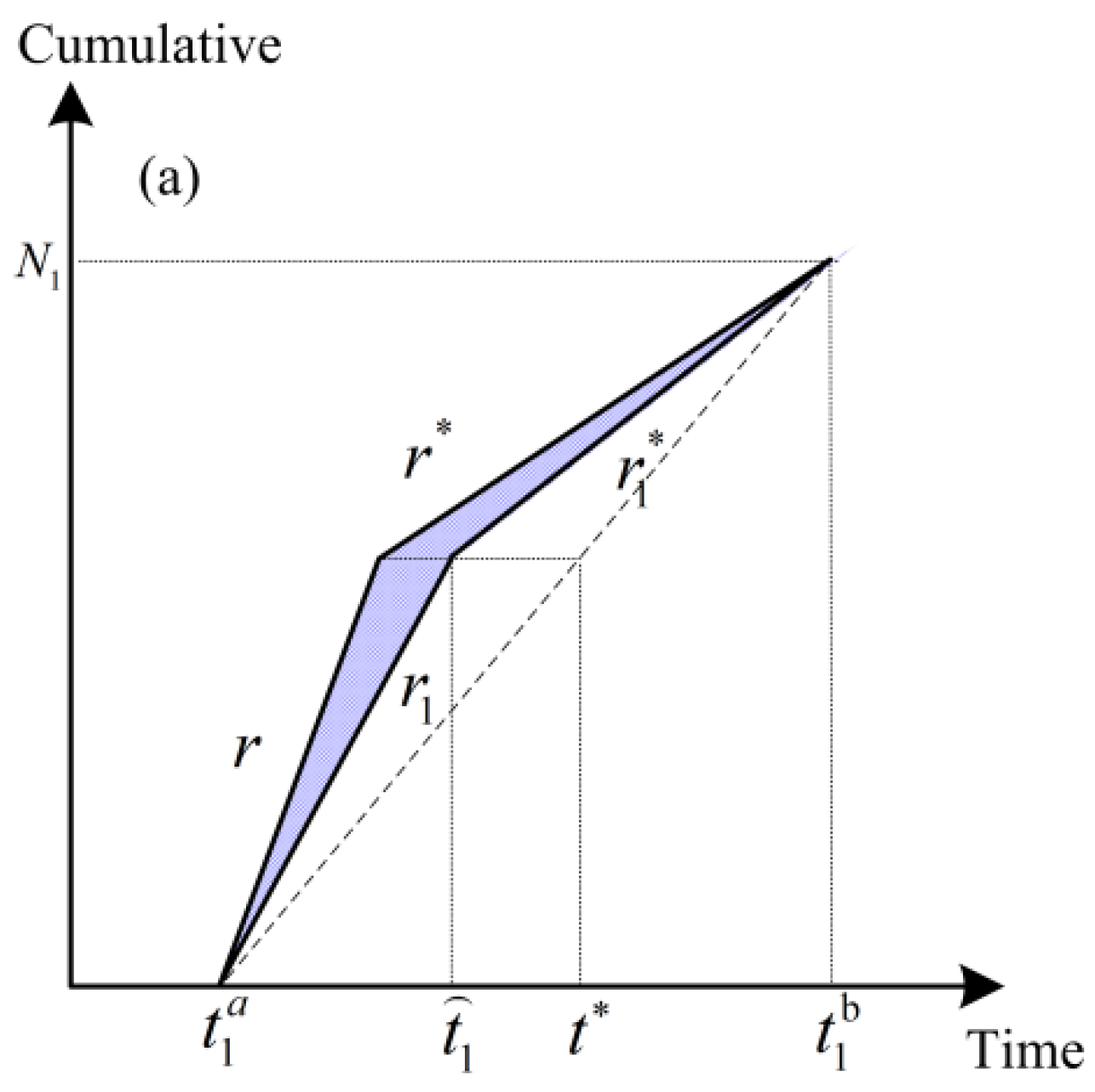
3.1. Pattern 1: Departure Equilibrium Pattern with Only SDs

As analyzed above, there are only SDs including in the commuting system when $\omega =0$. And Equation (5) show that the SD’s travel cost will not be affected by bottleneck location, we donate $t_1^a$, $t_1^b$ as the earliest and latest departure time for SD commuters, respectively. Let ${\stackrel{⌢}{t}}_1$ be the departure time of SD commuters who arrive at CBD on time. Differentiating Equation (5) with respect to $t$ and setting to zero, $d{c}_1(t)/dt=0$, the equilibrium departure rate from home for SD who arrive at the CBD before and after desired arrival time $t^{*}$, respectively, are given by

$$r_s=\{\begin{array}{c}{r}_1(t)=\frac{\alpha +g}{\alpha +g-\beta }\cdot s,\begin{array}{cc}& t\in (t_1^a,t^{*})\end{array}\\ r_1^{*}(t)=\frac{\alpha +g}{\alpha +g+\gamma }\cdot s\begin{array}{cc}& t\in (t^{*},t_1^b)\end{array}\end{array}$$

(7)

As shown in Figure 2, the departure rate $r_s$ is lower for early arrivals and higher for late arrivals than that obtained using the traditional bottleneck model when a time-dependent fuel cost is considered.

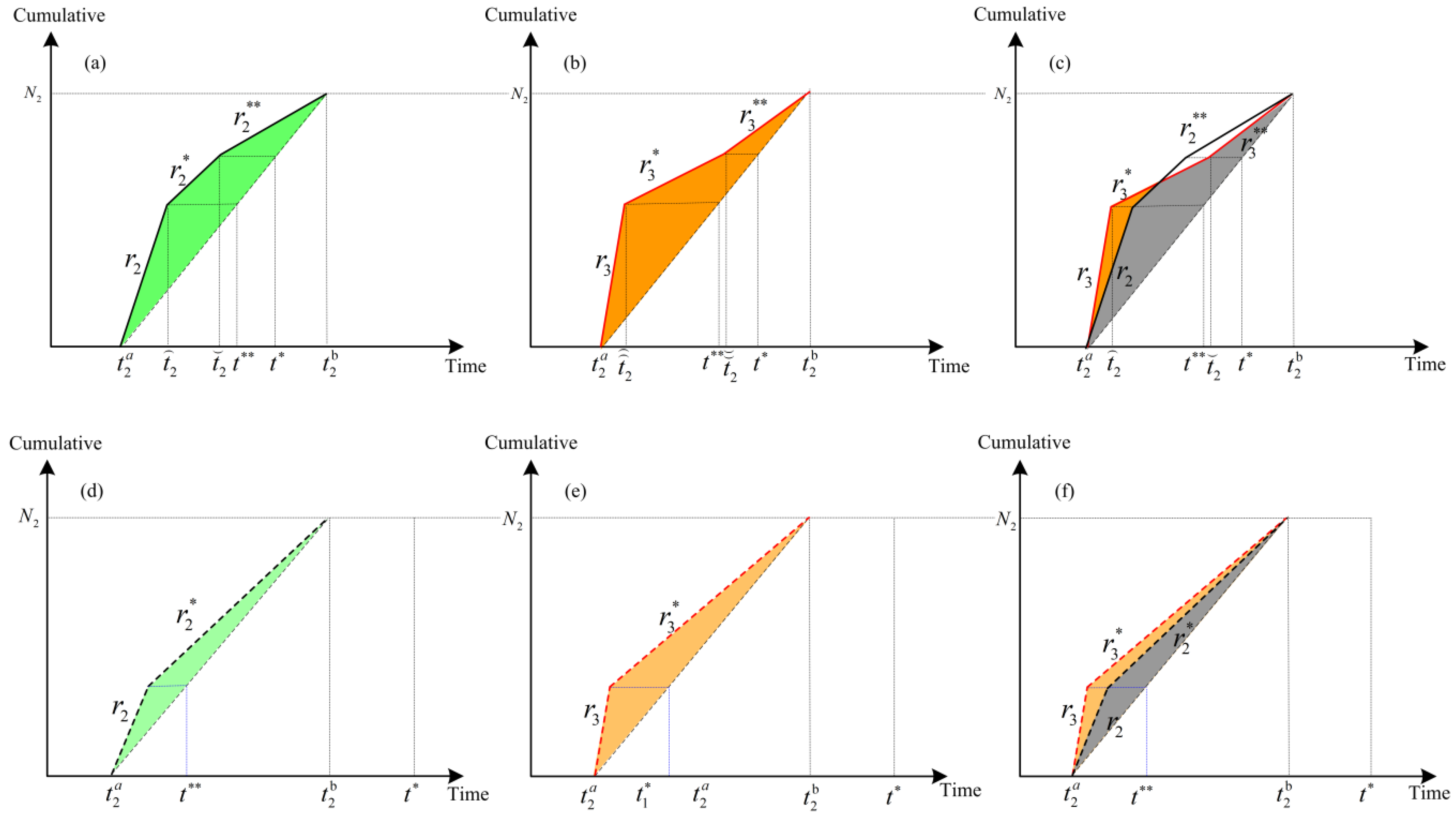
3.2. Pattern2: Departure Pattern of DUE with Only RDs

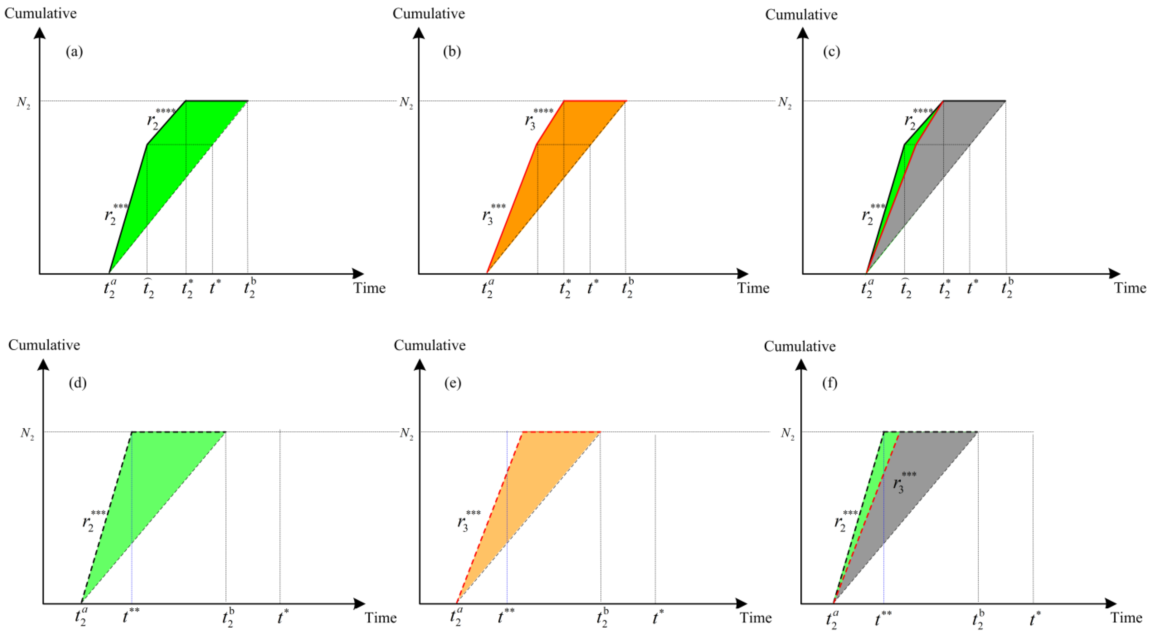
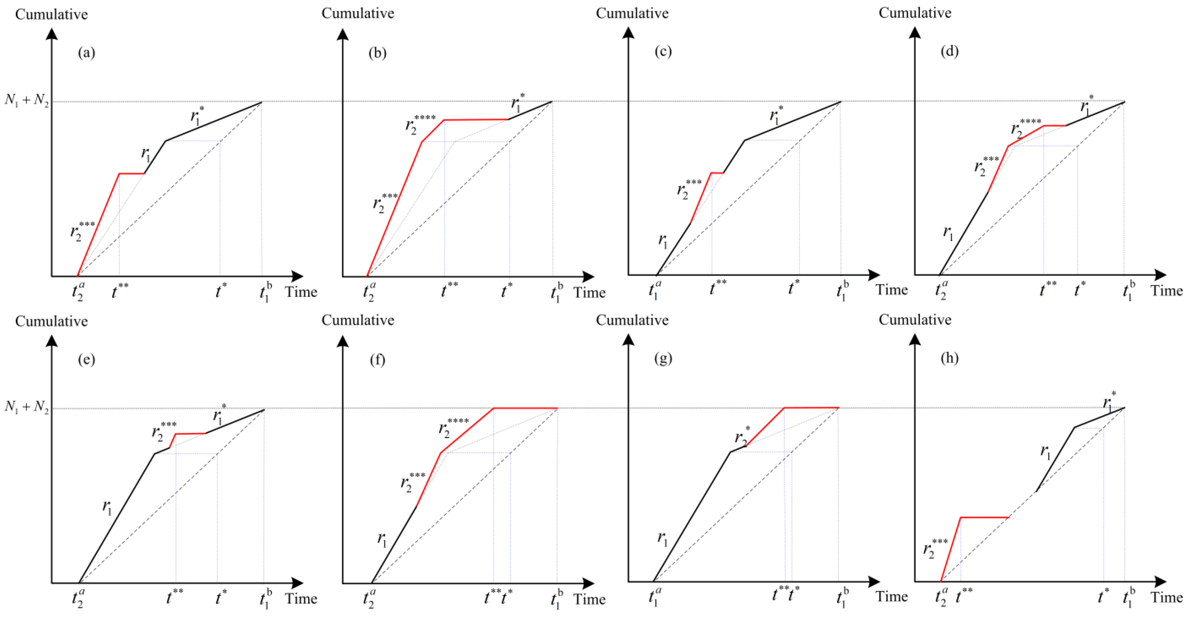
3.2.1. Departure Pattern of DUE with Only EDs in Cases of Pre-PC

The Pattern 2 will occur when $\omega =1$, in which only RDs driving on commuting corridor. In general, when the morning commute system achieves DUE stage, the different scenarios between Pre-PC and Post-PC lead to four diverse cost patterns for ridesharing participants: both early for pickup and work (Case 1), late for pickup but early for work (Case 2), early for pickup but late for work (Case 3), and both late for pickup and work (Case 4).

But the specific case is different when meeting different scenarios of Pre-PC or Post-PC. RDs will face three traffic cases (the Case 3 are not included) when they achieve user equilibrium if the bottleneck forms before pickup time. Unlike the case in Pre-PC, RD can avoid lateness penalty under the controllable trip time between the home and pickup place when the bottleneck develops behind the pickup point, because the free flow time is regarded as zero in the assumption above, they can be on time or early at desire pickup time, $t^{**}$, to reduce the cost of the queuing delay between the pickup place and destination. So, the morning commute of ridesharing participants will face two scenarios: one, both early for pickup and work (Case 1), and another early for pickup but late for work (Case 3).

Let $t_2^a$ be the start time of the earliest RD commuters, $t_2^b$ be the departure time of the latest RD commuters, and donate ${\stackrel{⌢}{t}}_2,$ ${\stackrel{⌣}{t}}_2$ be the departure time of RD commuters who arrive at pickup place and CBD on time, respectively. Combining Equations (6) and (8), and differentiating Equation (6) with respect to $t$ and setting to zero, $d{c}_2(t)/dt=0$, the equilibrium departure rate from home for pickup and work in scenarios of Pre-PC are given by:

$$r_d=\{\begin{array}{ll}{r}_2(t)=\frac{\alpha +g}{\alpha +g-2\beta }\cdot s\hfill & t\in (t_2^a,{\stackrel{⌢}{t}}_2)\hspace{0.17em}\hspace{0.17em}\mathrm{and}\hspace{0.17em}{T}_2(t)=0\hfill \\ r_2^{*}(t)=\frac{\alpha +g}{\alpha +g-\beta +\gamma }\cdot s\hfill & t\in ({\stackrel{⌢}{t}}_2,{\stackrel{⌣}{t}}_2)\hspace{0.17em}\hspace{0.17em}\mathrm{and}\hspace{0.17em}{T}_2(t)=0\hfill \\ r_2^{**}(t)=\frac{\alpha +g}{\alpha +g+2\gamma }\cdot s\hfill & t\in ({\stackrel{⌣}{t}}_2,t_2^b)\hspace{0.17em}\hspace{0.17em}\mathrm{and}\hspace{0.17em}{T}_2(t)=0\hfill \end{array}$$

(8)

where $r_d$, $r_d^{*}$ is the departure rate of ridesharing driver when meet the Pre-PC or the Post-PC respectively. As mentioned, $r_2(t)$, $r_2^{*}(t)$, $r_2^{**}(t)$ is the equilibrium departure rate in Pre-PC scenario at time $t$ for RDs with three traffic pattern: early for pick up and work, early for pick up but late for work and late for pick up and work, respectively, which can be shown in Figure 3a. Meanwhile, the departure rates $r_2^{***}$, $r_2^{****}$ of RDs in two case of Post-PC scenario are expressed in Figure 4, which represent Case 1 and Case 3, respectively.

The advances in mobile communication technologies (e.g., GPS location technology) not only help ridesharing drivers obtain the maximum utilities but also decrease the dynamic waiting time for passenger’s street-hailing, which have made sharing system easier and more efficient. Let $t_3^a$ be the start time of the earliest RP commuters, $t_3^b$ be the departure time of the latest RP commuters, and donate ${\stackrel{⌢}{t}}_3,$ ${\stackrel{⌣}{t}}_3$ be the departure time of RP commuters who match RDs at pickup place and CBD on time, respectively. Similarly, by combining and differentiating for Equations (7) and (8), the departure rate of RPs, $r_p$, $r_p^{*}$, who travel together from the pickup place to CBD ahead or behind the bottleneck respectively can be given as below:

$$r_p=\{\begin{array}{ll}{r}_3(t)=\frac{\alpha }{\alpha -2\beta }\cdot s& t\in (t_3^a,{\stackrel{⌢}{t}}_2)\hspace{0.17em}\hspace{0.17em}\mathrm{and}\hspace{0.17em}{T}_2(t)=0\\ r_3^{*}(t)=\frac{\alpha }{\alpha -\beta +\gamma }\cdot s& t\in (\stackrel{⌢}{t},{\stackrel{⌣}{t}}_2)\hspace{0.17em}\hspace{0.17em}\mathrm{and}\hspace{0.17em}{T}_2(t)=0\\ r_3^{**}(t)=\frac{\alpha }{\alpha +2\gamma }\cdot s& t\in ({\stackrel{⌣}{t}}_2,t_3^b)\hspace{0.17em}\hspace{0.17em}\mathrm{and}\hspace{0.17em}{T}_2(t)=0\end{array}$$

(9)

Details of the department rate of different scenarios are shown in

Table 1. Detail of department rate of different scenarios.

Scenarios		Bottleneck before Pickup			Bottleneck after Pickup
Extra cost		Departure rate
Time window		$t\in (t_1^a,t^{*})$	$t\in (t^{*},t_1^b)$		$t\in (t_1^a,t^{*})$	$t\in (t^{*},t_1^b)$
Solo Driver	none	$\frac{\alpha }{\alpha -\beta }\cdot s$	$\frac{\alpha }{\alpha +\gamma }\cdot s$		$\frac{\alpha }{\alpha -\beta }\cdot s$	$\frac{\alpha }{\alpha +\gamma }\cdot s$
	gasoline	$\frac{{\alpha }_1}{{\alpha }_1-\beta }\cdot s$	$\frac{{\alpha }_1}{{\alpha }_1+\gamma }\cdot s$		$\frac{{\alpha }_1}{{\alpha }_1-\beta }\cdot s$	$\frac{{\alpha }_1}{{\alpha }_1+\gamma }\cdot s$
Time window		$t\in (t_2^a,{\stackrel{⌢}{t}}_2)$	$t\in ({\stackrel{⌢}{t}}_2,{\stackrel{⌣}{t}}_2)$	$t\in ({\stackrel{⌣}{t}}_2,t_2^b)$
Ridesharing Driver	Gasoline&Compensation	$\frac{{\alpha }_1}{{\alpha }_1-2\beta }\cdot s$	$\frac{{\alpha }_1}{{\alpha }_1-\beta +\gamma }\cdot s$	$\frac{{\alpha }_1}{{\alpha }_1+2\gamma }\cdot s$	$\frac{{\alpha }_2+\beta }{{\alpha }_2-\beta }\cdot s$	$\frac{{\alpha }_2+\beta }{{\alpha }_2+\gamma }\cdot s$
Ridesharing Passenger	payment	$\frac{\alpha }{\alpha -2\beta }\cdot s$	$\frac{\alpha }{\alpha -\beta +\gamma }\cdot s$	$\frac{\alpha }{\alpha +2\gamma }\cdot s$	$\frac{{\alpha }_3+\beta }{{\alpha }_3-\beta }\cdot s$	$\frac{{\alpha }_3+\beta }{{\alpha }_3+\gamma }\cdot s$
Considering simplicity of analysis, let ${\alpha }_1=\alpha +g$, ${\alpha }_2=\alpha +g-\xi$, ${\alpha }_3=\alpha +\xi$

, and we can easily obtain the relationship among different scenarios: It yields $r_3>r_2>r_1>s>r_2^{*}>r_3^{*}>r_3^{**}>r_2^{**}>r_1^{*}$, $r_2^{***}>r_3^{***}>r_1>s>r_3^{****}>r_1^{*}>r_2^{****}$ in Pre-PC and Post-PC patterns, respectively.

3.2.2. Departure Pattern of DUE with Only EDs in Different PW Schedule Gap

In this section, we will consider the different equilibrium traffic scenarios that may occur in reality with the formulations in Section 3.1 and Section 3.2. Depending on the pickup-work (PW) schedule gap, $\Delta t=t^{\ast }-t^{\ast \ast }$, there are two possible case that may arise at equilibrium. If $\Delta t=t^{\ast }-t^{\ast \ast }$ is extremely smaller, there will be some ridesharing participants who arrive later than the desired work time no matter in Pre-PC or Post-PC scenario when morning commute system achieves equilibrium, which means RDs and RPs may depart from home in case 1, 2, and 4 under Pre-PC condition (the right side in Figure 3a–c), and in case 1 and 3 under Post-PC condition (the right side in Figure 4d–f), respectively. The same occurs as if $\Delta t=t^{\ast }-t^{\ast \ast }$ is extremely larger, all ridesharing participants will arrive later than the desired work time, regardless of Pre-PC or Post-PC scenario when the morning commute system achieves equilibrium, which means RDs and RPs depart from home only in Case 1 and 2 under Pre-PC condition, which are shown as dotted part (left side) in Figure 3a–c and they may depart from home only in case 1 under Post-PC condition, which are shown as dotted part (left side) in Figure 4a–c.

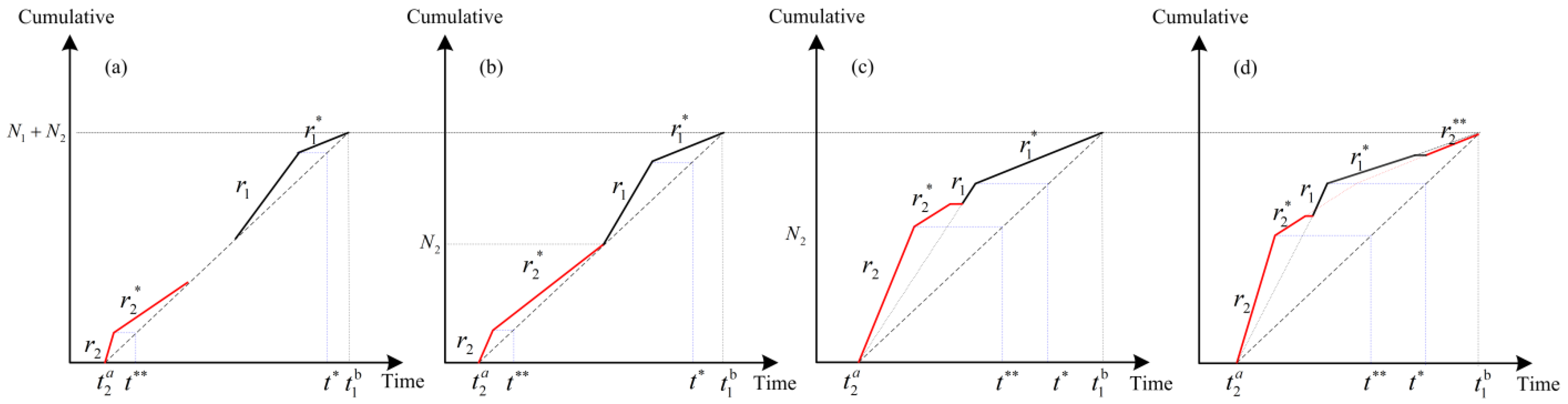
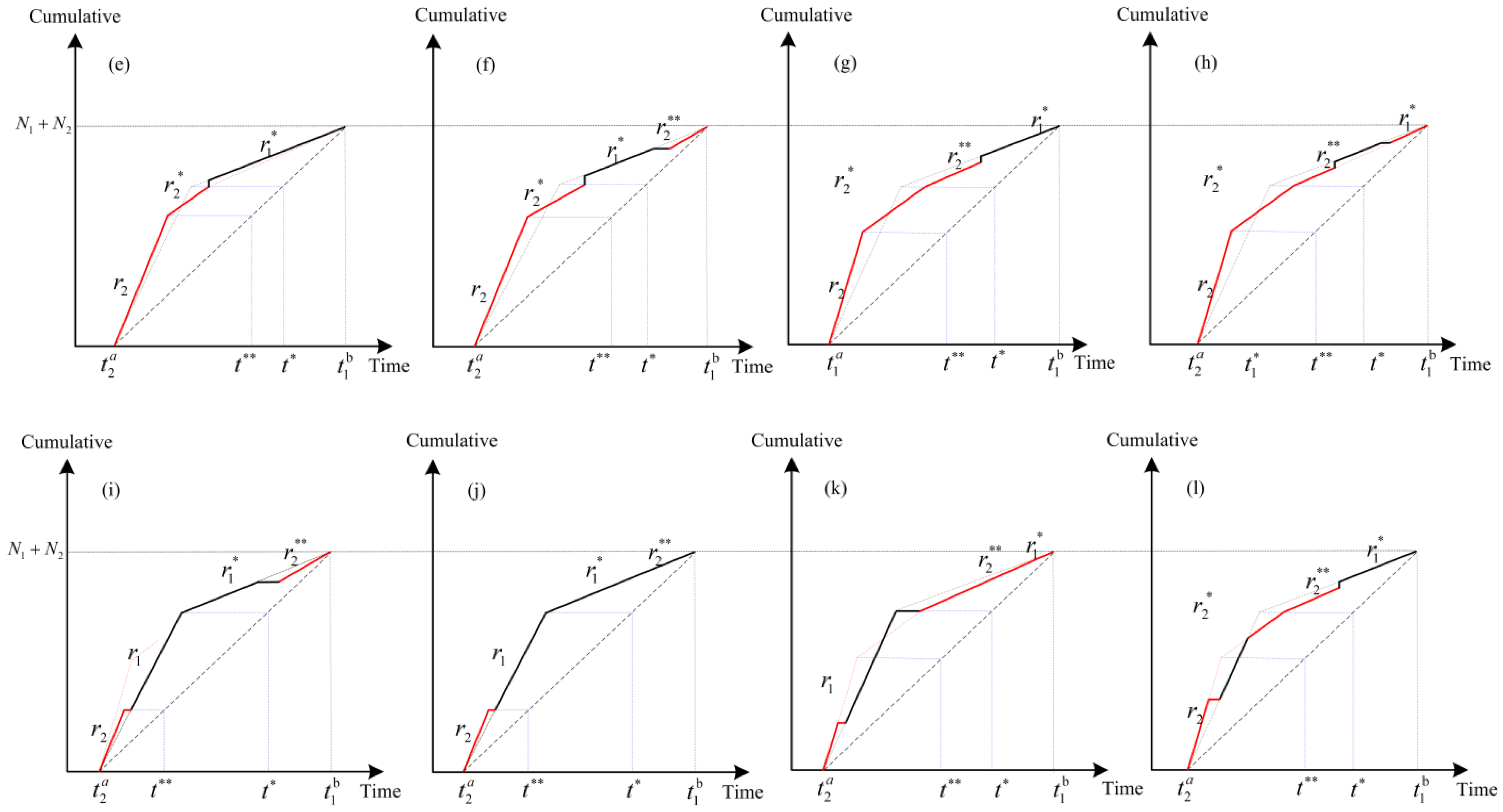
4. Departure Patterns of DUE with Mixed Commuters

4.1. Single-Peaked and Double-Peaked Cases of DUE with Mixed Commuters

In this section, the mixed scenario with SDs and RDs under uncertain bottleneck condition is examined according to two important parameter variables: the PW schedule gap, $\Delta t$ and proportion of mixed commuters, $N_1/N_2$, which is expressed by Equation (12) and Equation (13), respectively.

$$\Delta t=t^{\ast }-t^{\ast \ast }=\frac{\gamma }{\beta +\gamma }\frac{N_1}{s}+\frac{2\beta }{\beta +\gamma }\frac{N_2}{s}-\mu$$

(10)

$$\frac{N_1}{N_2}=\frac{\beta }{\gamma }-\rho$$

(11)

where $\mu \hspace{0.17em}(\mu \ge 0)$ is a concept of the staggered coefficient according to the theory of staggered shifts theory, it can be used to determine the sufficient and necessary condition for the existence of the double-peaked and single-peaked queue in MCS under uncertain bottleneck scenarios. Meanwhile, $\rho$ is a parameter for proportion of mixed commuters, $N_1/N_2$. We can confirm that $N_1/N_2>\beta /\gamma$, when $\rho <0$; $N_1/N_2<\beta /\gamma$, when $\rho >0$ and $N_1/N_2=\beta /\gamma$, when $\rho =0$.

All possible DUE traffic patterns under Pre-PC situation are shown in Figure 5, other potential ones under Post-PC situation are shown in Figure 6. Note that departure curves of DUE for RDs and SDs are represented by red line and black lines in both Figure 5 and Figure 6, respectively.

Figure 5a–h display the different DUE patterns of double-peaked queuing under Pre-PC, while Figure 5i–l delineate the different DUE pattern of single-peaked queuing under Pre-PC. By the way, considering ridesharing passenger waiting willingness, the cases in Figure 5d,f,h,I,k,l rarely happen in reality. Moreover, the optimal punctual time gap $\Delta t^{\ast }$ of system in Pre-PC and Post-PC are also displayed in Figure 5b and Figure 6a, respectively.

By contrast, Figure 6a,b,h illustrate the different DUE pattern of double-peaked queuing under Post-PC, while Figure 6c–g show the different DUE pattern of single-peaked queuing under Post-PC.

4.2. User Equilibrium and System Optimal

In this section, we show all possible commuting patterns, now we examine the user’s travel costs under double-peaked queuing case and single-peaked queuing case. Based on the equilibrium commuting scenarios of Figure 5 and Figure 6, we can obtain the trip cost of SDs and RDs under DUE stage, for Pre-PC pattern (when $N_1/N_2>\frac{\beta }{\gamma }$):

$$c_1=\{\begin{array}{cc}\frac{\beta \gamma }{\beta +\gamma }\frac{N_1}{s},\hspace{0.17em}\hspace{0.17em}\hspace{0.17em}\hspace{0.17em}\hspace{0.17em}\hspace{0.17em}\hspace{0.17em}\hspace{0.17em}\hspace{0.17em}\hspace{0.17em}\hspace{0.17em}\hspace{0.17em}\hspace{0.17em}\hspace{0.17em}\hspace{0.17em}\hspace{0.17em}\hspace{0.17em}\hspace{0.17em}\hspace{0.17em}\hspace{0.17em}\hspace{0.17em}\hfill & \Delta t\le \Delta t^{\ast }-\max \left\{\frac{2\beta }{\beta +\gamma }\frac{N_1}{s},\frac{2\gamma }{\beta +\gamma }\frac{N_2}{s}\right\}\\ \frac{1}{2}\frac{\beta \gamma }{\beta +\gamma }\frac{N}{s}+\frac{\beta }{2}\frac{N_1}{s}-\frac{1}{2}\gamma \Delta t,\hfill & \Delta t^{\ast }-\max \left\{\frac{2\beta }{\beta +\gamma }\frac{N_1}{s},\frac{2\gamma }{\beta +\gamma }\frac{N_2}{s}\right\}<\Delta t\le \Delta t^{\ast }\\ \frac{\beta \gamma }{\beta +\gamma }\frac{N}{s},\hspace{0.17em}\hspace{0.17em}\hspace{0.17em}\hspace{0.17em}\hspace{0.17em}\hspace{0.17em}\hspace{0.17em}\hspace{0.17em}\hspace{0.17em}\hspace{0.17em}\hspace{0.17em}\hspace{0.17em}\hspace{0.17em}\hspace{0.17em}\hspace{0.17em}\hspace{0.17em}\hspace{0.17em}\hspace{0.17em}\hspace{0.17em}\hspace{0.17em}\hspace{0.17em}\hspace{0.17em}\hfill & \Delta t\ge \Delta t^{\ast }\end{array}$$

(12)

$$c_2=\{\begin{array}{cc}\frac{2\beta \gamma }{\beta +\gamma }\frac{N}{s}-\beta \Delta t,\hspace{0.17em}\hspace{0.17em}\hspace{0.17em}\hspace{0.17em}\hspace{0.17em}\hspace{0.17em}\hspace{0.17em}\hspace{0.17em}\hspace{0.17em}\hspace{0.17em}\hspace{0.17em}\hspace{0.17em}\hspace{0.17em}\hspace{0.17em}\hspace{0.17em}\hfill & \Delta t\le \Delta t^{\ast }-\max \left\{\frac{2\beta }{\beta +\gamma }\frac{N_1}{s},\frac{2\gamma }{\beta +\gamma }\frac{N_2}{s}\right\}\\ \frac{1}{2}\frac{\beta \gamma }{\beta +\gamma }\frac{N}{s}+\frac{\beta }{2}\frac{N_1}{s}-\frac{1}{2}\beta \Delta t,\hfill & \Delta t^{\ast }-\max \left\{\frac{2\beta }{\beta +\gamma }\frac{N_1}{s},\frac{2\gamma }{\beta +\gamma }\frac{N_2}{s}\right\}<\Delta t\le \Delta t^{\ast }\\ \frac{2\beta \gamma }{\beta +\gamma }\frac{N_2}{s}+\beta \Delta t\hspace{0.17em}\hspace{0.17em}\hspace{0.17em}\hspace{0.17em}\hspace{0.17em}\hspace{0.17em}\hspace{0.17em}\hspace{0.17em}\hspace{0.17em}\hspace{0.17em}\hspace{0.17em}\hspace{0.17em}\hspace{0.17em}\hspace{0.17em}\hspace{0.17em}\hspace{0.17em}\hspace{0.17em}\hfill & \Delta t\ge \Delta t^{\ast }\end{array}$$

(13)

For Pre-PC pattern (when $N_1/N_2<\frac{\beta }{\gamma }$):

$$c_1=\{\begin{array}{cc}\frac{\beta \gamma }{\beta +\gamma }\frac{N_1}{s},\hspace{0.17em}\hspace{0.17em}\hspace{0.17em}\hspace{0.17em}\hspace{0.17em}\hspace{0.17em}\hspace{0.17em}\hspace{0.17em}\hspace{0.17em}\hspace{0.17em}\hspace{0.17em}\hspace{0.17em}\hspace{0.17em}\hspace{0.17em}\hspace{0.17em}\hspace{0.17em}\hspace{0.17em}\hspace{0.17em}\hspace{0.17em}\hspace{0.17em}\hspace{0.17em}\hspace{0.17em}\hspace{0.17em}\hspace{0.17em}\hspace{0.17em}\hfill & \Delta t\le \Delta t^{\ast }-\max \left\{\frac{2\beta }{\beta +\gamma }\frac{N_1}{s},\frac{2\gamma }{\beta +\gamma }\frac{N_2}{s}\right\}\\ \frac{1}{2}\frac{\beta \gamma }{\beta +\gamma }\frac{N}{s}-\frac{1}{2}\gamma \Delta t,\hspace{0.17em}\hspace{0.17em}\hspace{0.17em}\hspace{0.17em}\hspace{0.17em}\hspace{0.17em}\hspace{0.17em}\hspace{0.17em}\hspace{0.17em}\hspace{0.17em}\hspace{0.17em}\hspace{0.17em}\hspace{0.17em}\hspace{0.17em}\hfill & \Delta t^{\ast }-\max \left\{\frac{2\beta }{\beta +\gamma }\frac{N_1}{s},\frac{2\gamma }{\beta +\gamma }\frac{N_2}{s}\right\}<\Delta t\le \Delta t^{\ast }\\ \frac{\beta \gamma }{\beta +\gamma }\frac{N}{s},\hspace{0.17em}\hspace{0.17em}\hspace{0.17em}\hspace{0.17em}\hspace{0.17em}\hspace{0.17em}\hspace{0.17em}\hspace{0.17em}\hspace{0.17em}\hspace{0.17em}\hspace{0.17em}\hspace{0.17em}\hspace{0.17em}\hspace{0.17em}\hspace{0.17em}\hspace{0.17em}\hspace{0.17em}\hspace{0.17em}\hspace{0.17em}\hspace{0.17em}\hspace{0.17em}\hspace{0.17em}\hspace{0.17em}\hspace{0.17em}\hspace{0.17em}\hfill & \Delta t\ge \Delta t^{\ast }\end{array}$$

(14)

$$c_2=\{\begin{array}{cc}\frac{2\beta \gamma }{\beta +\gamma }\frac{N}{s}-\beta \Delta t,\hspace{0.17em}\hspace{0.17em}\hspace{0.17em}\hspace{0.17em}\hspace{0.17em}\hspace{0.17em}\hspace{0.17em}\hspace{0.17em}\hspace{0.17em}\hspace{0.17em}\hspace{0.17em}\hspace{0.17em}\hspace{0.17em}\hspace{0.17em}\hspace{0.17em}\hspace{0.17em}\hspace{0.17em}\hspace{0.17em}\hspace{0.17em}\hspace{0.17em}\hspace{0.17em}\hfill & \Delta t\le \Delta t^{\ast }-\max \left\{\frac{2\beta }{\beta +\gamma }\frac{N_1}{s},\frac{2\gamma }{\beta +\gamma }\frac{N_2}{s}\right\}\\ \frac{2\beta \gamma }{\beta +\gamma }\frac{N}{s},\hspace{0.17em}\hspace{0.17em}\hspace{0.17em}\hspace{0.17em}\hspace{0.17em}\hspace{0.17em}\hspace{0.17em}\hspace{0.17em}\hspace{0.17em}\hspace{0.17em}\hspace{0.17em}\hspace{0.17em}\hspace{0.17em}\hspace{0.17em}\hspace{0.17em}\hspace{0.17em}\hspace{0.17em}\hspace{0.17em}\hspace{0.17em}\hspace{0.17em}\hspace{0.17em}\hspace{0.17em}\hspace{0.17em}\hspace{0.17em}\hspace{0.17em}\hspace{0.17em}\hspace{0.17em}\hspace{0.17em}\hspace{0.17em}\hfill & \Delta t^{\ast }-\max \left\{\frac{2\beta }{\beta +\gamma }\frac{N_1}{s},\frac{2\gamma }{\beta +\gamma }\frac{N_2}{s}\right\}<\Delta t\le \Delta t^{\ast }\\ \frac{\beta \gamma }{\beta +\gamma }\frac{N_2}{s}+\beta \Delta t,\hspace{0.17em}\hspace{0.17em}\hspace{0.17em}\hspace{0.17em}\hspace{0.17em}\hspace{0.17em}\hspace{0.17em}\hspace{0.17em}\hspace{0.17em}\hspace{0.17em}\hspace{0.17em}\hspace{0.17em}\hspace{0.17em}\hspace{0.17em}\hspace{0.17em}\hspace{0.17em}\hspace{0.17em}\hspace{0.17em}\hspace{0.17em}\hspace{0.17em}\hfill & \Delta t\ge \Delta t^{\ast }\end{array}$$

(15)

where $\Delta t^{\ast }=\frac{\gamma }{\beta +\gamma }\frac{N_1}{s}+\frac{2\beta }{\beta +\gamma }\frac{N_2}{s}$, for given $\Delta t=t^{\ast }-t^{\ast \ast }$, the queuing of morning commute system with SDs changes from single-peaked case to double-peaked case with $\Delta t$. Equation (13) indicates that the trip cost of RDs is decreasing with $\Delta t$ when $\Delta t\le \Delta t^{\ast }$ and the number of RDs is small ($N_1/N_2>\frac{\beta }{\gamma }$), and then increasing with $\Delta t$, here two groups of commuters depart separately without interaction. In stark contrast, Equation (12) displays that the trip cost of SDs will retain fixation in single-peaked case with $\Delta t$ when $\Delta t\le \Delta t^{\ast }$ and the number of RDs is small ($N_1/N_2>\frac{\beta }{\gamma }$), then the trip cost is decreasing with $\Delta t$ in double-peaked case when $\Delta t^{\ast }-\max \left\{\frac{2\beta }{\beta +\gamma }\frac{N_1}{s},\frac{2\gamma }{\beta +\gamma }\frac{N_2}{s}\right\}<\Delta t\le \Delta t^{\ast }$. And then maintain fixed cost when $\Delta t\ge \Delta t^{\ast }$. And when the number of RDs is large ($N_1/N_2<\frac{\beta }{\gamma }$) in the Pre-PC pattern, RDs meet the similar cost case whose queuing behavior of EU is single-peaked, while RDs have a fixed cost when meet double-peaked queuing, which is different from whose case in $N_1/N_2<\frac{\beta }{\gamma }$.

For Post-PC pattern: (when $N_1/N_2>\frac{\beta }{\gamma }$)

$${c^{\prime }}_1=\{\begin{array}{cc}\frac{\beta ({\alpha }_1+\gamma )}{{\alpha }_1+\beta +\gamma }\frac{N_1}{s}+\frac{\beta ({\alpha }_1+\gamma )}{{\alpha }_1+\beta +\gamma }\cdot \frac{{\alpha }_1+\gamma }{{\alpha }_1+\beta }\frac{N_2}{s}+\frac{{\alpha }_1\beta }{{\alpha }_1+\beta +\gamma }\Delta t,\hfill & \Delta t\le \Delta t^{\ast }-\max \left\{\frac{2\beta }{\beta +\gamma }\frac{N_1}{s},\frac{2\gamma }{\beta +\gamma }\frac{N_2}{s}\right\}\\ \frac{\beta \gamma }{\beta +\gamma }\frac{N}{s},\hspace{0.17em}\hspace{0.17em}\hspace{0.17em}\hspace{0.17em}\hspace{0.17em}\hspace{0.17em}\hspace{0.17em}\hspace{0.17em}\hspace{0.17em}\hspace{0.17em}\hspace{0.17em}\hspace{0.17em}\hspace{0.17em}\hspace{0.17em}\hspace{0.17em}\hspace{0.17em}\hspace{0.17em}\hspace{0.17em}\hspace{0.17em}\hspace{0.17em}\hspace{0.17em}\hspace{0.17em}\hspace{0.17em}\hspace{0.17em}\hspace{0.17em}\hspace{0.17em}\hspace{0.17em}\hspace{0.17em}\hspace{0.17em}\hspace{0.17em}\hspace{0.17em}\hspace{0.17em}\hspace{0.17em}\hspace{0.17em}\hspace{0.17em}\hspace{0.17em}\hspace{0.17em}\hspace{0.17em}\hspace{0.17em}\hspace{0.17em}\hspace{0.17em}\hspace{0.17em}\hspace{0.17em}\hspace{0.17em}\hspace{0.17em}\hspace{0.17em}\hspace{0.17em}\hspace{0.17em}\hspace{0.17em}\hspace{0.17em}\hspace{0.17em}\hspace{0.17em}\hspace{0.17em}\hspace{0.17em}\hspace{0.17em}\hspace{0.17em}\hspace{0.17em}\hspace{0.17em}\hspace{0.17em}\hfill & \Delta t^{\ast }-\max \left\{\frac{2\beta }{\beta +\gamma }\frac{N_1}{s},\frac{2\gamma }{\beta +\gamma }\frac{N_2}{s}\right\}<\Delta t\le \Delta t^{\ast }\\ \frac{\beta \gamma }{\beta +\gamma }\frac{N_1}{s},\hspace{0.17em}\hspace{0.17em}\hspace{0.17em}\hspace{0.17em}\hspace{0.17em}\hspace{0.17em}\hspace{0.17em}\hspace{0.17em}\hspace{0.17em}\hspace{0.17em}\hspace{0.17em}\hspace{0.17em}\hspace{0.17em}\hspace{0.17em}\hspace{0.17em}\hspace{0.17em}\hspace{0.17em}\hspace{0.17em}\hspace{0.17em}\hspace{0.17em}\hspace{0.17em}\hspace{0.17em}\hspace{0.17em}\hspace{0.17em}\hspace{0.17em}\hspace{0.17em}\hspace{0.17em}\hspace{0.17em}\hspace{0.17em}\hspace{0.17em}\hspace{0.17em}\hspace{0.17em}\hspace{0.17em}\hspace{0.17em}\hspace{0.17em}\hspace{0.17em}\hspace{0.17em}\hspace{0.17em}\hspace{0.17em}\hspace{0.17em}\hspace{0.17em}\hspace{0.17em}\hspace{0.17em}\hspace{0.17em}\hspace{0.17em}\hspace{0.17em}\hspace{0.17em}\hspace{0.17em}\hspace{0.17em}\hspace{0.17em}\hspace{0.17em}\hspace{0.17em}\hspace{0.17em}\hspace{0.17em}\hspace{0.17em}\hspace{0.17em}\hspace{0.17em}\hspace{0.17em}\hfill & \Delta t\ge \Delta t^{\ast }\end{array}$$

(16)

$${c^{\prime }}_2=\{\begin{array}{cc}\frac{\beta ({\alpha }_1+\gamma )}{{\alpha }_1+\beta +\gamma }\frac{N_1}{s}+\frac{\beta ({\alpha }_1+\gamma )}{{\alpha }_1+\beta +\gamma }(1+\frac{{\alpha }_1+\gamma }{{\alpha }_1+\beta })\frac{N_2}{s}+\frac{{\alpha }_1\beta }{{\alpha }_1+\beta +\gamma }\Delta t,\hfill & \Delta t\le \Delta t^{\ast }-\max \left\{\frac{2\beta }{\beta +\gamma }\frac{N_1}{s},\frac{2\gamma }{\beta +\gamma }\frac{N_2}{s}\right\}\\ \frac{\beta \gamma }{\beta +\gamma }\frac{N_1}{s}+(\frac{\beta \gamma }{\beta +\gamma }+\frac{\beta (\alpha -\beta )}{\alpha +\beta })\frac{N_2}{s},\hspace{0.17em}\hspace{0.17em}\hspace{0.17em}\hspace{0.17em}\hspace{0.17em}\hspace{0.17em}\hspace{0.17em}\hspace{0.17em}\hspace{0.17em}\hspace{0.17em}\hspace{0.17em}\hspace{0.17em}\hspace{0.17em}\hspace{0.17em}\hspace{0.17em}\hspace{0.17em}\hspace{0.17em}\hspace{0.17em}\hspace{0.17em}\hspace{0.17em}\hspace{0.17em}\hspace{0.17em}\hspace{0.17em}\hspace{0.17em}\hspace{0.17em}\hspace{0.17em}\hspace{0.17em}\hfill & \Delta t^{\ast }-\max \left\{\frac{2\beta }{\beta +\gamma }\frac{N_1}{s},\frac{2\gamma }{\beta +\gamma }\frac{N_2}{s}\right\}<\Delta t\le \Delta t^{\ast }\\ \frac{2\beta ({\alpha }_1-\beta )}{{\alpha }_1+\beta }\frac{N_2}{s}+\beta \Delta t,\hspace{0.17em}\hspace{0.17em}\hspace{0.17em}\hspace{0.17em}\hspace{0.17em}\hspace{0.17em}\hspace{0.17em}\hspace{0.17em}\hspace{0.17em}\hspace{0.17em}\hspace{0.17em}\hspace{0.17em}\hspace{0.17em}\hspace{0.17em}\hspace{0.17em}\hspace{0.17em}\hspace{0.17em}\hspace{0.17em}\hspace{0.17em}\hspace{0.17em}\hspace{0.17em}\hspace{0.17em}\hspace{0.17em}\hspace{0.17em}\hspace{0.17em}\hspace{0.17em}\hspace{0.17em}\hspace{0.17em}\hspace{0.17em}\hspace{0.17em}\hspace{0.17em}\hspace{0.17em}\hspace{0.17em}\hspace{0.17em}\hspace{0.17em}\hspace{0.17em}\hspace{0.17em}\hspace{0.17em}\hspace{0.17em}\hspace{0.17em}\hspace{0.17em}\hspace{0.17em}\hspace{0.17em}\hspace{0.17em}\hspace{0.17em}\hspace{0.17em}\hfill & \Delta t\ge \Delta t^{\ast }\end{array}$$

(17)

For Post-PC pattern: (when $N_1/N_2<\frac{\beta }{\gamma }$)

$${c^{\prime }}_1=\{\begin{array}{cc}\frac{\beta ({\alpha }_1+\gamma )}{{\alpha }_1+\beta +\gamma }\frac{N_1}{s}+\frac{\beta ({\alpha }_1+\gamma )}{{\alpha }_1+\beta +\gamma }\cdot \frac{{\alpha }_1+\gamma }{{\alpha }_1+\beta }\frac{N_2}{s}+\frac{{\alpha }_1\beta }{{\alpha }_1+\beta +\gamma }\Delta t,\hfill & \Delta t\le \Delta t^{\ast }-\max \left\{\frac{2\beta }{\beta +\gamma }\frac{N_1}{s},\frac{2\gamma }{\beta +\gamma }\frac{N_2}{s}\right\}\\ \gamma \frac{N_1}{s}+\frac{2\gamma \beta }{\alpha +2\beta +\gamma }\frac{N_2}{s}-\frac{\gamma ({\alpha }_1+\beta )}{{\alpha }_1+2\beta +\gamma }\Delta t,\hspace{0.17em}\hspace{0.17em}\hspace{0.17em}\hspace{0.17em}\hspace{0.17em}\hspace{0.17em}\hspace{0.17em}\hspace{0.17em}\hspace{0.17em}\hspace{0.17em}\hspace{0.17em}\hspace{0.17em}\hspace{0.17em}\hspace{0.17em}\hspace{0.17em}\hspace{0.17em}\hspace{0.17em}\hspace{0.17em}\hspace{0.17em}\hspace{0.17em}\hspace{0.17em}\hspace{0.17em}\hspace{0.17em}\hfill & \Delta t^{\ast }-\max \left\{\frac{2\beta }{\beta +\gamma }\frac{N_1}{s},\frac{2\gamma }{\beta +\gamma }\frac{N_2}{s}\right\}<\Delta t\le \Delta t^{\ast }\\ \frac{\beta \gamma }{\beta +\gamma }\frac{N_1}{s},\hspace{0.17em}\hspace{0.17em}\hspace{0.17em}\hspace{0.17em}\hspace{0.17em}\hspace{0.17em}\hspace{0.17em}\hspace{0.17em}\hspace{0.17em}\hspace{0.17em}\hspace{0.17em}\hspace{0.17em}\hspace{0.17em}\hspace{0.17em}\hspace{0.17em}\hspace{0.17em}\hspace{0.17em}\hspace{0.17em}\hspace{0.17em}\hspace{0.17em}\hspace{0.17em}\hspace{0.17em}\hspace{0.17em}\hspace{0.17em}\hspace{0.17em}\hspace{0.17em}\hspace{0.17em}\hspace{0.17em}\hspace{0.17em}\hspace{0.17em}\hspace{0.17em}\hspace{0.17em}\hspace{0.17em}\hspace{0.17em}\hspace{0.17em}\hspace{0.17em}\hspace{0.17em}\hspace{0.17em}\hspace{0.17em}\hspace{0.17em}\hspace{0.17em}\hspace{0.17em}\hspace{0.17em}\hspace{0.17em}\hspace{0.17em}\hspace{0.17em}\hspace{0.17em}\hspace{0.17em}\hspace{0.17em}\hspace{0.17em}\hspace{0.17em}\hspace{0.17em}\hspace{0.17em}\hspace{0.17em}\hspace{0.17em}\hspace{0.17em}\hspace{0.17em}\hspace{0.17em}\hspace{0.17em}\hspace{0.17em}\hspace{0.17em}\hfill & \Delta t\ge \Delta t^{\ast }\end{array}$$

(18)

$${c^{\prime }}_2=\{\begin{array}{cc}\frac{\beta ({\alpha }_1+\gamma )}{{\alpha }_1+\beta +\gamma }\frac{N_1}{s}+\frac{\beta ({\alpha }_1+\gamma )}{{\alpha }_1+\beta +\gamma }(1+\frac{{\alpha }_1+\gamma }{{\alpha }_1+\beta })\frac{N_2}{s}+\frac{{\alpha }_1\beta }{{\alpha }_1+\beta +\gamma }\Delta t,\hfill & \Delta t\le \Delta t^{\ast }-\max \left\{\frac{2\beta }{\beta +\gamma }\frac{N_1}{s},\frac{2\gamma }{\beta +\gamma }\frac{N_2}{s}\right\}\hfill \\ \frac{2\gamma \beta }{{\alpha }_1+2\beta +\gamma }\frac{N_2}{s}-\frac{\gamma ({\alpha }_1+\beta )}{{\alpha }_1+2\beta +\gamma }\Delta t,\hspace{0.17em}\hspace{0.17em}\hspace{0.17em}\hspace{0.17em}\hspace{0.17em}\hspace{0.17em}\hspace{0.17em}\hspace{0.17em}\hspace{0.17em}\hspace{0.17em}\hspace{0.17em}\hspace{0.17em}\hspace{0.17em}\hspace{0.17em}\hspace{0.17em}\hspace{0.17em}\hspace{0.17em}\hspace{0.17em}\hspace{0.17em}\hspace{0.17em}\hspace{0.17em}\hspace{0.17em}\hspace{0.17em}\hspace{0.17em}\hspace{0.17em}\hspace{0.17em}\hspace{0.17em}\hspace{0.17em}\hspace{0.17em}\hspace{0.17em}\hspace{0.17em}\hspace{0.17em}\hfill & \Delta t^{\ast }-\max \left\{\frac{2\beta }{\beta +\gamma }\frac{N_1}{s},\frac{2\gamma }{\beta +\gamma }\frac{N_2}{s}\right\}<\Delta t\le \Delta t^{\ast }\\ 2\beta \frac{{\alpha }_1-\beta }{{\alpha }_1+\beta }\frac{N_2}{s}+\beta \Delta t,\hspace{0.17em}\hspace{0.17em}\hspace{0.17em}\hspace{0.17em}\hspace{0.17em}\hspace{0.17em}\hspace{0.17em}\hspace{0.17em}\hspace{0.17em}\hspace{0.17em}\hspace{0.17em}\hspace{0.17em}\hspace{0.17em}\hspace{0.17em}\hspace{0.17em}\hspace{0.17em}\hspace{0.17em}\hspace{0.17em}\hspace{0.17em}\hspace{0.17em}\hspace{0.17em}\hspace{0.17em}\hspace{0.17em}\hspace{0.17em}\hspace{0.17em}\hspace{0.17em}\hspace{0.17em}\hspace{0.17em}\hspace{0.17em}\hspace{0.17em}\hspace{0.17em}\hspace{0.17em}\hspace{0.17em}\hspace{0.17em}\hspace{0.17em}\hspace{0.17em}\hspace{0.17em}\hspace{0.17em}\hspace{0.17em}\hspace{0.17em}\hspace{0.17em}\hspace{0.17em}\hspace{0.17em}\hspace{0.17em}\hspace{0.17em}\hspace{0.17em}\hspace{0.17em}& \Delta t\ge \Delta t^{\ast }\end{array}$$

(19)

Considering Equations (16)–(19) and a comparison between Figure 5 and Figure 6, we can know that some behaviour under user equilibrium changes because RDs don’t need to consider the effect of punctual pickup time when commuters meet the case of bottleneck occurring after pickup point. The travel cost of SDs shows the characteristics of dynamic change in the transition process between single-peaked queue and double-peaked queue, and then converges to a fixed value, while the travel cost of RDs indicates different functions in a double-peaked case among different domains of ($N_1,N_2$).

5. Conclusions

The aim of this paper is generally to analyse the ridesharing behavior in respect of the morning commuter problem considering different congestion patterns. Considering that the congested road bottleneck is uncertain, it can be separated into two patterns: pre-pickup congestion (Pre-PC) and post-pickup congestion (Post-PC). The analysis results of pickup-work trips and ridesharing trips show different queuing characteristics when a bottleneck is unpredictable. Thus, ridesharing drivers or solo drivers will choose a suitable departure times to make a trade-off between the queuing cost and the schedule delay cost.

This study can also be extended in several other directions. Firstly, the ridesharing commuters of non-family members, as well as the trip-timing and coordination of travelers, can be analyzed. In this case, travelers have to tradeoff between the inconvenience caused by ridesharing and the reduced monetary cost through ridesharing, which further complicates the joint trip-timing choice of a shared-ride and the morning commuting dynamics. Secondly, future studies will require a general queuing network distributed over different places. Based on the concept of mobility as a service, a new multi-modal transportation system can be described such that solo drivers can either share their ride or take public transport. Fourthly, in this study, identical values of time and schedule penalties are adopted for both pickup and school trips. However, in practice, the schedule penalties and values of time for work and pickup trips are usually different. Moreover, our future research will focus on the heterogeneous users among different groups.

References

1. Yang, H.; Huang, H. Carpooling and congestion pricing in a multilane highway with high-occupancy-vehicle lanes. Transp. Res. Part A Policy Pract. 1999, 33, 139–155. [Google Scholar] [CrossRef]
2. Bian, Z.; Liu, X. Mechanism design for first-mile ridesharing based on personalized requirements part II: Solution algorithm for large-scale problems. Transp. Res. Part B Methodol. 2019, 120, 172–192. [Google Scholar] [CrossRef]
3. Yang, H.; Hai-Jun, H. Analysis of the time-varying pricing of a bottleneck with elastic demand using optimal control theory. Transp. Res. Part B Methodol. 1997, 31, 425–440. [Google Scholar] [CrossRef]
4. Zhong, L.; Zhang, K.; Marco Nie, Y.; Xu, J. Dynamic carpool in morning commute: Role of high-occupancy-vehicle (HOV) and high-occupancy-toll (HOT) lanes. Transp. Res. Part B Methodol. 2020, 135, 98–119. [Google Scholar] [CrossRef]
5. Boysen, N.; Briskorn, D.; Schwerdfeger, S.; Stephan, K. Optimizing carpool formation along high-occupancy vehicle lanes. Eur. J. Oper. Res. 2021, 293, 1097–1112. [Google Scholar] [CrossRef]
6. Yao, D.; He, S.; Wang, Z. A new ride-sharing model incorporating the passengers’ efforts. Nav. Res. Log. 2021, 68, 397–411. [Google Scholar] [CrossRef]
7. Wang, J.; Ban, X.J.; Huang, H. Dynamic ridesharing with variable-ratio charging-compensation scheme for morning commute. Transp. Res. Part B Methodol. 2019, 122, 390–415. [Google Scholar] [CrossRef]
8. Lu, W.; Quadrifoglio, L. Fair cost allocation for ridesharing services—Modeling, mathematical programming and an algorithm to find the nucleolus. Transp. Res. Part B Methodol. 2019, 121, 41–55. [Google Scholar] [CrossRef] [Green Version]
9. Wang, Y.; Winter, S.; Tomko, M. Collaborative activity-based ridesharing. J. Transp. Geogr. 2018, 72, 131–138. [Google Scholar] [CrossRef]
10. Wang, X.; Dessouky, M.; Ordonez, F. A pickup and delivery problem for ridesharing considering congestion. Transp. Lett. 2016, 8, 259–269. [Google Scholar] [CrossRef]
11. Ma, R.; Zhang, H.M. The morning commute problem with ridesharing and dynamic parking charges. Transp. Res. Part B Methodol. 2017, 106, 345–374. [Google Scholar] [CrossRef]
12. Ma, J.; Xu, M.; Meng, Q.; Cheng, L. Ridesharing user equilibrium problem under OD-based surge pricing strategy. Transp. Res. Part B Methodol. 2020, 134, 1–24. [Google Scholar] [CrossRef]
13. Di, X.; Ma, R.; Liu, H.X.; Ban, X.J. A link-node reformulation of ridesharing user equilibrium with network design. Transp. Res. Part B Methodol. 2018, 112, 230–255. [Google Scholar] [CrossRef]
14. Arnott, R.; de Palma, A.; Lindsey, R. Economics of a bottleneck. J. Urban Econ. 1990, 27, 111–130. [Google Scholar] [CrossRef]
15. Arnott, R.; de Palma, A.; Lindsey, R. Properties of dynamic traffic equilibrium involving bottlenecks, including a paradox and metering. Transp. Sci. 1993, 27, 148–160. [Google Scholar] [CrossRef]
16. Tian, L.; Sheu, J.; Huang, H. The morning commute problem with endogenous shared autonomous vehicle penetration and parking space constraint. Transp. Res. Part B Methodol. 2019, 123, 258–278. [Google Scholar] [CrossRef]
17. Liu, Y.; Li, Y. Pricing scheme design of ridesharing program in morning commute problem. Transp. Res. Part C Emerg. Technol. 2017, 79, 156–177. [Google Scholar] [CrossRef]
18. Filipe, P.P.; Moura, R.D. Carpooling Systems Aggregation. In Lecture Notes of the Institute for Computer Sciences, Social-Informatics and Telecommunications Engineering, LNICST; Springer: Berlin/Heidelberg, Germany, 2021; Volume 364 LNICST, pp. 52–71. [Google Scholar]
19. Shen, Q.; Wang, Y.; Gifford, C. Exploring partnership between transit agency and shared mobility company: An incentive program for app-based carpooling. Transportation 2021, 6, 1–19. [Google Scholar]
20. Martins, L.D.C.; de la Torre, R.; Corlu, C.G.; Juan, A.A.; Masmoudi, M.A. Optimizing ride-sharing operations in smart sustainable cities: Challenges and the need for agile algorithms. Comput. Ind. Eng. 2021, 153, 107080. [Google Scholar] [CrossRef]
21. Long, J.; Tan, W.; Szeto, W.Y.; Li, Y. Ride-sharing with travel time uncertainty. Transp. Res. Part B Methodol. 2018, 118, 143–171. [Google Scholar] [CrossRef]
Figure 1. A single corridor with a uncertain bottleneck located ahead or behind of pickup point.
Sustainability 13 06040 g001
Figure 2. The equilibrium departure pattern of SDs.
Sustainability 13 06040 g002
Figure 3. The departure patterns of ridesharing participants at equilibrium in Pre-PC scenario: (a) The departure rate of RDs in small punctual time gap for PW schedule; (b) The departure rate of RPs in small punctual time gap for PW schedule; (c) Mixed departure rate for RDs and RPs in small punctual time gap of PW schedule; (d) The departure rate of RDs in large punctual time gap for PW schedule; (e) The departure rate of RPs in large punctual time gap for PW schedule; (f) Mixed departure rate for RDs and RPs in large punctual time gap of PW schedule. (In Figure 3, r 2 , r 2 * , r 2 * * is the equilibrium departure rate in Pre-PC scenario for RDs with three traffic pattern: early for pick up and work, early for pick up but late for work and late for pick up and work, respectively; Similarly, r 3 , r 3 * , r 3 * * is the equilibrium departure rate in Pre-PC scenario for RPs with three traffic pattern: early for pick up and work, early for pick up but late for work and late for pick up and work, respectively).
Sustainability 13 06040 g003
Figure 4. The departure patterns of ridesharing participants at equilibrium in Post-PC scenario:(a) The departure rate of RDs in small punctual time gap for PW schedule; (b) The departure rate of RPs in small punctual time gap for PW schedule; (c) Mixed departure rate for RDs and RPs in small punctual time gap of PW schedule; (d) The departure rate of RDs in large punctual time gap for PW schedule; (e) The departure rate of RPs in large punctual time gap for PW schedule; (f) Mixed departure rate for RDs and RPs in large punctual time gap of PW schedule. (In Figure 4, r 2 * * * , r 2 * * * * is the equilibrium departure rate in Post-PC scenario for RDs with two traffic pattern: both early for pickup and work, early for pick up but late for work, respectively; Similarly, r 3 * * * , r 3 * * * * is the equilibrium departure rate in Post-PC scenario for RPs with two traffic pattern: both early for pickup and work, early for pick up but late for work, respectively).
Sustainability 13 06040 g004
Figure 5. Equilibrium commuting scenarios in Pre-PC pattern. ((ah) display the different DUE patterns of double-peaked queuing; (il) delineate the different DUE pattern of single-peaked queuing).
Sustainability 13 06040 g005aSustainability 13 06040 g005b
Figure 6. Equilibrium commuting scenarios in Post-PC pattern. ((a,b,h) illustrate the different DUE pattern of double-peaked queuing, while (cg) show the different DUE pattern of single-peaked queuing).
Sustainability 13 06040 g006