1. Introduction
Nowadays, home healthcare (HHC) is growing quickly mainly in western and developed countries due to an increase in the number of old people [
1,
2]. As reported by European Commission [
3], it is predicted that around half of Europe’s population would be older than 60 years. As such, life expectancy increases to 74 years for men and also 80 years for women. This population will reach around 54% by 2060 [
2,
4,
5]. This reason motivates both academics and health practitioners to contribute to HHC services. For a situation of dependency, home care services are useful for elderly persons to perform nursing and general hygiene care at patients’ homes [
6,
7,
8,
9].
There are many relevant papers for the definition of HHC services [
1,
10,
11,
12,
13,
14]. To provide more information about these services, the caregivers of HHC services are usually composed of nurses, doctors, physiotherapists and nutritionists [
15,
16]. They can provide different services to support the full range of care. A company hires them and manages the care process of the patients [
17]. The planning of these caregivers is a very difficult optimization decision-making process, not only because of different constraints (e.g., availability of the patients and caregivers, right allocation of patients to pharmacies and caregivers, continuity of the care, balancing working time with regards to the unemployment time and overtime of the caregivers) [
18,
19,
20], but also the stochastic nature of HHC planning. Since decisions on HHC are made daily, an improvement is highly in favor of better caregivers’ planning [
21,
22,
23,
24,
25]. It goes without saying that in the case of an epidemic such as COVID-19, the role of HHC planning to help healthcare practitioners is undeniable. The home environment reduces the rate of epidemic spread and helps patients to recover their health [
26].
A valid plan to control uncertain factors is to focus on travel and service times as well as the patients’ availability. As reported by HHC companies [
11,
27], the service and travel times are considered to be deterministic. However, they are uncertain factors with regards to driving skills, road conditions, weather and driving skills and unavailability of caregivers due to unpredicted events [
1,
10,
11,
28]. Therefore, this study proposed a robust optimization for planning of HHC services with consideration of working-time balancing and the continuity of the care.
The formulation of the proposed HHC is academically an extension to the classical Vehicle Routing Problem with Time Windows (VRPTW), with an application to home care services considering working-time balancing and continuity of care. Since this development is more complex than a classical VRPTW, which is NP-hard, an efficient optimization solution algorithm to better perform the planning of HHC services is needed [
13,
14,
29,
30,
31,
32]. In this regard, this study firstly developed an efficient heuristic algorithm with three different decision rules to handle the proposed optimization model. In addition, this study offered the Red Deer Algorithm (RDA) with the use of adaptive strategies to develop a new improvement on this metaheuristic.
Briefly, the main highlights of this study are:
A novel multi-objective optimization model for HHC services was developed.
The proposed model aimed to optimize the total cost as well as the unemployment time of caregivers and care continuity.
An efficient heuristic with three different decision rules was developed.
With the use of an adaptive strategy, an improvement to the RDA was proposed.
The remainder of this article is ordered by the following sections.
Section 2 performs a brief survey on the relevant literature of HHC.
Section 3 establishes a new multi-objective robust optimization model. Three strong heuristics are developed to solve the problem in
Section 4. As such, the proposed modification on RDA alongside its implementation and procedures are explained in
Section 5. A comprehensive analysis and discussion about the efficiency of the algorithms and the applicability of the developed model are given in
Section 6. Eventually, the conclusion and future remarks are discussed in
Section 7.
2. Literature Review
As the earliest HHC studies associated with optimization models and algorithms are not very old [
1,
17,
21,
33], there are plenty of studies during two last decades [
9]. Academically, several HHC studies try to optimize logistic activities including the transportation costs and right sequences of caregivers to visit the patients [
30,
34,
35]. A majority of them are formulated by a single-objective, mixed-integer linear-programming approach. These models are classified as combinatorial optimization and NP-hard problems [
4,
5,
10,
30]. In this regard, many heuristic and metaheuristic algorithms can be found in the literature [
7]. With regards to characteristics of models and solution methods in this literature, here, some important and recent papers are reviewed and then the research gaps are identified to show how this study can address them.
In one of the first studies, in 1997, Begur et al. [
36] proposed the Spatial Decision Support System (SDSS) and applied it to the United States. They found that the SDSS is more efficient than the classical Decision Support System (DSS) for the application of HHC problems. Next, Cheng and Rich [
21] developed for the first time an integer linear-programming model as the VRP with Time Windows (VRPTW) and solved it by a heuristic algorithm. Their main finding was the applicability of VRPTW for HHC companies. Later, Bertels and Fahle [
17] proposed another VRP and developed a heuristic algorithm with linear-constraint programming alongside local search strategies. They showed that the proposed heuristic is efficient and practical for HHC organizations. In another study, a new variant of the DSS by adding
LAPS and
CARE to explore an HHC system was offered by Eveborn et al. [
37]. They confirmed the applicability of the proposed algorithm for a case study in Sweden.
One of the first metaheuristics applied successfully in this research area was Particle Swarm Optimization (PSO) as a popular swarm-based algorithm studied by Akjiratikarl et al. [
22]. They solved an HHC problem for the scheduling of caregivers motivated by a case study in Ukraine. In this regard, the Earliest Start Time Priority with Minimum Distance Assignment (ESTPDA) was used to improve PSO heuristically. They found the superiority of the developed algorithm in comparison with the original version of PSO. As such, a Variable Neighborhood Search (VNS) was introduced by Trautsamwieser et al. [
16] to solve an HHC problem in the case of natural disasters such as an Austrian flood in 2002. They approved the robustness of the proposed algorithm in comparison with the exact solver. A review based on the role of Operations Research (OR) models for evaluation of financial issues in HHC companies was performed by Eveborn et al. [
27]. They confirmed that distance is more important than other factors to reduce the total cost of HHC companies in Sweden. Additionally, Kergosien et al. [
38] found that Lagrangian methods are more efficient for solving the VRPTW in the application of HHC problem. However, they are not very fast in comparison with other heuristics and metaheuristics.
According to recent studies, more real suppositions have been added to make HHC more practical. In 2014, a new multi-service and multi-period HHC was offered by Mankowska et al. [
33]. They considered that each caregiver can support two services at least simultaneously before visiting the patients. They showed that the proposed multi-service and multi-period HHC is more efficient than the classical VRPTW for HHC studies. In 2015, a multi-modal HHC system as a variation of the VRP was addressed by Hiermann et al. [
30]. The main characteristic of the developed model is the simultaneous use of different vehicles, bicycles as well as trains, for transferring the caregivers for visiting patients. With a case study in Austria, different simulated test studies were generated to evaluate the complexity of their model in large-scale networks. In this regard, a two-stage solution algorithm was developed to address their problem. The first stage was a constraint programming approach to reduce the difficulty of the problem and the second one was a set of metaheuristics including Scatter Search (SS), Simulated Annealing (SA) and Memetic Algorithm (MA). They found that the proposed SS was more successful than other algorithms. In another study, Fikar and Hirsch [
31] added the possibility of walking to visit the patients in a multi-service HHC in comparison with the model developed by Hiermann et al. [
30]. To solve the large-scale instances, Tabu Search (TS) was used. They showed the applicability of their model for HHC companies in Austria.
One of the first multi-objective approaches in this research scope was proposed by Braekers et al. [
6] to optimize the total cost of traveling distance for caregivers and the inconvenience of patients for the first time. A solution algorithm based on VNS and the dynamic programming was developed. Their main finding was to provide Pareto-based alternatives to find a balance between the total cost and the inconvenience of patients. Fikar et al. [
39] proposed a bi-objective and multi-depot HHC which is formulated in a single period. The main property of the developed model was to study both cost and time of HHC services. Their finding was an interaction between the cost and time criteria in HHC organizations. In another study, the VNS was utilized by Frifita et al. [
34] to solve an HHC system considering the synchronized visits. The main difference of their model was the synchronized visits in a multi-service HHC system.
The use of uncertainty to model HHC is still an open issue. Although there are some articles contributing to the fuzzy, stochastic or robust optimization of an HHC system, no new supposition such as multi-service, working-time balancing and continuity of the care has been considered in these studies [
1,
10,
11,
40,
41]. For example, a fuzzy demand function was added to the VRPTW by Shi et al. [
1]. Their main innovation was a hybrid approach to better solve the problem in comparison with other well-known algorithms. They also contributed a stochastic distribution for uncertain parameters such as travel and service times in another study [
10]. Next, they [
11] developed a robust optimization model for the HHC problem based on the VRPTW. They only considered the travel and service times as the uncertain factors. Two metaheuristics including SA and VNS were developed to address their model and they showed that SA was better than VNS. Last but not least, Shi et al. [
42] proposed a robust optimization model for a green HHC with time windows. They added green emissions in comparison with their previous work [
11]. A hybrid of TS and SA was developed to solve it and their performance was much better than SA and TS individually.
In 2018, Fathollahi-Fard et al. [
14] solved a single-objective HHC model minimizing the total cost as a variation of the VRPTW by a Lagrangian relaxation-based algorithm. They also considered the travel balancing supposition. Their finding was the performance of the lower bound in comparison with the exact solver. Lin et al. [
32] proposed a coordinated optimization model combining the nurse-scheduling problem and VRPTW simultaneously. They showed the performance of their hybrid algorithm in comparison with individuals. Fathollahi-Fard et al. [
13] considered a green HHC assuming different kinds of vehicles and solved it by four heuristics and two hybrid metaheuristics. Their aim was to achieve a balance between environmental pollution and transportation costs. Their findings show the performance of the fourth heuristic as well as the hybrid of SA and salp swarm algorithm.
More recently in 2019, Decerle et al. [
19] developed a hybrid of MA and Ant Colony Optimization (ACO) to solve an HHC system considering time window, synchronization and working-time balancing. Their model was based on Frifita et al. [
34] and they add the constraints of working-time balancing to the proposed model. In other research, with the development of three efficient heuristics and a hybrid of VNS and SA algorithm as well as a lower bound, Fathollahi-Fard et al. [
4] solved an HHC model considering a penalty for overall transportation cost to perform the travel balancing. They found that the combination of the second heuristic with a hybrid of VNS and SA is working better than other algorithms. In another work, they [
5] developed a location-allocation-routing strategy with the supposition of green emissions and patients’ clustering to model a multi-depot and multi-period HHC system. The main difference of their model was to consider the location, allocation, routing and scheduling decisions simultaneously, for the first time. Five modifications of SA were contributed to solve their model based on the assessment metrics of Pareto-fronts. The difference of the algorithms is to use different strategies for updating the temperature in each iteration. They showed the fourth version of SA is better than other algorithms. In another recent paper, Frifita et al. [
43] proposed a set of VNS modifications for a multi-depot HHC with the consideration of working-time balancing for the caregivers. Their main novelty was the development of these modifications and they showed their performance is very competitive. Finally, Fathollahi-Fard et al. [
44] proposed a bi-level programming approach to formulate a supply chain HHC with the possibility of demand outsourcing. To address this model, three hybrid optimization algorithms are developed.
To have a comparison among the most relevant studies dealing with uncertainty,
Table 1 is provided. The number of objectives, depots and of periods are the first three criteria considered to classify these papers. Then, the papers dealing with uncertainty in an HHC system are divided into three groups, i.e., fuzzy, stochastic and robust optimization methods. Finally, the criteria used to review the papers include the time windows, multi-service of the caregivers, patients’ satisfaction, travel balancing, working-time balancing of the caregivers, patients’ clustering and green emissions generated by HHC services.
As listed in
Table 1, only eight papers considered the uncertainty in their model. In this regard, following findings can be concluded:
None of them have considered the multi-service of caregivers in addition to the multi-objective, multi-period and multi-depot HHC system.
The use of robust optimization is found by two studies [
11,
42].
None of them have three objective functions including the total cost, the total unemployment time of caregivers and care continuity simultaneously.
The consideration of multi-service, working-time balancing and care continuity, simultaneously, has not been contributed yet.
Heuristics are common in the literature and this study proposes three efficient ones with regards to [
4,
13,
23].
Although many metaheuristics have been utilized in the relevant studies such as GA, MA and PSO, etc., there is no similar study to employ the RDA as a recent successful nature-inspired algorithm.
3. Proposed Problem
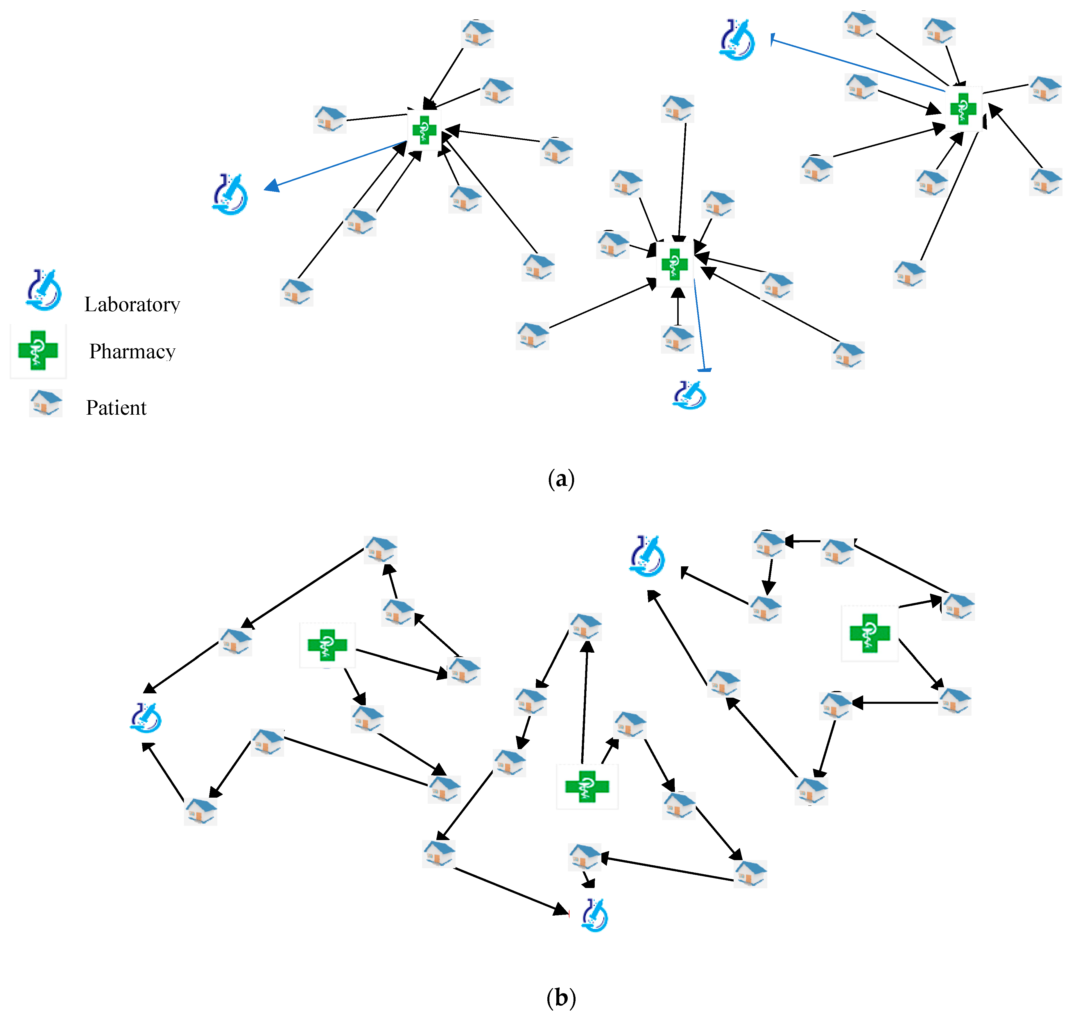
The proposed HHC model was based on the assignment, scheduling and routing decisions to obtain a valid plan for caregivers to fulfill the demand of patients. In this regard, caregivers start from their associated pharmacy. Next, they visit all of the patients and go back to the laboratory to analyze the biological samples and the treatments taken from the patients. Generally,
Figure 1 shows a graphical illustration of the proposed problem. First of all, the patients should be assigned to the closest pharmacy to ease the serving patients. Accordingly, each pharmacy should be allocated to its nearest laboratory. In this example (
Figure 1a), 24 patients were assigned to three pharmacies and laboratories accordingly. This step clusters the patients to reduce the total cost of each pharmacy. Then, the scheduling and routing decisions are made. The proposed approach determines the availability of patients and caregivers as well as their required services, in each period. Accordingly, a solution for the first period (
t) (
Figure 1b) and the second one (
t+1) (
Figure 1c) are illustrated to better observe the difference between the solutions for two consecutive periods. In the following, we first describe the proposed HHC system in details. Next, the main assumptions are provided. Finally, the deterministic model and its robust version are established.
3.1. Problem Description
The proposed HHC system is in line with recent studies in this research area [
1,
4,
5,
10,
11,
13,
14]. Assume that there is a city or town with
V patients and there are
P pharmacies and
L laboratories. A company wants to support home care services. Each pharmacy has
caregivers which are composed of four categories including a set of doctors, nurses, physiotherapists and nutritionists to provide a full range of home care services. The working time of each service is different regarding the history and type of patients’ disease (
). Each day has two period and each period is 8 h. In each period, patients may need a specific type of services (
). Each caregiver should start from his/her pharmacy. After visiting the patients, he/she comes back to his/her laboratory. This company should provide a fixed fee for hiring the caregivers in each period (
). Regarding the type of service required by patients, they should pay a cost for this service (
). If a caregiver works more than the allowable maximum time in each period, the overtime fee for the caregiver (
) is applied. Each caregiver utilizes one vehicle and accordingly, there is a transportation cost (
). Moreover, the distances among patients (
), pharmacies and patients (
) and pharmacies and laboratories (
) are based on Euclidean distance. There is also an anticipated traveling time from two patients (
). In addition, an allocation cost is associated with the distance (
). In the proposed problem, there is a time window limitation for patients regarding the earliest (
) and the latest time (
) of availability. In addition, the caregivers may not be available for all of the periods (
). The caregiver may need a rest for some periods. Based on these suppositions, the proposed HHC problem not only aimed to optimize the total cost but also the total unemployment time of caregivers and care continuity.
3.2. Assumptions
The proposed HHC problem was established under the following assumptions:
The proposed HHC has three objective functions and it is classified as multi-period, multi-depot and multi-service.
A multi-objective, mixed-integer non-linear programming approach is utilized to formulate the proposed problem.
For the robust version of the model, a scenario-based method is then generated with regards to uncertain parameters.
The travel and service times as well as the patients’ availability are the main uncertain factors.
The caregivers are composed of doctors, nurses, physiotherapists and nutritionists who can provide a full range of home care services. In the proposed model, it is assumed that a caregiver can serve as a nurse and or nutritionist for example.
The locations of pharmacies and laboratories are predefined. The number of pharmacies and laboratories are the same.
The demand of patients are home care services and they must be fulfilled. The shortage is not allowed in the model.
In each period, the caregivers’ start point is from their associated pharmacy and they go back to their associated laboratory after visiting the patients.
The working time regarding each type of service and traveling time between two patients are uncertain.
The caregiver may not be available for all of the periods.
There is an uncertain time window for availability of patients in each period.
To hire the caregivers, there are a fixed cost, service cost and the cost of overtime working, which are considered in the total cost.
Balancing the working time is considered by the unemployment time and overtime constraints, simultaneously.
The model avoids the unemployment time of caregivers in the second objective function.
Care continuity is handled by minimizing the number of patients allocated to the caregivers. It can avoid fatigue of caregivers and increase the quality of care.
3.3. Deterministic Model
To define the main deterministic model, the main notations including indices, parameters and decision variables are introduced as follows:
| Indices: |
| Patients, |
| Pharmacies, |
| Laboratories, |
| Caregivers, |
| Home care services related to the expertise of caregivers,
|
| Time periods, |
| Parameters: |
| Distance of two patients i and j |
| Distance of pharmacy p and patients i |
| Distance of laboratory l and pharmacy p |
| Distance of laboratory l and patients i |
| Transportation cost per unit of distance regarding the caregiver n working for pharmacy p |
| Allocation cost |
| Fixed cost of hiring the caregiver n for pharmacy p regarding service type k in the period t |
| Service cost for caregiver n working for pharmacy p regarding service type k in the period t |
| Overtime cost for caregiver n working for pharmacy p regarding service type k in the period t |
| Earliest availability for patient i in the period t |
| Latest availability for patient i in the period t |
| 1, if the caregiver n working for pharmacy p is available for the period t; otherwise, 0 |
| 1, if the caregiver n working for pharmacy p is able to supply the service k required from patient i; otherwise, 0 |
| 1, if the patient i needs the service k in the period t; otherwise, 0 |
| Traveling time from patient i to j |
| Anticipated time to serve patient i for service k in the period t |
| Maximum allowable time for caregivers to work in each period |
| Number of caregivers working for pharmacy p |
| A big scalar |
| Decision variables: |
| 1, if the caregiver n which starts from pharmacy p and ends with a laboratory, and does the service k visits the patient i before j in the period t; otherwise, 0 |
| 1, if the patient i allocates to pharmacy p to receive home care services; otherwise, 0 |
| 1, if the pharmacy p allocates to laboratory l; otherwise, 0 |
| 1, if the patient i with required service k is allocated to caregiver n starting from pharmacy p in the period t; otherwise, 0 |
| Starting time to visit patient i by caregiver n working for pharmacy p in the period t |
| Overtime for caregiver n working for pharmacy p regarding the service k in the period t |
| Unemployment time for caregiver n working for pharmacy p regarding the service k in the period t |
The developed multi-objective, mixed-integer non-linear programming approach to formulate the proposed HHC problem is given below:
The first objective () as given in Equation (1) aims to minimize the total cost of system. The two first terms are to compute the assignment costs. The second term is the transportation cost. The service costs as the variable cost for the caregivers as well as the fixed and overtime costs are calculated by the fourth to sixth terms in the first objective function.
The second objective () as given in Equation (2) minimizes the unemployment time for the caregivers. Lastly, the third objective function (6) optimizes the continuity of care by reducing the number of patients visited by the caregivers. This objective is a min–max function. Accordingly, the maximum number of patients for each caregiver is minimized by Equation (3).
Equation (4) is the correlation of assignment of pharmacies and laboratories to the routing and scheduling decisions. Equations (5) and (6) ensure that each pharmacy should be allocated to only one laboratory. Similarly, Equations (4) and (7) mean that a caregiver who is working in pharmacy p is able to visit the patient i, if this patient was assigned to this pharmacy. As such, each patient should be assigned to only one pharmacy as given in Equation (8). Moreover, Equation (9) shows the allocation of caregivers and patients and its correlation to the routing and scheduling decisions. Equation (10) shows that the demand of each patient should be supplied. Equation (11) ensures that each caregiver visits and leaves the patient. With regards to the VRPTW models, this limitation of the model removes the infeasible sub-tours for the HHC model. Equation (12) confirms that each tour should start from a pharmacy. As such, Equation (13) reveals that the end point of each tour is the laboratory for the caregiver after visiting the patients. Equation (14) states that the availability of caregivers changes the routing and scheduling decisions. Equations (15) and (16) guarantee that the time window limitation and the relation of routing and scheduling decision to the starting time of caregivers to visit the patients. Equations (17) and (18) compute the overtime and unemployment time, respectively. Finally, Equations (19) and (20) ensure the feasibility of binary and non-negative continuous variables.
3.4. Robust Optimization Model
The proposed HHC model ignores the uncertainty for travel and service times as well as the patients’ availability (i.e.,
,
,
and
). To deal with the uncertainty, a scenario-based robust model, which is an extension to the robust optimization introduced by Mulvey et al. [
47], is developed. The main reason to select this type of uncertainty modelling approach is that this approach is able to better simulate the uncertainty with optimistic, pessimistic and realistic scenarios [
28]. Hence, this approach creates a better view to handle the uncertainty for real-world cases [
48]. Most notably, other relevant studies [
11,
42] did not use a scenario-based robust optimization approach to formulate the HHC.
Let us assume the minimization objective function given by
, where
is the objective function for each scenario,
denotes the coefficients of binary variables,
is the binary variable,
indicates the coefficients of continuous variables for each scenario and
is the continuous variable for each scenario. In this regard, the robust version of this objective is given by:
where
is the weight factor indicating the importance of each part in the objective function,
is the set of scenarios and
is the occurrence probability of each scenario. The first part of this objective function seeks to reduce the expected cost of occurrence for different scenarios according to their associated probability. The second part of this objective function seeks to reduce the variance of the objective function values for different scenarios. Following this example, the constraints are:
where
is the technical coefficient of binary variables,
denotes the technical coefficient of continuous variables and
is the right number. Typically, scenario-based models employ the binary variables in the first stage and the continuous variables for the second stage. This naming is because the binary variables are related to real-time decisions, but the second-stage variables can wait until better information is obtained about the uncertain parameters.
One of the most important drawbacks of the model presented by Mulvey et al. [
47] is the nonlinear objective function which can be linearized by two auxiliary variables and by applying linearization methods. Leung et al. [
49] proposed another variation of the robust model by adding only one auxiliary variable and less complexity in comparison with Mulvey et al. [
47]. The objective function of this model proposed by Leung et al. [
49] is:
where
is an auxiliary variable. The constraints of this model are:
Equations (24) and (25) ensure that the second part of the proposed objective function has statistical properties such as standard deviation.
Based on these definitions, we need to redefine the uncertain parameters (i.e.,
,
,
and
). With regards to the uncertainty of these parameters, three decision variables (i.e.,
,
and
) are reconsidered by the probabilistic scenarios. In this regard, only the first and second objectives are uncertain (i.e.,
and
). Here, we firstly define some new notations for the robust model which should be replaced by the aforementioned notations. The rest of the notations are exactly the same as the ones given in
Section 3.3.
| Indic: |
| Index of probabilistic scenarios, |
| Parameters: |
| Earliest availability for patient i in the period t based on the scenario s |
| Latest availability for patient i in the period t based on the scenario s |
| Traveling time from patient i to j based on the scenario s |
| Anticipated time to serve patient i for service k in the period t based on the scenario s |
| Coefficient of the second-stage variables |
| The occurrence probability of the scenario s |
| Decision variables: |
| Starting time to visit patient i by caregiver n working for pharmacy p in the period t based on the scenario s |
| Overtime for caregiver n working for pharmacy p regarding the service k in the period t based on the scenario s |
| Unemployment time for caregiver n working for pharmacy p regarding the service k in the period t based on the scenario s |
| The total cost of the HHC services based on the scenario s as the first objective |
| The total unemployment time for the caregivers based on the scenario s as the second objective |
| Additional variable to achieve the optimality robustness in the first objective based on the scenario s |
| Additional variable to achieve the optimality robustness in the second objective based on the scenario s |
Based on the robust optimization definition extended by Leung et al. [
49], the proposed multi-objective robust optimization of the proposed HHC system is modeled by the following equations:
Equations (4)–(14) and (19)
4. Heuristics
There are many studies focusing on new heuristics to address HHC models [
4,
14,
23,
45]. The main advantage of these algorithms is to have an actable computational time in comparison with metaheuristics; but they can guarantee near global optima [
12]. Due to the novelty of the proposed model, there is no available heuristic suitable for the proposed problem. Accordingly, we extent three heuristics proposed by Fathollahi-Fard et al. [
4] to meet the constraints of the proposed model. As described in
Figure 1, the first decisions, which are the same for all periods, are the allocations of pharmacies to laboratories (
) as well as the patients to the pharmacies (
). For all three algorithms, the assignment of each pharmacy is made by the following matrix:
where
is the allocation cost for pharmacies and laboratories. To assign the patients to pharmacies, we have considered not only the distance of patients to pharmacies (
) but also the distance of patients to laboratories (
). Regarding the previous allocation, the cluster of each pharmacy is based on the average distance of this parameter for each patient. Therefore, the minimum array of the following matrix for each pharmacy is the best choice to calculate the right allocation of the patients to pharmacies:
where
is the matrix to ease the allocation of patients to specify the cluster of pharmacies. In the next step, the routing and scheduling decisions of heuristics are started. To compute this variable (
), the following matrix is generated regarding a caregiver working in his/her pharmacy and patients:
where
is the traveling cost between two patients visited by the same caregiver in sequence. The main difference of heuristics is situated in this step. Their search strategy can be summarized as follows:
Heuristic 1 (H1): To compute the tour of each caregiver, among the available patients who need a specific service, the first patient of this tour is selected as the nearest one to the pharmacy as given by . The other patients are selected as the nearest ones by the associated traveling cost matrix in Equation (40) in sequence.
Heuristic 2 (H2): To compute the tour of each caregiver, among all of the available patients who need a specific service, the first one in the tour is selected as the average of the matrix given in Equation (40) in each row to find a closest patient to the others. The other patients are selected as the nearest ones in sequence.
Heuristic 3 (H3): To compute the tour of each caregiver, among the available patients who need a specific service, the first patient of this tour is selected as the furthest patient to the laboratory based on the matrix of . The other patients are selected as the nearest patient to this patient in sequence based on the matrix of traveling cost as given in Equation (40).
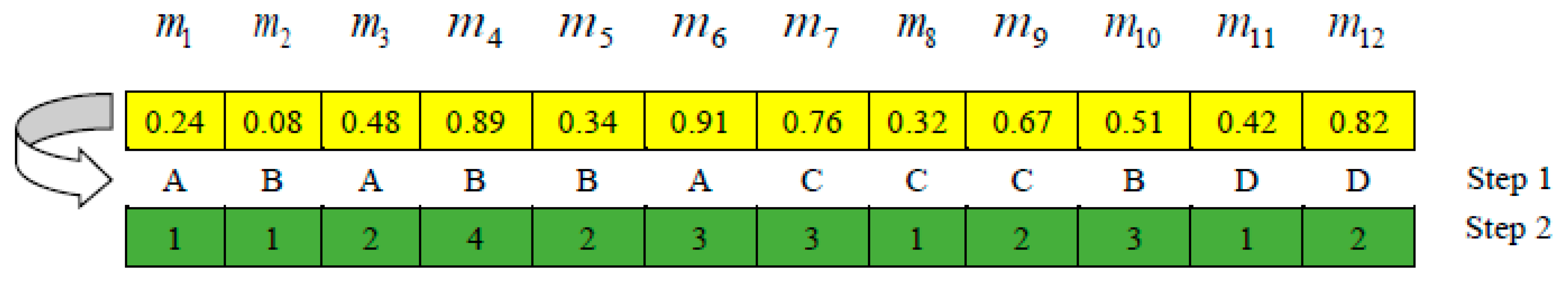
To better understand the search strategy of heuristics graphically,
Figure 2 reveals an example of five patients who need a specific service by the same caregiver. As can be seen, regarding the first heuristic (H1), the tour of this caregiver is
in which it starts with patient 3 as the closest patient to pharmacy (
Figure 2a). The tour generated by the second heuristic (H2) is
, in which it starts with patient 2 as the average of traveling cost which is the closest to other patients (
Figure 2b). The last tour generated by H3 is
and starts with patient 1 who is the furthest patient to the laboratory.
As mentioned before, the scheduling and routing decisions are the main differences of the proposed heuristics. The rest of the steps are the same and designed in a way to meet the constraints of the model to generate a feasible solution. The main challenge is the availability of patients and caregivers. To justify and clarify the calculation of scheduling and routing decisions, a numerical instance is provided by
Figure 3. This example is based on one period for a pharmacy and laboratory with 10 patients. The home care services required by patients are related to nurses and physiotherapist. The transportation cost for both caregivers are the same and are equal to two units. Based on these assumptions, we run the algorithms to find the solutions.
To implement the first heuristic (H1), first of all, for both tours, the closest patient to pharmacy would be selected. For the route of nurse, it starts with patient 3. As such, for physiotherapist, the route starts with patient 5. The nurse visits patient 7 as the closest patient to patient 3. This cycle is completed by this route . Similarly, the tour of the physiotherapist generated by H1 is . The second heuristic (H2) focuses on the average of traveling cost for each patient. In this regard, the nurse starts with patient 8 for visiting. As such, the physiotherapist visits the patient 10, first of all. The rest of visits is based on minimizing the traveling distance. Therefore, the tours of nurse and physiotherapist are, respectively, and . In the third heuristic (H3), the first patient is selected regarding the furthest one to the laboratory. In this regard, in this example, the solution for the nurse is exactly similar to the solution obtained by H1. However, the furthest patient to the laboratory for the physiotherapist is patient 2 and, in this regard, this tour is completed as . Generally, as identified from aforementioned procedures, these heuristics can provide different solutions which can give some good alternatives to the decision-maker to find a robust answer.
6. Computational Results
In this section, we firstly define the instances by different complexities. Next, all of the applied metaheuristics are tuned to have a fair comparison. To find the best efficient algorithm, the heuristic and metaheuristic algorithms are compared with regards to different criteria. To evaluate the performance of the robust optimization model, some sensitivities are performed on the key parameters. Managerial insights and main findings are finally reported from the results.
6.1. Instances
To validate the model, some benchmark tests are taken from recent studies [
4,
5,
13,
14,
41]. Based on small, medium and large-scale complexities, 12 test problems are generated as given in
Table 2. As such, the details about deterministic parameters are provided in
Table 3. With regards to the scenario-based parameters, the range of parameters based on optimistic, realistic and pessimistic scenarios is given in
Table 4. Note that the coefficient of the robust optimality (
) is 0.5 in this study. In addition, each period in the tests is 8 h and caregiver work each day in two periods at least, i.e., morning and evening. Based on the number of periods in the tests, the planning horizon may increase from 1 day to 21 days.
6.2. Parameter Tuning
Due to input parameters for metaheuristics, i.e., NSGA-II, MOMA, MOPSO, MORDA and IMORDA, here we tune these algorithms [
55,
56]. To have an unbiased comparison, the parameter tuning is very important [
30,
57]. Hence, the Response Surface Method (RSM) is one the best methods for tuning [
58]. With regards to the assessment of multi-objective optimization, the Spread of Non-dominance Solutions (SNS) [
14], Number of Pareto Solutions (NPS) [
5], Quality Metric (QM) [
41] and Hyper Volume (HV) [
57] are employed.
Generally, in the RSM method, we consider each input parameter of the algorithm as a factor with a lower and upper bound as the feasible range. Then, a linear regression model is considered to evaluate the response function as the output from one of the aforementioned Pareto metrics. The final results with regards to Pareto metrics are given in
Table 5. Using the assumed regression model, the
R-squared (
R2) for each metric and desirability (
D) show the efficiency of each metaheuristic.
6.3. Comparison of Algorithms
In this section, first of all, three proposed heuristics are employed to solve the instances. The number of objective functions and the process time are noted as given in
Table 6. Next, metaheuristics are taken into consideration by using improved solutions from heuristics. The computational time (CPU) of heuristics is presented in
Figure 7. To check the validation of their results, an epsilon constraint method is used. Their results for small sizes are reported in
Table 7 and
Table 8. Graphical presentation of these non-dominated solutions of algorithms is depicted by
Figure 8. Consequently, the results of assessment metrics of multi-objective optimization algorithms are reported in
Table 8. The behaviors of process time for these algorithms are revealed by
Figure 9. Finally, some statistical analyses are performed as given in
Figure 10 to evaluate the performance of the given algorithms.
The results of heuristics are reported in
Table 6. In each test problem, each heuristic gives a different answer except in some test problems, i.e., SP1, SP3, MP5 and MP7, in which H1 and H2 provide the same solution. To have a comparison among the heuristics, for each objective, the best value is shown in bold. In some test problems, i.e., MP5, MP8 and LP11, the solution of H2 can dominate the other algorithms’ solutions. Conversely, H1 can dominate H2 in two case studies, i.e., MP7 and LP9. Accordingly, for the first objective function (
), in the majority of cases (eight test problems), H2 shows the best optimal value. In regards to the second objective function (
), H1 and H2 are the best in five instances. Based on the third objective function (
), H2 is strongly better regarding its successful outputs in nine cases. Therefore, it seems that H2 is generally stronger than other heuristics.
What can be seen from
Figure 7 confirms that there is a set of similarities between the behaviors of heuristics. Generally, all of these algorithms are fast and can solve a large-scale problem in less than 10 s. In most cases, except in MP8 and LP9, H3 is the worst heuristic and, conversely, H2, except in MP7, LP11 and LP12, is the best algorithm in this item.
In conclusion, the H2 algorithm outperforms the two other heuristics in terms of solution quality and process time.
Here, the results of heuristics are used as the initial solutions of metaheuristics to have a better search. To validate their results, we used an Epsilon Constraint (EC) method developed by Haimes et al. [
59]. In this method, the Pareto optimal set is modified by the bounds of the objective function [
5,
41]. The formulation of this methodology based on the structure of proposed model is presented by:
Equations (29)–(37)
Equations (4)–(14) and (19)
Following this, this algorithm as given in Equation (49) solves SP1. The first objective function () is optimized accordingly. To reach the Positive Ideal Solution (PIS) and Negative Ideal Solution (NIS), other objectives (i.e., and ) are considered as the main objective instead of the first one when this algorithm runs. To generate a Pareto-based solution, the bounds of the EC method (i.e., and ) will be updated with regards to the average of the PIS and NIS.
To ease the assessment on the non-dominated (the best Pareto-based) solutions,
Table 6 gives the sorted solutions of the five metaheuristics and the EC method.
Figure 8 shows these solutions graphically. To check the performance of the algorithms’ validation, a modified NPS (MNPS) is defined by a comparison with results of the non-dominated solutions of the metaheuristics and Pareto-based solution of the EC [34; 48]. Therefore, this percentage
measures the validation. Clearly, a higher value for this percentage brings better reliability of metaheuristics solutions. Final results are given in
Table 8 for a number of small test studies.
The outputs of this validation, as illustrated in
Table 7, reveal that all of metaheuristic algorithms are reliable and generate high-quality non-dominated solutions. In addition,
Figure 8 confirms the efficiency of IMORDA in comparison with other metaheuristics closely. In conclusion, the high-quality of IMORDA is demonstrated in
Table 7 as it has 0.91 validation, which is significantly higher than for the results of NSGA-II (0.75), MOPSO (0.76), MOMA (0.68) and the original version of MORDA (0.87).
After the validation, the solutions of metaheuristics are compared with each other based on different criteria. The results of the algorithm in terms of NPS, SNS, QM and HV as well as the process time (CPU) are reported in
Table 9. In each metric, the best values are shown in bold. Generally, MORDA and IMORDA are better than other algorithms in majority of instances based on the aforementioned assessment metrics.
As may be identified by
Figure 9, there are some similarities between the computational times of the metaheuristics. It is observed that MORDA is the worst algorithm in this item, whereas MOPSO shows the best behavior. Another result is that the proposed IMORDA is slightly better than MORDA, which shows an improvement in this metaheuristic.
The results of assessment metrics are normalized by the use of the relative deviation index (RDI) to have a comparative study.
The details of this well-known transformation metric can be referred to in the literature. To examine the performance of algorithms, interval plots with the use of the RDI are provided in
Figure 10.
Based on the NPS metric (
Figure 10a), MOMA is the worst algorithm and, conversely, IMORDA is the best one. NSGA-II and MOPSO have the same behavior. As such, MORDA is better than other algorithms except IMORDA. In regards to the SNS metric (
Figure 10b), MOMA, MORDA and IMORDA are the best algorithms. As such, MOPSO and NSGA-II are the worst ones. NSGA-II shows a weak performance while IMORDA reveals a high performance. Regarding the QM metric (
Figure 10c), the proposed IMORDA is completely better than other algorithms. As such, MOPSO is the worst algorithm in this item. Based on the HV metric (
Figure 10d), there is a similarity for the algorithms. In conclusion, the proposed H2 is the best heuristic and IMORDA is the best metaheuristic.
6.4. Sensitivity Analysis
Here, we firstly examine the impact of the proposed robust model given in
Section 3.4 in comparison with the deterministic one as given in
Section 3.3. In this regard, a small test problem, i.e., SP2, is selected and the second heuristic is applied to conduct the analyses. For the robust model, we have considered all optimistic, realistic scenarios. However, for the deterministic model, only the realistic scenario is assumed to value the uncertain parameters. This comparison is shown in
Figure 11. With regards to these analyses, the performance of the robust model in the first and second objective is much better than the deterministic model.
In addition to the analyses related to the uncertainty, some sensitivity analyses based on the key parameters of the developed HHC model are performed. In this regard, five parameters including the transportation cost (
), the fixed cost of employment of caregivers (
), the service cost of caregivers (
), the overtime cost of caregivers (
) and the maximum time of working for each caregiver (
) are analyzed. In each analysis, five cases are considered. The results are reported in
Table 10,
Table 11,
Table 12,
Table 13 and
Table 14 and
Figure 12,
Figure 13,
Figure 14,
Figure 15 and
Figure 16.
Similar to other HHC studies, one of the main parameters is the transportation cost, which includes a large part of the total cost. The results of sensitivities on the transportation cost are reported in
Table 10. The behaviors of objective functions based on the normalized values are depicted by
Figure 12. From the results, it can be concluded that this parameter has no impact on the second and third objectives. This factor increases the cost significantly.
The sensitivities on the fixed cost of hiring the caregivers are reported in
Table 11. Similar to
Figure 12, the behaviors of objectives are depicted by
Figure 13. By increasing the amount of this parameter, there is no effect on the second and third objective functions. However, it can change the total cost. By growing the amount of the fixed costs, the model allocates the best caregiver with lowest values to the patients. Generally, this parameter can increase the total cost if there is no other choice for the allocation of patients.
Another main parameter of the proposed HHCP is the service cost of the caregivers. The results of sensitivities on the amount of this parameter are reported in
Table 12. The behavior of objectives based on the normalized values is given in
Figure 14. This parameter has no effect on the second and third objective functions. By increasing this parameter, firstly the total cost reduces and then it increases. The reason would be the optimal case of this parameter is found by an increase in its amount. Generally, an increase in the amount of this parameter increases the total cost as the first objective function.
The cost of overtime is analyzed by a set of sensitivity analyses as reported in
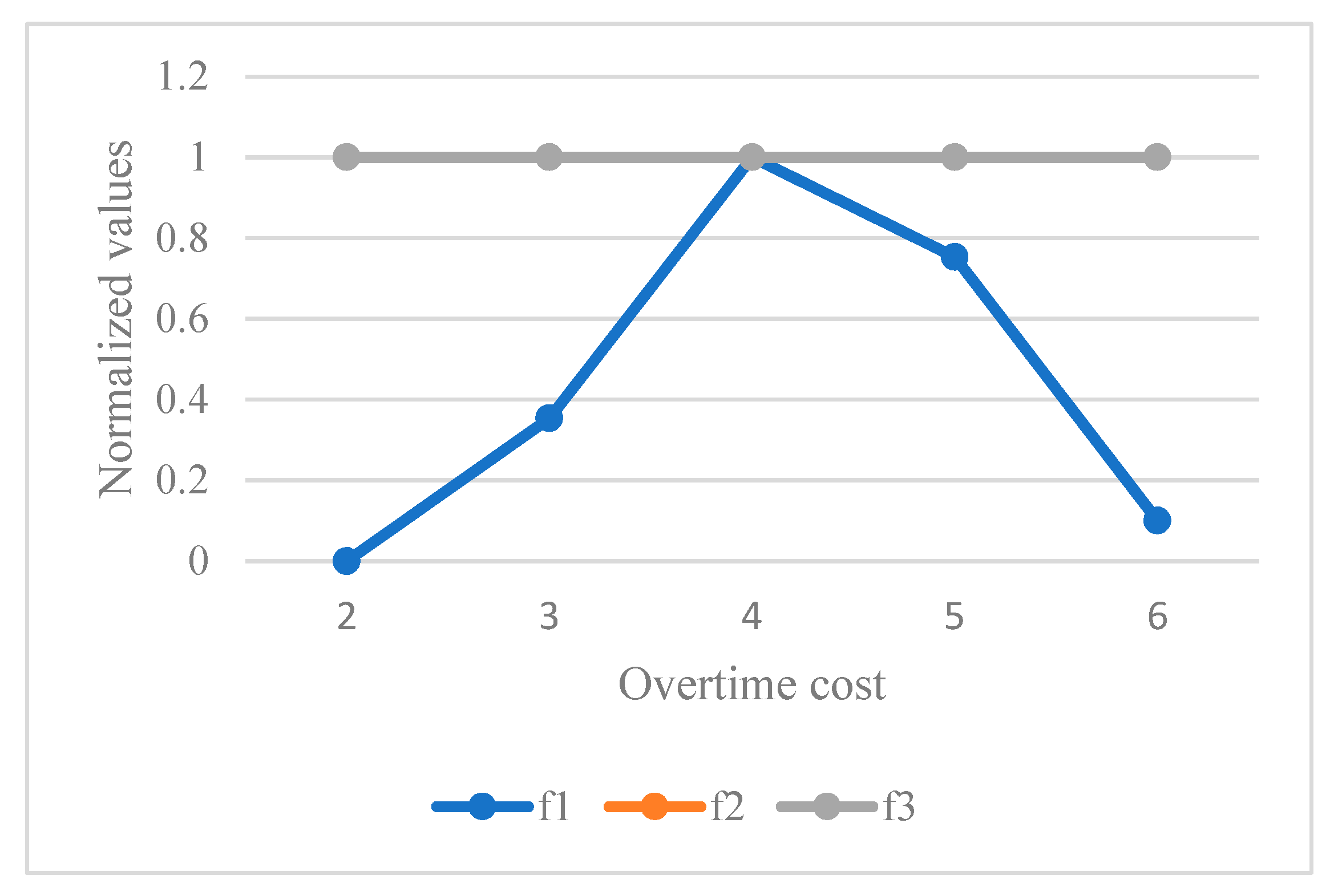
Table 13 and the behavior of algorithms is given in
Figure 15. Based on the results, this parameter has no impact on the second and third objective functions. By increasing this parameter as a penalty for the caregivers’ working, first of all, the total cost is increased. After that, it can reduce the total cost. This parameter can avoid the extra working of caregivers.
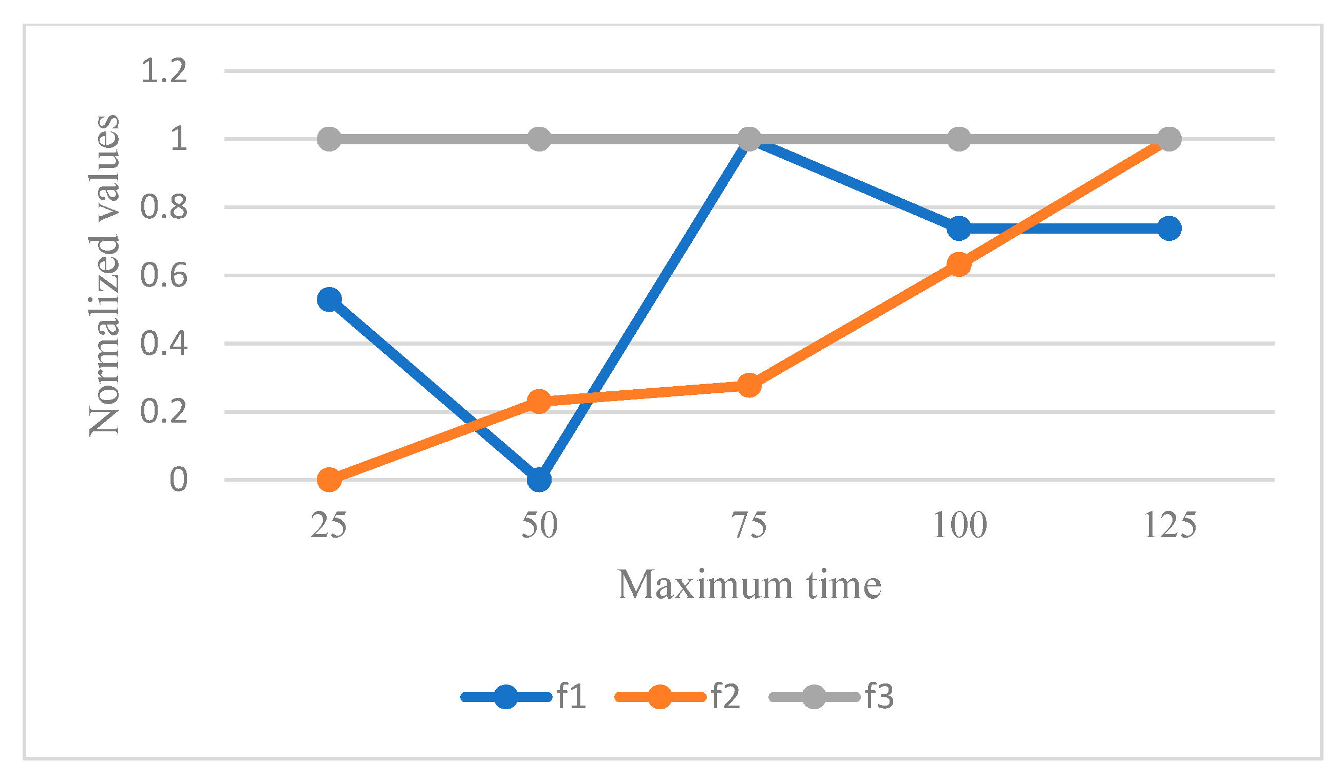
At the end, the maximum time of working for the caregivers is analyzed by some sensitivity analyses as reported in
Table 14 and
Figure 16 shows the behavior of objective functions. This parameter has no effect on the third objective function as the continuity of care. However, this parameter can increase the amount of unemployment time of caregivers by increasing the amount of maximum time in each period. Regarding the first objective function, the behavior of the total cost has firstly decreased and then increased. Hence, this parameter has an impact on the amount of optimal solution and the best case of allocation and routing decisions.
6.5. Discussion of Results
Conventionally, operational HHC planning aims to simulate the routing and scheduling of caregivers to visit the patients independently, using a simplified model. From a majority of studies, especially in developed and western countries, the care of aging population is a grand challenge. However, a simple HHC model fails to address satisfactorily all of the real concepts in the HHC companies including different HHC services, balancing the working time of the caregivers and care continuity as well as different difficulties to provide a plan for caregivers’ activities such as uncertainty of travel and service times along with unpredicted unavailability of the patients. This study developed a new, efficient and practical model as a multi-objective robust optimization of the HHC services as an extension to vehicle-routing optimization. Applicability needs a multi-objective robust optimization to control uncertainty and to accommodate unemployment time and continuity of care operated across an HHC network design. Efficiency needs a robust and fast solution algorithm to solve this complex combinatorial optimization problem adequately.
The viability of an HHC optimization with three conflicting objectives and real-life constraints is highly demonstrated by the results of this study. A multi-objective robust optimization is formulated by a scenario-based mixed-integer non-linear programming model. In addition, a new adaptive extension of MORDA (IMORDA) is also introduced. This study proposes three fast heuristics to find an optimal solution in an acceptable computational time to support the initial solutions of metaheuristics, i.e., MOPSO, NSGA-II, MOMA, MORDA and IMORDA as the best efficient method.
Obviously, the proposed HHC is more complex than the majority of HHC studies. This study not only contributes to the total cost as the first objective but also it considers the social impacts of an HHC system to satisfy the caregivers by working-time balancing and to improve the quality of the care by optimizing care continuity. A full range of cares by using doctors, nurses, physiotherapists and nutritionists is supported as well. The unemployment time of caregivers as the second objective can help the system to work substantially. As such, the third objective function to optimize the continuity of care can increase the quality of care by reducing the total number of patients visited by the caregivers. The applicability of the developed heuristic and the proposed metaheuristic, so-called IMORDA in this study, provides great encouragement for developing new metaheuristics.
Although a majority of HHC studies are mainly focusing on metaheuristic solutions, the use and development of heuristics is still scarce in the literature. Three heuristics in this study are fast and achieved the optimal solutions of the proposed HHC problem. Among all heuristics, the application and testing of the second heuristic to a more representative HHC model creates new practical highlights. More justifications and analyses to our heuristics are warranted.
This study conceptually shifts HHC management to the multi-objective robust optimization of HHC management to provide a robust plan of the logistics activities of the caregivers with the working-time balancing and care-continuity suppositions. This study introduces multi-service HHC services including different skills of the caregivers: doctors, nurses, physiotherapists and nutritionists. This variety can support a full range of home care operations as per the needs of patients.
Based on aforementioned findings, some managerial highlights can be concluded from the results, as the proposed multi-objective robust optimization of the HHC services is very complex. This fact strongly encourages more development and application of high-performance algorithms such as IMORDA as given in
Figure 10 and our second heuristic (H2) as illustrated in
Table 6. Another practical insight refers to the analyses of the robust model in comparison with the deterministic model as given in
Figure 11. The dynamic sensitivity of the objective functions, illustrated in
Figure 12,
Figure 13,
Figure 14,
Figure 15 and
Figure 16, is highly visualized. Most especially, the volatility of the total deviation from the unemployment time of caregivers (
f2) to variations in the cost of transportation, shown in
Figure 12, warrants further investigation on this issue. Similarly, the amount of maximum time of working in each period can affect both the total cost and unemployment time. Conversely, the continuity of care responses had no impact on variations in all the analyses. This indicates the need for more detailed investigation.
In conclusion, our results are useful for both healthcare and academic practitioners to examine the planning of HHC services under uncertainty. Certainly, some other parameters with regards to other real concepts of HHC organizations are still needed in practice.
7. Conclusions and Future Remarks
In this article, the viability of an HHC optimization problem definition by three conflicting objectives and real-life constraints using a multi-objective, scenario-based, mixed-integer non-linear programming approach was demonstrated. This study applied a multi-objective robust optimization model to HHC services. An extension to the VRPTW, which is multi-depot, multi-period and multi-service, was developed to optimize the total cost, unemployment time and care continuity. This study also contributed to the working-time balancing of the caregivers by considering unemployment time and overtime constraints. As the proposed problem is NP-hard and complex, three fast heuristics to better solve the problem in an acceptable process time were designed. An improvement to the multi-objective RDA (IMORDA) was shown to do especially well given the definition of the proposed HHC problem. In addition, all methods were tuned and compared across four popular assessment metrics including HV, QM, SNS and NPS. Finally, the performance and efficiency of the second heuristic (H2) and our new metaheuristic (IMORDA) are concluded from the results.
Although the proposed HHC is clearly more complex than a majority of HHC papers, there are still some new additions for future studies. Considering the green emissions of routing, optimization faces a new challenge with HHC management to consider triple lines of sustainability simultaneously. Adding travel balancing in addition to working-time balancing makes the model more complex and interesting. Contributing to machine-learning algorithms is very useful for providing a simulation model for HHC activities. Last but not least, application and development of our heuristics and metaheuristics for other optimization problems in logistics network design is another good continuation for further research.


