Abstract
One of the main problems faced in coastal management is the loss or destruction of beaches due to erosion. A considerable diversity of factors is involved in coastal erosion, which makes it a complex system to study. The quality of the material that constitutes the beach, as well as the choice of appropriate materials for its nourishment are two of the main ones. Therefore, to make future nourishment projects more sustainable and durable, this work proposes a sediment quality classification based on the physical properties and wear process obtained through laboratory tests. The study of these variables, using principal component analysis, discriminant analysis and ANOVA, has divided the quality of 70 samples into three main groups. A Sediment Quality Classification Index (SQCI) is proposed, which categorizes the quality of the material into poor, regular or good, providing the coastal engineer with a simple tool to ensure more sustainable beach nourishments.
1. Introduction
The erosion of sandy beaches and the scarcity of natural material for artificial beach nourishment is a serious problem worldwide [1]. The sedimentary budget and the capacity to maintain coastal morphology is based on the balance between the generation, destruction and transport of sediments [2]. Determining the influence of the diverse factors involved in sediment erosion is important to minimize coastal erosion [3]. Erosion begins with the transport of sediment particles by waves and currents (near-shore rip or long-shore) [4,5,6]. Transport can result in the loss of beach sediment over short to medium time frames due to passing the depth of closure (in reference to the active zone of sediment transport according to Hallermeier [7]) where particles will not be returned to the beach even in storm events [7], or to the wear and consequent loss of size of the particles, by breakage, rounding or dissolution [8]. The results of various studies show that the different components that form the sediment exert significant control over its durability [9,10].
The concept of sediment durability can be associated with material fatigue, i.e., material breakage produced by long-lasting dynamic stresses [11]. Although there are many studies on the fatigue of materials such as steel and concrete, the study on sediment, and specifically on beach sand is much more limited [12]. Even so, the few studies conducted show that the defects of these particles, like micro cracks, pores, grain boundaries, etc. [13], are the beginning of cracking and brittle breakage of the material [14].
To know the behavior of the material for intervening on the coasts with the least possible impact, the accelerated particle wear test (APW) enables the study of the wear behavior suffered by the sand particles in the swash zone of the beach [8]. In addition, the mineralogical composition and morphology of the particles play an important role in their durability [15,16], and consequently in the retreat of the shoreline.
The number of factors involved in both shoreline erosion (with continuous temporal and spatial changes) and sediment wear complicate attempts to accurately model this complex system. The projected actions on the coast must be developed sustainably with criteria of the circular economy. Thus, knowing the useful life period (durability or period prior to complete sediment weathering) of the material to be used in coastal nourishment helps to optimize resources, reducing the number and cost of nourishments and the effects on ecosystems due to the reduction in negative effects caused during the fills (water turbidity, possible partial burying of vegetation species, etc.). This implies lowering the impact of these actions on the environment, making the coastal recovery process more sustainable.
In this work, a classification of sediment quality is established based on an index generated from the physical characteristics of the sediment and the results of the APW test. Principal component analysis, discriminant analysis and ANOVAs were conducted to establish three groups of sediment quality (good, regular and poor). This offers the coastal engineer a tool to determine the most sustainable sediment (most economical and durable material of those available) to be used in beach nourishment projects.
2. Materials and Methods
2.1. Sampling
A total of 70 sand samples were collected mainly from the coast of Spain (61 samples) (Figure 1). Six samples from other countries (2 from Thailand, 1 from Mexico, 2 from the Dominican Republic and 1 from Italy) were also included along with 3 artificial samples (silica sand standardized in two different granulometries and an artificial mixture formed by sand from a quarry and sand from Guardamar beach, Spain). For more information on the samples see Supplementary File S1. The use of artificial samples is because they were going to be used in the nourishment of a beach in the province of Alicante, although finally, it was not executed, but the APW test was performed. These samples have a slightly larger size than the Alicante beaches, so APW tests were applied to the mixture between the artificial sample and the sand from the Guardamar beach to check the nourishment behavior. The natural samples were collected from the swash zone of the beach and were not analyzed for mineralogical composition. At least 75 g were collected for each of the samples to enable the accelerated particle wear test to be performed.
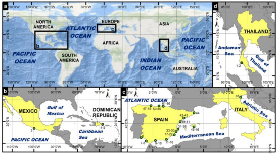
Figure 1.
(a) Location of sediment samples collected from beaches in (b) Mexico and Dominican Republic, (c) Spain and Italy and (d) Thailand.
The samples collected have a median sediment size between 0.143 and 1.059 mm, and an overall average median value of 0.313 mm.
2.2. Accelerated Particle Wear Test (APW)
The APW test proposed by Lopez et.al. [8] was used to determine the wear of the collected sand samples. The test consists of stirring with a magnetic stirrer 75 g of sediment and 500 mL of seawater. Cycles of 24 h are applied until 50% of the sample is reduced to sizes smaller than 0.063 mm. After each cycle, the texture of the sample is analyzed to determine its median size. The granulometries were made following the UNE-EN ISO 17892-4:2019.
2.3. Modelling
To achieve the sediment quality classification, 4 variables were used for each of the samples used: (i) the median size of the initial sample sediment in millimeters (D50), (ii) the total number of cycles in the APW (Cycles), (iii) the percentage of weight lost during the first cycle in the APW expressed as a fraction of unity (W1) and (iv) the relationship between the accumulated weight lost between the first and the penultimate cycle and the number of cycles elapsed (mn). When the number of total cycles was less than or equal to 2, the values of the penultimate cycle were replaced by the values of the last cycle. Both W1 and mn values are negative. Table 1 shows the descriptive values of each of the four variables.

Table 1.
Descriptive statistics of the used variables. Values refer to overall samples (n = 70).
Firstly, a principal component analysis (PCA) was conducted. This procedure reduces the dimension of the data matrix (70 samples × 4 variables) providing new non-dimensional variables. In the case study, since the number of variables is small, the intention was to use the properties of the resulting factors for the construction of an index.
Once the factors were obtained, an index (Sediment Quality Classification Index, SQCI) was constructed and transformed into a range between 0 and 1 using Equation (1). Observing the obtained values, three classification levels were determined: 1—poor, 2—regular, and 3—good. The validity of these ranges was validated by performing a discriminant analysis in which the four original variables (D50, Cycles, W1, and mn) were introduced as independent variables and the quality classification level (1—poor, 2—regular, and 3—good) as a grouping variable. The proposed classification was compared with the classification obtained in the discriminant analysis to determine whether the proposed ranges for the index were valid or not. This process was repeated several times until the proposed ranking coincided 95% with the ranking of the discriminant analysis. In Section 3 below, only the final result is shown.
To determine if there were differences between the variables in each of the three proposed classification groups, an ANOVA was performed.
Finally, and to validate the proposed index, 28 new samples of different materials from quarries (Table 2) were classified using both the classification index and the discriminant analysis. In this way, the suitability of the quarry material for use in possible coastal nourishment can be determined.
Table 2.
Descriptive statistics of the variables of the samples used in the validation. Values refer to overall samples (n = 28).
3. Sediment Quality Classification Index (SQCI)
The PCA showed only one component in its result, i.e., that the four variables originally introduced became one. The coefficients needed for the calculation of the main component scores are shown in Table 3.
Table 3.
Coefficient matrix for the calculation of component scores.
Converting to values of 0 and 1, the value obtained using the PCA (named Sediment Quality Classification Index) in each one of the study samples is shown in Figure 2. A priori, it can be seen that the samples with a longer duration in the APW test present a higher value of the index. From the observation of the values, the following three classification ranges are established:
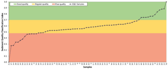
Figure 2.
Index established based on the principal component analysis (PCA) values and proposed classification levels (poor, regular and good) for 70 samples. Samples 68, 69 and 70 are the artificial ones.
- Poor quality—SQCI < 0.48;
- Regular quality—SQCI between 0.48 and 0.70;
- Good quality—SQCI > 0.70.
This proposed classification was used to perform the discriminant analysis, which provided two canonical functions (Table 4). The eigenvalues of the two functions that constitute the model are very unequal. The first function explains 79.2% of the variability available in the data, while the second function only explains 20.8%. Similarly, the canonical correlation of the first function is very strong (0.879), while that of the second function is strong (0.686) according to the scale of Evans [17].
Table 4.
Eigenvalues obtained from the discriminant analysis.
Wilks’ Lambda contrasts hierarchically the significance of the two obtained functions (Table 5), that is, it contrasts the hypothesis of equality of the centroids. As can be observed, the value of Wilks’ Lambda statistic decreases with each step of the model, which indicates that, as variables are incorporated into the model, the groups are less and less overlapping. The first line (1 through 2) contrasts the null hypothesis that the complete model (both discriminant functions taken together) does not enable the means of the groups to be distinguished. Since the value of Wilks’ Lambda has a critical level (Sig. = 0.000) lower than 0.05, it is possible to conclude that the model can distinguish significantly between the groups. In the second line (2) it is contrasted if the means of the groups are equal in the second discriminant function. Wilks’ Lambda takes a value very close to 1, but the critical level (Sig. = 0.000) is less than 0.05, so it can be concluded that the second function discriminates between at least two of the groups.
Table 5.
Wilks’ Lambda.
The matrix of standardized coefficients (Table 6) contains two discriminant functions, the first one being the one with the highest discriminative capacity. This first function discriminates, fundamentally, by the number of cycles. The second function attributes the highest weighting to mn.
Table 6.
Standardized coefficients of the canonical discriminant functions.
Table 7 shows the location of the centroids in each of the discriminant functions. Both functions distinguish with great precision between the different sediment qualities since only 3% of the samples studied do not match the defined classification (Figure 3). The first canonical function allows effective differentiation between the poor- and good-quality sediment since both centroids are strongly separated from each other (negative and positive zone of the axis, respectively). Additionally, it allows the regular quality to be distinguished, although if only one canonical function was used there could be confusion between it and the poor and good qualities since the regular quality centroid is close to the other two. The second canonical function mainly distinguishes the regular quality from the other two classifications, since the centroid of the regular quality is in the positive zone of the axis, while the centroids of the other two qualities are in the negative zone.
Table 7.
Canonical functions at the centroids of the groups.
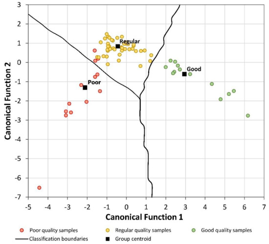
Figure 3.
Territorial map and values of the canonical functions for each of the studied samples.
Figure 3 shows the territorial map (space corresponding to each of the groups in the plane defined by the two discriminant functions: the first function on the abscissa axis and the second function on the ordinate axis). The centroids of each group are represented by squares. Observing the location of the centroids in the figure, it can be seen that the first function has greater discriminant capacity than the second since the centroids are dispersed or moved further away in the horizontal direction compared to the vertical. Since the discriminant provides the same values as those proposed for the classification of the sediment, except for 22 (Los Locos beach, Torrevieja), 43 (Levante beach, Salou) and 9 (Cristo beach, Estepona), which are within the limits of the territorial map, it can be concluded that the established ranges are valid for classifying the quality of the sediment.
Through the ANOVA, the differences between the four variables are studied according to quality classification of the sediment. The main difference between groups is shown in the number of cycles in the APW test (Figure 4b). The poor-quality sediment has an average of 2.5 cycles, while the regular-quality sediment has an average of 6.16, and the good-quality sediment has an average of 18.8 cycles. The rest of the variables present differences between two groups; the median size shows significant differences between good, poor and regular quality (Figure 4a). The weight loss in the first cycle (W1), and the relationship between the accumulated weight lost between the first and next-to-last cycles and the number of cycles elapsed (mn) also show differences between sediment quality classes (Figure 4c,d, respectively).
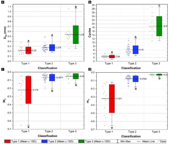
Figure 4.
Classification of sediment samples (n = 70). (a) Median sediment size as a function of sediment type; (b) number of cycles in the accelerated particle wear test (APW) test as a function of sediment type; (c) W1 as a function of sediment type; (d) mn as a function of sediment type. * The letters a, b, c represent the equality or difference between groups according to the ANOVA.
Finally, using both the index (SQCI) obtained from the PCA and the discriminant functions, 28 new samples from quarry material are classified. Figure 5 and Figure 6 show that the results of both analyses are in complete agreement. Analyzing the results in detail, 68% of the samples are classified as poor quality, which is mainly due to the number of cycles in the APW test; according to the canonical function 1 of the discriminant analysis (Table 6) the Cycles are the variable that most influences the classification with a value of 0.69. To discover, in more depth, why these quarry samples present such poor quality, it will be necessary to undertake detailed analysis of the mineralogical composition and morphology of the particles, as suggested by different authors [14,18]; if only the median size of these samples is considered (0.304 mm) their classification should be between regular and good, and not poor as obtained (Figure 5 and Figure 6).
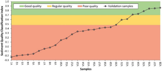
Figure 5.
Values of the sediment quality classification index (SQCI) in the validation samples.
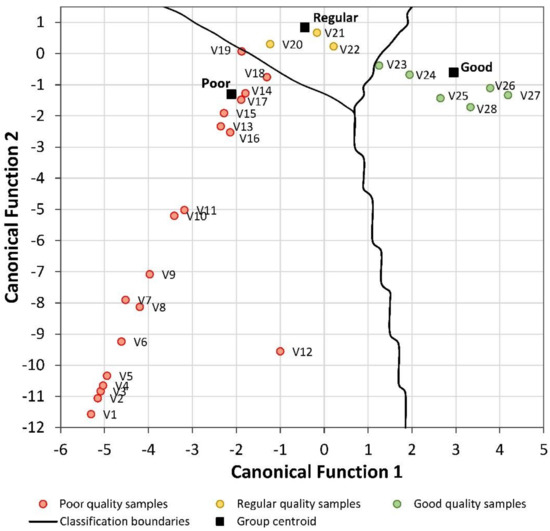
Figure 6.
Territorial map and canonical function values for the validation samples.
Therefore, the final equation of the Sediment Quality Classification Index to employ the four variables (without standardizing) will be Equation (2), using the ranges of poor quality SQCI < 0.48, regular quality 0.48 < SQCI < 0.70, and good quality SQCI > 0.70.
4. Conclusions
Analyzing the behavior of sediments to minimize the impact on coastal actions is extremely complex because several variables are involved. This study proposes an index (SQCI) that considers both physical and sediment wear parameters.
- After performing a principal components analysis, discriminant analysis and ANOVA, a sediment quality index (SQCI) has been established, which distinguishes the quality of the sediment according to its physical characteristics (median sediment size, D50) and its behavior against the accelerated wear test of particles involving number of cycles (Cycles), weight loss in the first cycle (W1), and the relationship between the weight lost between the first and the penultimate cycle and the number of cycles (mn).
- Three qualities have been established: (1) poor with SQCI values lower than 0.48; (2) regular with SQCI values between 0.48 and 0.7; (3) good with SQCI values higher than 0.70.
With this index, the coastal engineer will be able to choose sand of satisfactory quality (good) for a beach fill project, making the nourishment sustainable both economically and environmentally.
Supplementary Materials
The following are available online at https://www.mdpi.com/2071-1050/13/5/2633/s1, Supplementary File S1.
Author Contributions
Conceptualization, L.A. and Y.V.; methodology, I.L. and Y.V.; software, J.I.P.; validation, J.I.P. and Y.V.; formal analysis, I.L. and Y.V.; investigation, J.I.P. and A.J.T.-A.; resources, A.J.T.-A. and L.A.; data curation, J.I.P. and A.J.T.-A.; writing—original draft preparation, J.I.P. and A.J.T.-A.; writing—review and editing, I.L.; visualization, Y.V.; supervision, I.L. and A.J.T.-A.; project administration, I.L.; funding acquisition, I.L. and J.I.P. All authors have read and agreed to the published version of the manuscript.
Funding
This research was funded by Generalitat Valenciana through the project GV/2019/017 (Estudio sobre el desgaste y composición de los sedimento y su influencia en la erosión de las playas de la Comunidad Valenciana).
Institutional Review Board Statement
Not applicable.
Informed Consent Statement
Not applicable.
Data Availability Statement
Data is contained within the article or supplementary material. The data presented in this study are available in Supplementary File S1.
Conflicts of Interest
The authors declare no conflict of interest. The funders had no role in the design of the study; in the collection, analyses, or interpretation of data; in the writing of the manuscript, or in the decision to publish the results.
References
- Amin, S.K.; El-Sherbiny, S.; Abo-Almaged, H.; Abadir, M. Recycling of Marble Waste in the Manufacturing of Ceramic Roof Tiles. In Waste Valorisation and Recycling; Springer: Berlin, Germany, 2019; pp. 119–127. [Google Scholar]
- Ford, M.; Kench, P.S. The durability of bioclastic sediments and implications for coral reef deposit formation. Sedimentology 2012, 59, 830–842. [Google Scholar] [CrossRef]
- Widdows, J.; Brown, S.; Brinsley, M.D.; Salkeld, P.N.; Elliott, M. Temporal changes in intertidal sediment erodability: Influence of biological and climatic factors. Cont. Shelf Res. 2000, 20, 1275–1289. [Google Scholar] [CrossRef]
- Allen, J.R. Physical Processes of Sedimentation; American Elsevier Pub. Co.: Amsterdam, The Netherlands, 1970. [Google Scholar]
- Komar, P.D. Selective grain entrainment by a current from a bed of mixed sizes: A reanalysis. J. Sediment. Res. 1987, 57, 203–211. [Google Scholar]
- van Rijn, L.C. Unified view of sediment transport by currents and waves. I: Initiation of motion, bed roughness, and bed-load transport. J. Hydraul. Eng. 2007, 133, 649–667. [Google Scholar] [CrossRef]
- Hallermeier, R.J. Seaward Limit of Significant Sand Transport by Waves: An Annual Zonation for Seasonal Profiles; DTIC Document: Washington, DC, USA, 1981. [Google Scholar]
- López, I.; López, M.; Aragonés, L.; García-Barba, J.; López, M.P.; Sánchez, I. The erosion of the beaches on the coast of Alicante: Study of the mechanisms of weathering by accelerated laboratory tests. Sci. Total Environ. 2016, 566, 191–204. [Google Scholar]
- Woodroffe, C.D.; Samosorn, B.; Hua, Q.; Hart, D.E. Incremental accretion of a sandy reef island over the past 3000 years indicated by component-specific radiocarbon dating. Geophys. Res. Lett. 2007, 34. [Google Scholar] [CrossRef]
- McLean, R.F.; Stoddart, D.R. Reef island sediments of the northern Great Barrier Reef. Philos. Trans. R. Soc. Lond. 1978, 291, 101–117. [Google Scholar]
- Attewell, P.B.; Farmer, I.W. Fatigue behaviour of rock. Int. J. Rock Mech. Min. Sci. Geomech. Abstr. 1973, 10, 1–9. [Google Scholar] [CrossRef]
- Haghgouei, H.; Baghbanan, A.; Hashemolhosseini, H. Fatigue life prediction of rocks based on a new Bi-linear damage model. Int. J. Rock Mech. Min. Sci. 2018, 106, 20–29. [Google Scholar] [CrossRef]
- Justo-Reinoso, I.; Srubar, W.V.; Caicedo-Ramirez, A.; Hernandez, M.T. Fine aggregate substitution by granular activated carbon can improve physical and mechanical properties of cement mortars. Constr. Build. Mater. 2018, 164, 750–759. [Google Scholar] [CrossRef]
- Chiva, L.; Pagán, J.I.; López, I.; Tenza-Abril, A.J.; Aragonés, L.; Sánchez, I. The effects of sediment used in beach nourishment: Study case El Portet de Moraira beach. Sci. Total Environ. 2018, 628–629, 64–73. [Google Scholar] [CrossRef] [PubMed]
- Zarasvandi, A.; Moore, F.; Nazarpour, A. Mineralogy, Mineralogy and morphology of dust storms particles in khuzestan province: XRD and SEM analysis concerning; Tarkib-e kani shenakhti va rikht shenasi-e zarat-e tashkil dahande-ye padide-ye gard va ghobar dar ostan-e khuzestan ba tekie bar analiz-haye XRD va tasavir-e SEM. Iran. J. Crystallogr. 2011, 19, 511–518. [Google Scholar]
- Roberts, J.; Jepsen, R.; Gotthard, D.; Lick, W. Effects of particle size and bulk density on erosion of quartz particles. J. Hydraul. Eng. 1998, 124, 1261–1267. [Google Scholar] [CrossRef]
- Evans, J.D. Straightforward Statistics for the Behavioral Sciences; Thomson Brooks/Cole Publishing Co.: Pacific Grove, CA, USA, 1996. [Google Scholar]
- Pagán, J.I.; López, M.; López, I.; Tenza-Abril, A.J.; Aragonés, L. Causes of the different behaviour of the shoreline on beaches with similar characteristics. Study case of the San Juan and Guardamar del Segura beaches, Spain. Sci. Total Environ. 2018, 634, 739–748. [Google Scholar] [CrossRef] [PubMed]


Publisher’s Note: MDPI stays neutral with regard to jurisdictional claims in published maps and institutional affiliations. |
© 2021 by the authors. Licensee MDPI, Basel, Switzerland. This article is an open access article distributed under the terms and conditions of the Creative Commons Attribution (CC BY) license (http://creativecommons.org/licenses/by/4.0/).