Article

Structural and Efficiency Effects of Land Transfers on Food Planting: A Comparative Perspective on North and South of China

Business School, Xiangtan University, Xiangtan 411105, China
*
Author to whom correspondence should be addressed.
Sustainability 2021, 13(6), 3327; https://doi.org/10.3390/su13063327
Submission received: 8 February 2021 / Revised: 11 March 2021 / Accepted: 14 March 2021 / Published: 17 March 2021
(This article belongs to the Section Sustainable Food)

Abstract

:
This paper uses a multi-period PSM-DID model to explore the impact of land transfers on food production from a spatial perspective and analyses the income effects, scale effects, and structural effects of such transfers. The empirical results are as follows. (1) Land transfers have reduced the proportion of food crops planted by farmers, and the planting structure has shifted towards cash crops, which has obvious structural effects. (2) The impact of land transfers on the planting structure is spatially heterogeneous. Land transfers are more common in the south than in the north. Land transfers have reduced wheat planting in the north, while rice planting has been reduced in the south. (3) Land transfers have increased the operating income of farmers and have an income effect, but the income of farmers in the north is higher than that of farmers in the south. (4) Land transfers do not have scale effects. Current land transfers among farmers are mainly conducted on a small scale and do not improve farmers’ efficiency in planting food. The following suggestions are proposed. (1) A market mechanism for land transfers should be established to promote large-scale land transfers. (2) The trend towards non-grain cultivation due to land transfers should be halted to ensure food security. (3) The different impacts of urbanization in the northern and southern regions should be considered, and the division of labour in grain-producing areas should be strengthened. (4) Land transfer models should be developed, and the development of smart agriculture should be explored.

1. Introduction

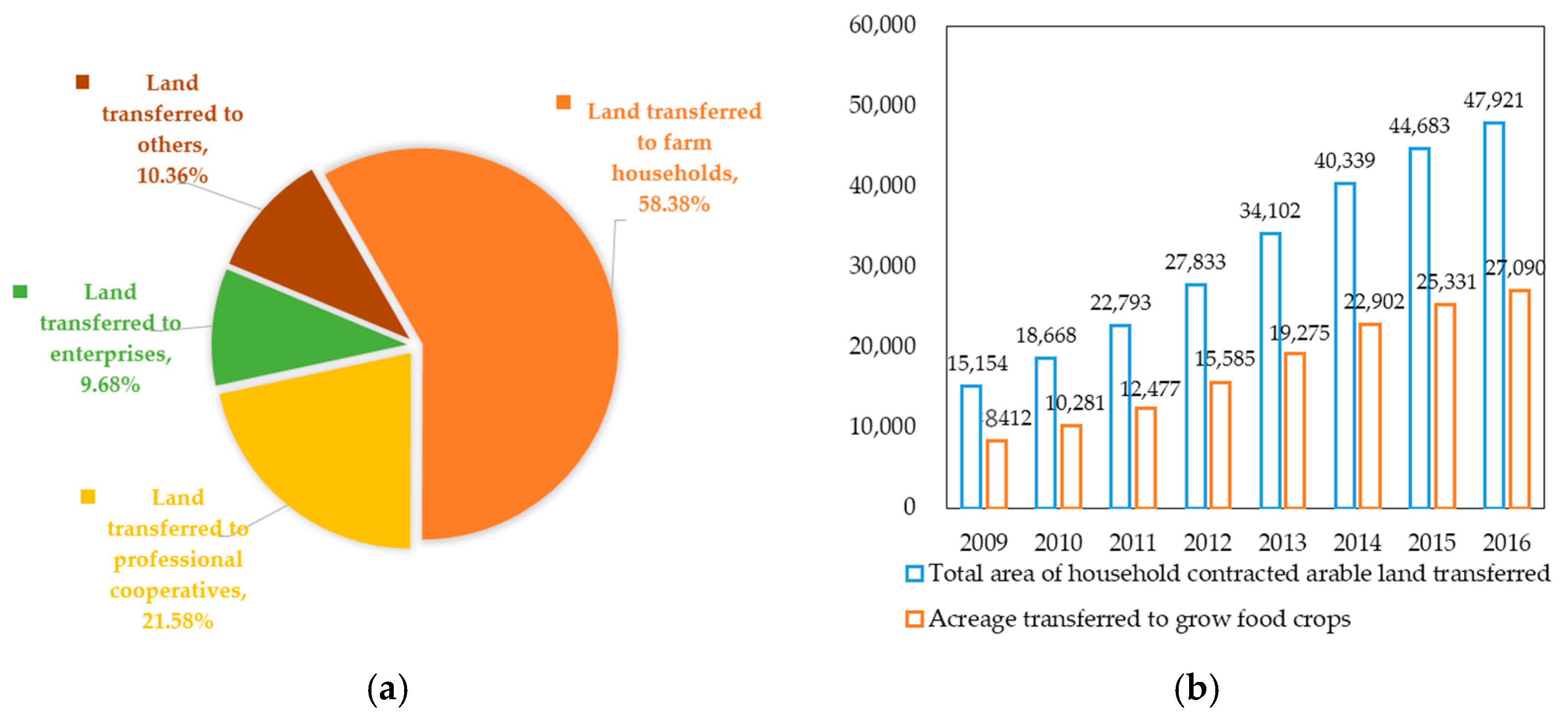
In China, land ownership lies with the state, but farmers have the right to contract and use the land. With the development of urbanization, the phenomenon of idle land is increasing. The Seventh Session of the Standing Committee of the 13th National People’s Congress voted and passed a decision on amending the Law on Rural Land Contracting. The main purpose of this revision of the Rural Land Contracting Law was to legalize the system for separating the ownership rights, contract rights, and management rights for contracted rural land. The ownership right, contract right and management right of land are separated. Farmers can freely choose to transfer the management right of land to others with compensation, which is referred to as land transfer in the article. This not only more effectively protects the legitimate rights and interests of farmers, also is but more conducive to the development of agricultural modernization. Transferring land is an important way to achieve large-scale agricultural operations. Because land has the dual functions of production and social security, it is necessary to understand decision-making behaviours regarding food production and the micro-mechanisms used by farmers before and after a land transfer, and understanding the impact of land transfers on food production efficiency and food security is especially important. Figure 1a,b reflect the accelerated land transfer rates in China in recent years and the number of farmers who have withdrawn from their land, respectively. As of 2016, the area of land that had been transferred had reached 35.14% of household-contracted arable land, and 30% of rural households had withdrawn from land planting. Figure 2a shows that 58.38% of the land that has been transferred is still held by small farm households, and 21.58% had been transferred to professional cooperatives. Figure 2b illustrates part of the trend towards non-grain farming. After transfer, 44% of the land is no longer used for growing food. Given such large-scale land transfers, along with the reorganization of agricultural business entities and the readjustment of the relationship between humans and land, what changes does land transfer have on the planting structure, production efficiency, and sustainable development of agriculture? Is the impact of land transfer on food production spatially heterogeneous? Answering these questions has great theoretical and practical significance for the sustainable development of agriculture, food security, and the efficient use of land.
The possible contributions of this article are as follows. Regional heterogeneity in land transfers is explored from a spatial perspective, the impact of land transfers on the grain planting structure as a micro-mechanism of farmers is explored, and the utility of land transfer due to income effects, scale effects, and structural effects is analysed. Using a multi-period heterogeneous difference-in-differences (DID) model, the problem of understanding land transfers among farmers at multiple points in time is better addressed.

2. Literature Review

Land and food security are inseparable. The effective use of land plays an important role in ensuring food security. Low efficiency in land use is an important obstacle to the realization of family welfare and national food security. There is a strong positive correlation between land scale and food production [1], and free land transfer is conducive to ensuring national food security [1,2,3]. The existing studies have mainly focused on the impact of land transfer on the outcomes such as grain production and economic crops.
Most scholars believe that land transfers are efficient [4,5,6,7,8,9,10,11,12,13,14,15,16,17,18,19,20,21,22], as they shift land from low-efficiency farmers to high-efficiency farmers [23,24,25,26]. The land lease market is not only conducive to the transfer of land from the less efficient to the more efficient but also conducive to the reallocation of land resources [27]. Land transfer increases productivity of labour, the productivity of agricultural tools, the productivity of agricultural assets, and the productivity of land, thereby increasing the efficiency of agricultural production [9,10,11]. Based on 2012 CFPS data, Qian Long found that transferring land among farmers significantly increased land productivity [28]. Zeng Yating used a transcendental logarithmic stochastic frontier production function to measure the technical efficiency of food production. Using a Tobit model to test for the factors influencing land transfer, it was found that land transfer improves the efficiency of food production technology by increasing the productivity of labour, agricultural tools, and agricultural materials but that it has a negative impact on land productivity [29]. Jin studied Kenyan household data and found that the land lease market can increase agricultural productivity [30]. In the process of urbanization, idle and abandoned land began to appear. During Japan’s rapid urbanization, farmland abandonment became a serious problem. Land rents and the rate of farmland abandonment were found to be negatively correlated [31]. Land transfer effectively uses idle land, thereby increasing agricultural productivity [12,13,14,15,16,17,18,32]. Koirala studied the impact of land ownership on the productivity and technical efficiency of Philippine rice farmers and found that the technical efficiency of farmers who transferred their land was higher than that of farmers who did not transfer land, which is consistent with the research conclusions of [33,34,35]. However, some scholars have explained the inefficiency in land transfers from other angles. With an increase in land rents, land transfers restrict improvements in agricultural production efficiency [36,37]; land transfers through government interventions are inefficient [38].
More economic crops are planted [39]. The planting structures of farmers who transfer land are susceptible to market forces and are more sensitive to the market. However, as the gap in the income earned from cash crops and food crops narrows, the impact of land transfers on planting structures should gradually weaken [40]. The main factors influencing non-grain planting behaviours related to land transfer are the age of the head of the household, the area of the cultivated land being worked, the proportion of non-agricultural income in total household income, the transfer rent and regional differences. However, some scholars have suggested that given the new land transfer situation, the planting structure is becoming oriented towards grain. The opportunity to maximize their income drives households engaged in small-scale farmland transfers to expand their cultivation of cash crops in order to increase their use of land and labour; however, with the transfer of rural labour to non-agricultural work and the rapid development of the agricultural services market, both of which have occurred to minimize the cost of farming, the return to a grain-oriented planting structure is the inevitable result [15,16].
The existing studies have examined the impact of land transfer on production efficiency, farmers’ income and agricultural inputs. This paper focuses on the farmers’ decision-making behaviour regarding production and the micro-mechanisms underlying those decisions and discusses the impact of land transfer on farmers’ planting structures and the spatial heterogeneity in those impacts. The innovations of this paper are to explore the regional heterogeneity in land transfer from a spatial perspective, to explore the impact of land transfer on the grain planting structure from the perspective of farmers, and to analyse the income effect, scale effect and structural effect of land transfers. The multi-period heterogeneous DID model solves the problem of farmers transferring land at multiple time periods.

3. Analysis of the Differences between Land Transfer and Food Planting

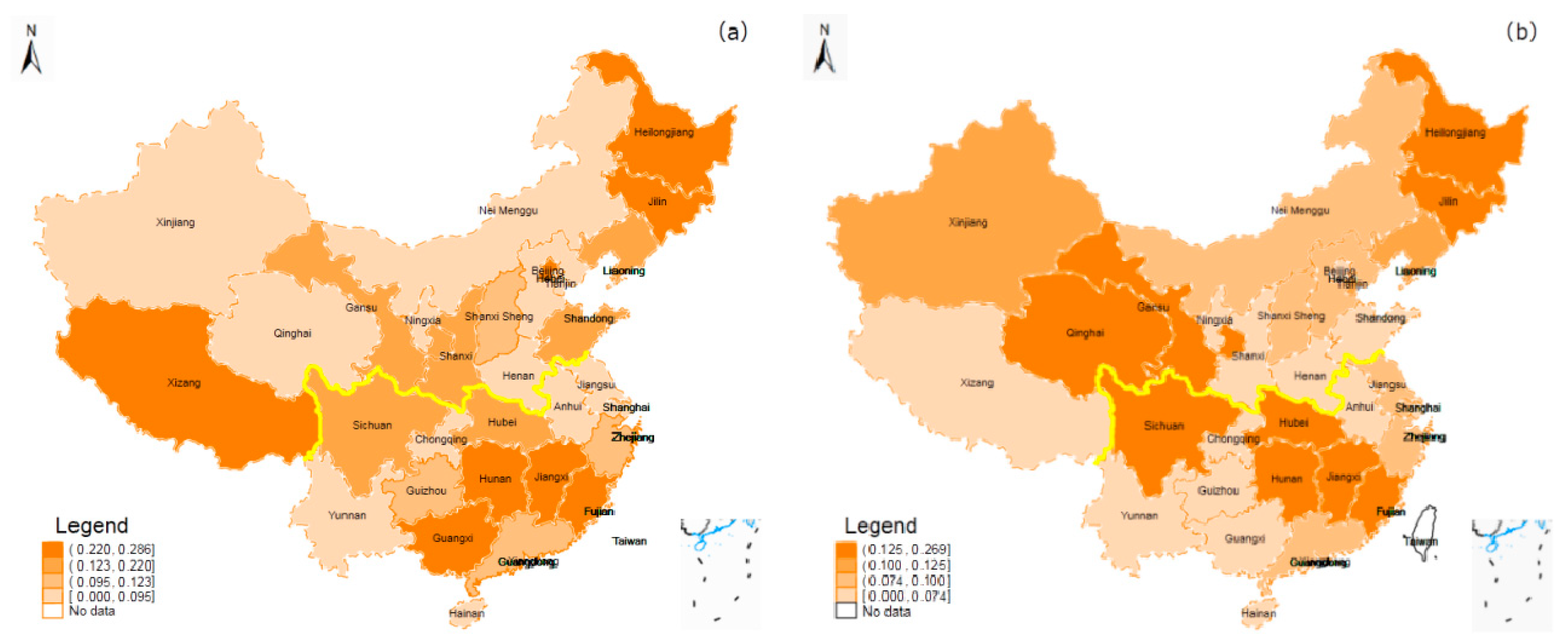
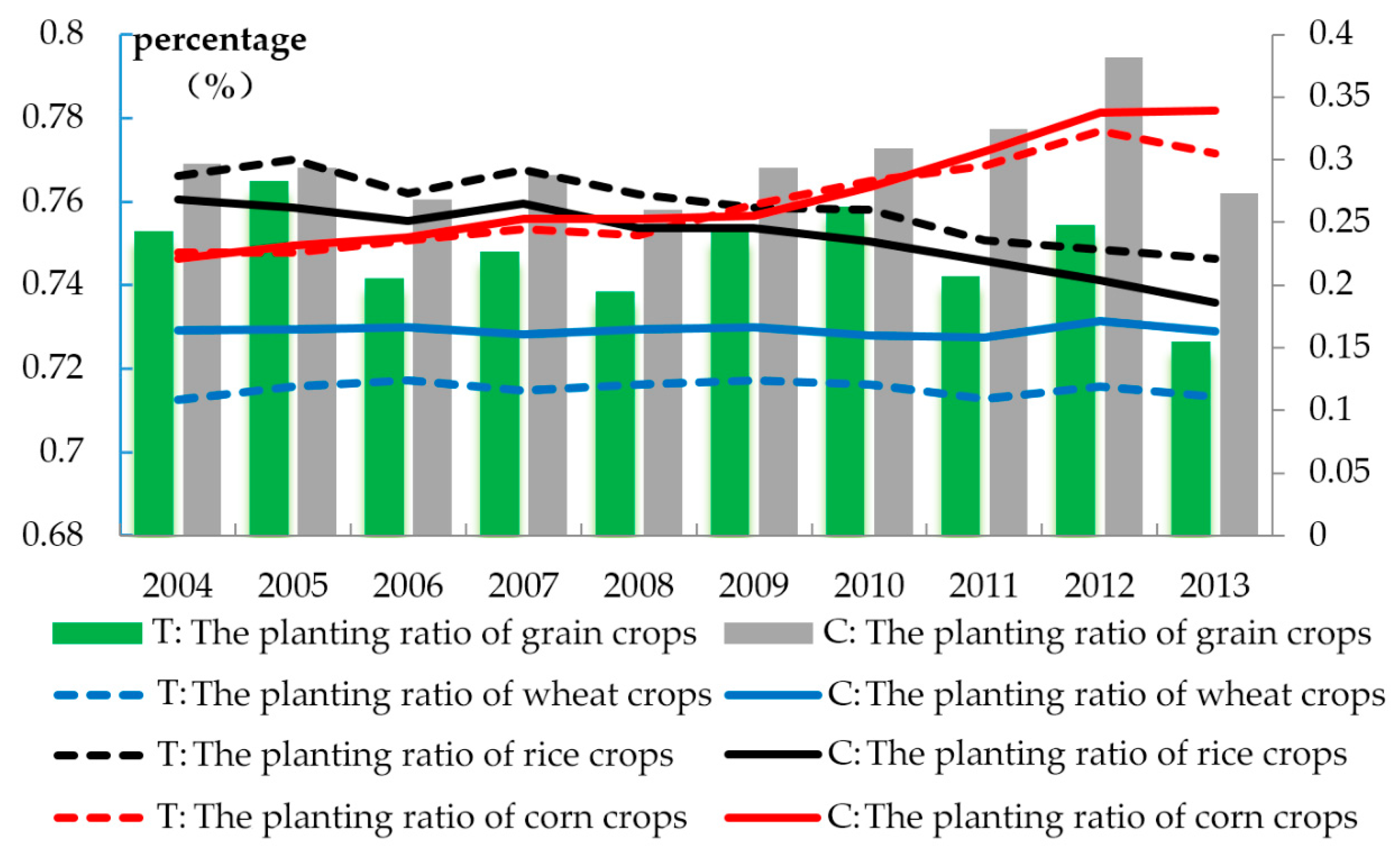
Figure 3 reflects the temporal and spatial changes in the land transfer rate among rural households in China, where the land transfer rate of rural households = households that have transferred land/(households that have transferred land + households that have not transferred land). In 2012, the darker the orange is, the higher the transfer rate among rural households. As shown in the figure, from 2004 to 2012, the transfer rate of rural households across the country increased, and the transfer rate of rural households in the northern region increased more quickly than that in the south. To analyse the impact of land transfer on grain planting structures, the observed households are divided into two groups: those that have transferred land and those that have not transferred land. Figure 4 shows that the proportion of grain planting and the proportion of wheat planting among households that have transferred land are continually lower than those of households that have not transferred land. However, the rice planting ratio among land transfer households is higher than that among non-transfer households. On the other hand, the proportion of grain planted is slowly decreasing (from 76.3% in 2004 to 74.8% in 2013), the proportion of corn planted increases overall, the proportion of rice planted has continued to decline slowly, and the proportion of wheat planted remains stable.
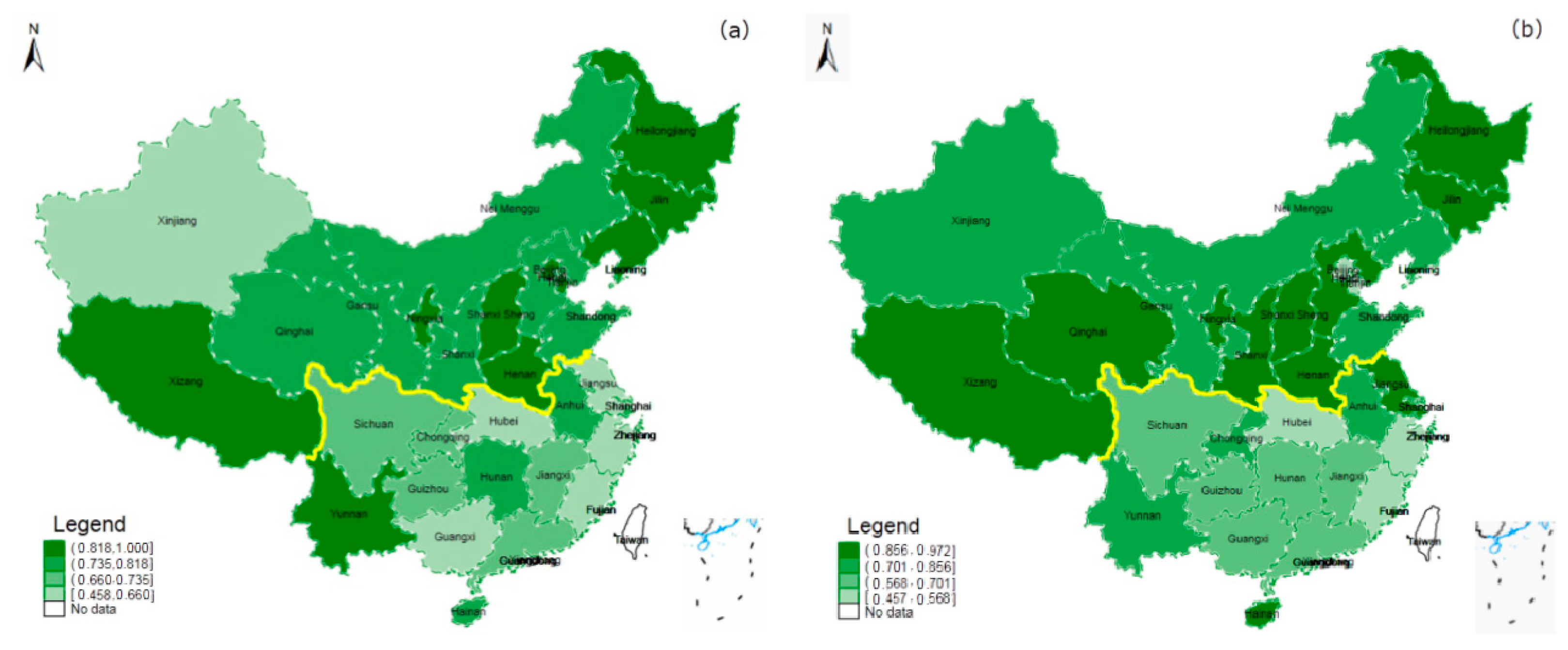
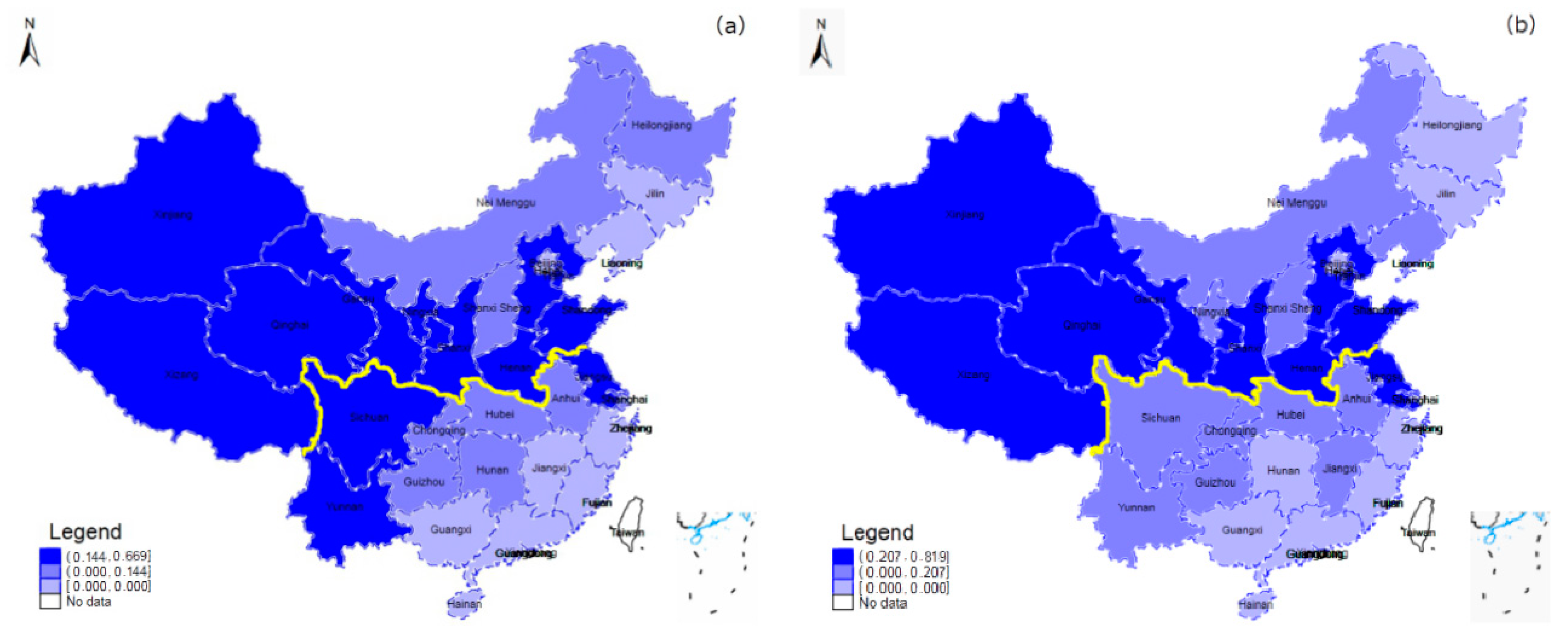
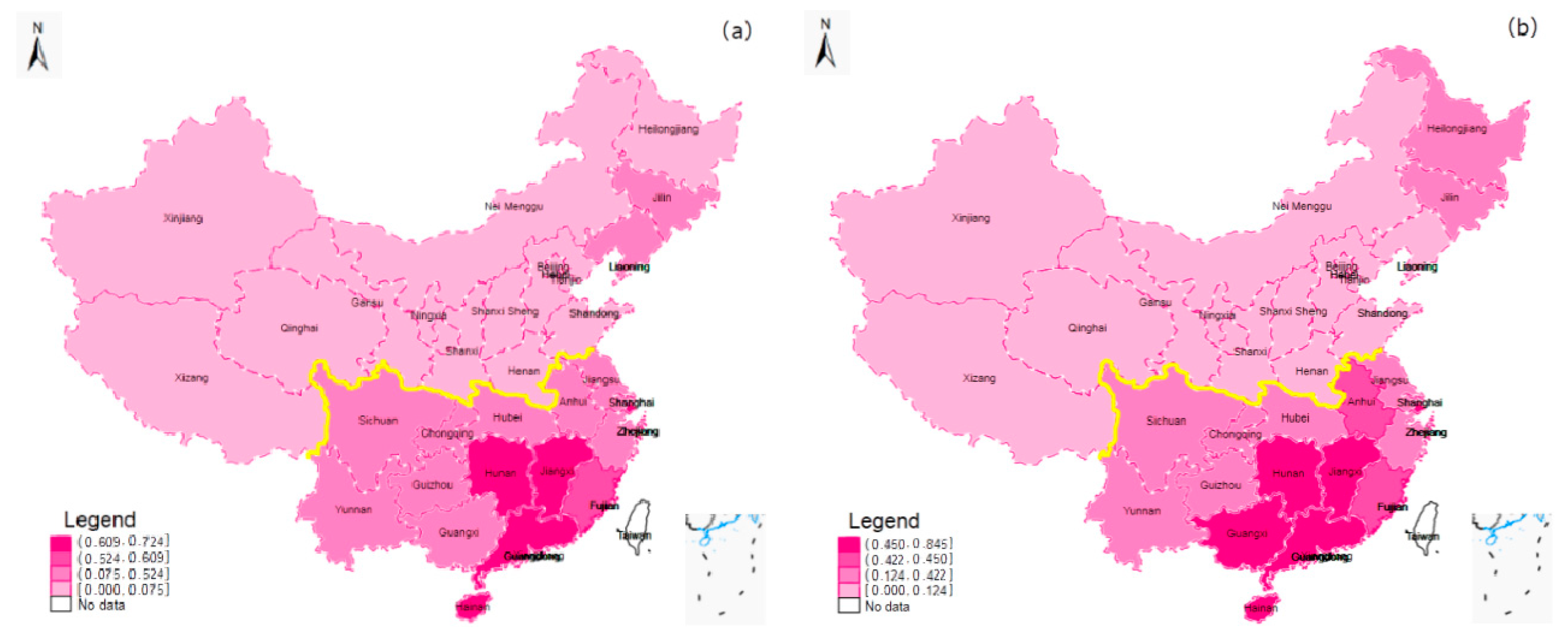
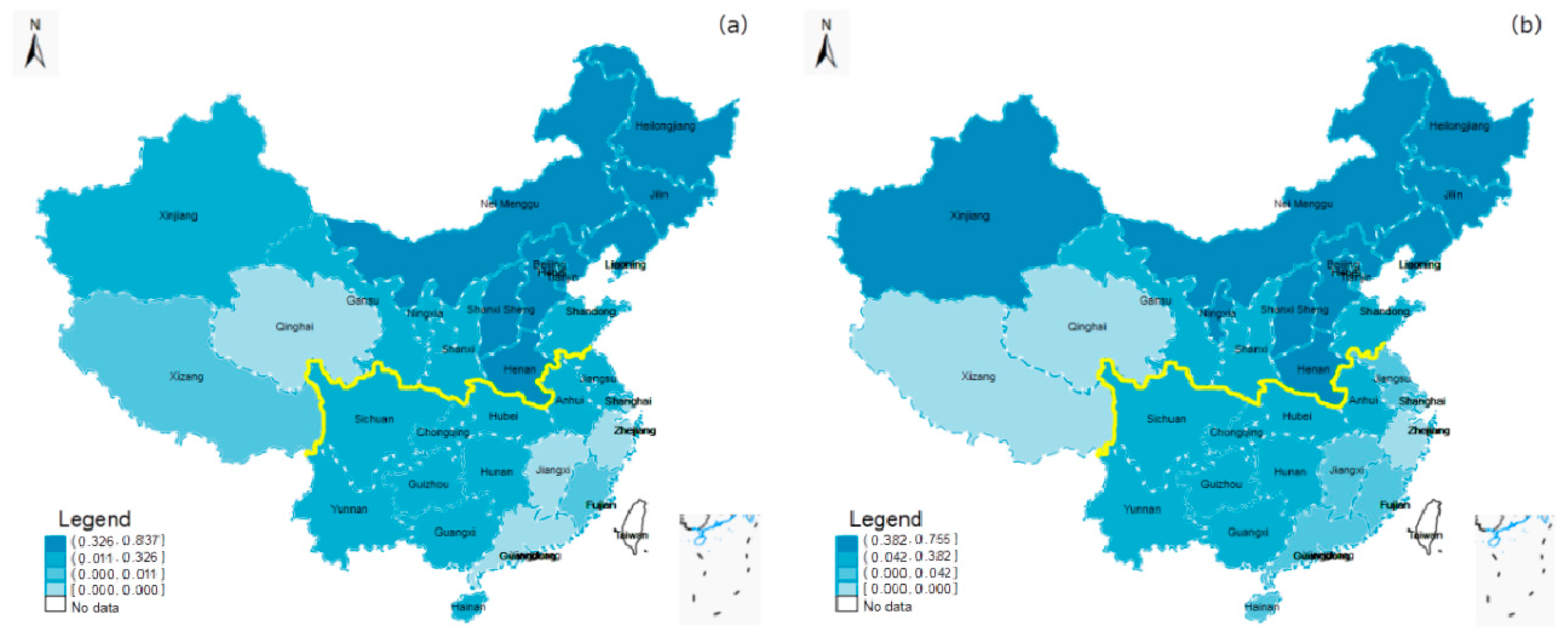
Based on the analysis of regional differences in the grain planting structure, panels a and b in Figure 5 show the distribution of the grain planting proportions in 2004 and 2012, respectively. The darker the green colour is, the higher the proportion of grain planted. The grain planting ratio has declined, but the agricultural planting structure in the north is more grain-oriented than that in the south. The yellow line in the figure represents the dividing line between the north and the south. The regions included in the north and south are as follows. The area north of the yellow line includes Heilongjiang Province, Xinjiang Uygur Autonomous Region, Jilin Province, Liaoning Province, Inner Mongolia Autonomous Region, Tibet Autonomous Region, Beijing, Ningxia Hui Autonomous Region, the city of Tianjin, Hebei Province, Henan Province, Qinghai Province, Shaanxi Province, Shandong Province, Gansu Province, and Shanxi Province. The area south of the yellow line includes Hainan Province, Guangdong Province, Taiwan Province, Hong Kong Special Administrative Region, Macao Special Administrative Region, Yunnan Province, Guangxi Zhuang Autonomous Region, Guizhou Province, Jiangxi Province, Fujian Province, Jiangsu Province, Anhui Province, Hunan Province, Hubei Province, Sichuan Province, the city of Chongqing, Shanghai, and Zhejiang Province. In terms of the grain varieties planted, Figure 6, Figure 7 and Figure 8 show the temporal and spatial changes in the planting ratios for wheat, rice, and corn, respectively. The figure shows that as of 2012, the grain planting pattern of rice in the south and wheat in the north was basically determined, while the ratio of corn planting did not vary significantly across time or space.

4. Variables and Models

4.1. Description of Data and Variables

The data used in this article are the micro-level data from 2004 to 2013, which are from the panel survey data of fixed rural observation points from Chinese Ministry of Agriculture covering 31 provinces. The total sample size is 13,626 households, with 6691 households in the southern region and 6935 households in the northern region. Part of the macro-level data used comes from the “China Agricultural Development Reports” from 2009 to 2017.
In addition to the core explanatory variable, land transfer, four categories of factors are defined that affect agricultural production: the characteristics of the head of the household, the characteristics of the family’s labour force, the factors related to family agricultural operations, and the extent of agricultural development at the provincial level.
The variables related to the head of household include the age of the head of household, the sex of the head of household, the educational level of the head of household, and the agricultural training status of the head of household. As the decision-maker for household management, the age, sex, education level, and training of the head of household are expected to significantly affect the decision to transfer land, family income, and the crops planted.
The characteristics of the family labour force include the size of the family labour force, the average age of the members of the family labour force, the average years of education among members of the family labour force, and the average health level among members of the family labour force. These variables are used to control for the influence of family labour force characteristics. The health of the family labour force is also a standard measure of the family’s ability to engage in agriculture.
The family management module includes arable land area under household management, the degree of land fragmentation, and the value of the productive fixed assets owned by the family. The scale of household management is related not only to whether farmers are willing to transfer land, but also to the household’s planting structure, agricultural income, and agricultural efficiency. The degree of land fragmentation not only captures the characteristics of China’s existing cultivated land but also reflects the trends in the agricultural scale in China. The value of the productive fixed assets owned by families can be used to measure the degree to which production has been mechanized.
The regional control variables include the proportion of the primary industry to the GDP of the whole province, the per capita land area of the province, the per capita GDP of the province, the cultivated land resources in the province, and the total provincial investments into the primary industry, which are used to measure the level of agricultural development in each province. To an extent, the provincial-level per capita land area, per capita GDP, and cultivated land resources explain the resources available for the development of the primary industry. Because China has a vast territory, the distribution of resources and population among provinces is very uneven. Controlling for these variables helps eliminate estimation bias in the results to a certain extent.
When the effect of land transfer on farmers’ welfare is studied, most scholars use household income as the welfare measure. In this paper, we use household agricultural management income as an explanatory variable to capture the income effect. The scale effect is the increase in efficiency or the reduction in costs that occurs when the scale of operations increases. Therefore, the yield per unit area of agricultural crops and the average fertilizer cost per unit area of agricultural crops are used to identify whether there are scale effects.
The dependent variables studied in this article are structured to allow for two analyses, namely, an analysis of the structural effect of land transfer and utility analysis of that structural effect. The measurement indicators for the structural effect include the proportion of grain planted, the wheat planting proportion, the rice planting proportion, and the corn planting proportion; the utility analysis of the structural effect includes the per unit area yield of grain crops, the input–output ratio, household agricultural business income, and total household income. See Table 1.
The variables affecting agricultural production can be divided into two categories, namely, the core explanatory variables and the control variables. The core explanatory variable is a dummy variable for whether the land has been transferred; the control variables consist of four categories. The first category includes the household head characteristics, including sex, age, education level, and the agricultural training of the household head, and the second category includes the family labour force characteristics, including the size, average age, average education level, and average self-reported health status of the family labour force. The third category of control variables covers the status of the family agricultural business, including the scale of operations, the degree of land fragmentation, and the value of any productive fixed assets. The fourth category includes the characteristics of the province, including the proportion of the primary industry, the province’s population density, its economic density, its arable land resources, and the government’s investment into the primary industry. See Table 2.

4.2. Methods and Models

In this article, the land circulation is a kind of public policy, and the difference in agricultural production between households that participate and those that do not participate in land transfer is affected by many factors. Then, land transfer can be seen as a quasi-natural experiment, which meets the basic framework of counterfactual analysis. Therefore, the widely used DID model can be used to evaluate the policy effect, which can make a more realistic evaluation of the implementation effect of land transfer. The traditional DID assumes that all individuals are affected by policies at the same time. However, in this paper, due to the different years in which land transfer occurred among farmers, that is, the individual policy impact time is different, the multi-period DID model needs to be applied even more at this time. At this point, the metrological equation can be briefly expressed as:
Y i t = 1 + 2 × t r e a t i × p o s t i t + c t + c i + σ .
The method evaluates the change of the observed variables (dependent variable) under the two situations of whether or not to transfer land. Therefore, the samples are divided into the experimental group ( t r e a t i = 1 ) and the control group ( t r e a t i = 0 ). p o s t i t represents the processing state of individual I at time t. If the land is transferred, p o s t i t is 1; otherwise, it is 0. Therefore, farmers can incur interference from policies at different time points in the model setting. The coefficient of cross-product term 2 is the average treatment effect under consideration in this paper. Equation (2) shows the calculation principle of the average treatment effect expressed by the coefficient 2 and reflects the difference between the treatment group and the control group before and after the farmers’ land transfer in terms of their planting behaviour
           2 = { E [ Y i t | t r e a t i = 1 , p o s t i t = 1 ] E [ Y i t | t r e a t i = 1 , p o s t i t = 0 ] }                         { E [ Y i t | t r e a t i = 1 , p o s t i t = 1 ] E [ Y i t | t r e a t i = 1 , p o s t i t = 0 ] } = ( Y 1 Y 0 ) ( C 1 C 0 ) = ( 2 + c t ) c t = ( Y 1 C 1 ) ( Y 0 C 0 ) = ( 2 + c i ) c i
Furthermore, the cross-product term t r e a t i × p o s t i t in Equation (1) is equivalent to the dummy variable t r e a t e d i , which represents the treatment of individual i at time t. Therefore, by using t r e a t e d i to simplify Equation (1) and introducing control variables, the econometric estimation equation in this paper can be set as Equation (3):
Y i = 1 + 2 × t r e a t e d i + n 1 3 n × D n i + c t + c j + σ .
In this paper, households that have transferred land in since 2004 are classified into the treatment group; that is, for the households that have transferred land in, the value of the corresponding treatment variable is recorded as 1. The households that have not transferred land in between 2004 and 2013 are classified as the control group; that is, for the households that have not transferred land in, the value of the corresponding treatment variable is recorded as 0. In this paper, the sample of farmers who have transferred land out are excluded from the empirical research. In addition, Y i is measured as the proportion of the cultivated area sown with grain, with wheat, with rice, and with corn for the i-th agricultural household in Equation (3). Additional dependent variables include the i-th farmer’s household operating income and total income, as well as the yield per unit area and input–output ratio of the i-th farmer’s food crops. The variable t r e a t e d i indicates whether the i-th farmer has transferred land in; if so, the variable is equal to 1, while it is 0 for farmers who have not. D n i represents the control variables, which includes the characteristics of the head of the i-th agricultural household, including age, sex, education level, and agricultural training status; the characteristics of the family labour force of the i-th agricultural household, including the size of the household labour force, the average age of members of the household labour force, the average education level of the members of the household labour force, and the average health status of the members of the household labour force; the family business characteristics of the i-th agricultural household, including the scale of operations, the degree of land fragmentation, and the value of the agricultural fixed assets; and the characteristics of the province in which the i-th agricultural household resides, including population density, economic density, the total arable land area of the province, and total agricultural investment in the province. The variables c t and c i represent year and village effects, respectively; σ is a constant, and 1 ~   3   are the coefficients to be estimated.
Equation (3) needs to control the individual and time effects, so this paper mainly adopts a panel fixed-effects model. The panel fixed-effects model is conducive to removing unobserved variables that do not change over time, helps reduce endogeneity, and can generate robust estimation results. Additionally, because we cannot ensure that the assumption that the random error term is not related to the core explanatory variables is satisfied, the panel fixed-effects model is used for the empirical analysis. This paper uses the survey data of fixed rural observation points from Chinese Ministry of Agriculture from 2004 to 2013, and it rejects the null hypothesis according to the results of the Hausman test shown in Table 3, which also supports the use of the panel fixed-effects model.

5. Analysis of the Empirical Results

We use the ratios of food crops, of wheat, of rice, and of corn as dependent variables to empirically determine whether land transfer causes changes in the grain production structure. To better control for endogeneity, time fixed effects and village fixed effects are used. Basic results are reported in Table 4.
The empirical results presented in Table 4 show that land transfer has changed the crop planting structure, resulting in a decrease in grain planting, which is specifically manifested in the negative impact of land transfer on the share of the three staple foods being planted; that is, land transfer has reduced the shares of wheat, rice and corn that farmers plant, and thus, as a result, the proportion of grain planted has declined. In the regression of food crop planting on the ratio of land transfer, a further increase in the control variables did not change the sign or significance of the coefficient. In addition, the regression results show that reducing the degree of land fragmentation, increasing the value of the productive fixed assets owned by farmers, and strengthening the government’s emphasis on and investment in agriculture helps increase food planting.
To verify whether there is regional heterogeneity in the impact of land transfer on the planting structure of farmers, the southern and northern subsamples were analysed. The empirical results presented in Table 5 show that land transfer has a negative effect on the grain planting structure in both the southern and northern regions. Compared with that in the northern region, the impact of land transfer on the shift away from planting grain crops is more obvious in the southern region.
To investigate the impact of land transfer on grain production efficiency and farmers’ income, grain yield per unit area and the grain input–output ratio were used to measure the efficiency of farmers’ grain production, while time fixed effects and village fixed effects were used. The empirical regression results for model 1 and model 2 in Table 6 show that land transfer has no significant impact on grain production efficiency, but the empirical results for model 3 in Table 6 show that land transfer increases household operating income.
The results for model 1 and model 4 in Table 7 are consistent with those in Table 6. The land transfer has no impact on grain production efficiency. Model 5 and model 6 examine the north–south differences in the impact of land transfer on agricultural operating income. The empirical results show that the effect of land transfer on household agricultural income in the southern region is less than that in the northern region, which may be related to differences in the degree of land fragmentation and land transfer regulations in the north and south.

6. Robustness Test

6.1. Robustness Test: Differences-in-Differences

The largest difference between the DID model and the previously used model setting is that there is an additional dummy variable, time, indicating when the policy occurs. In this paper, the year after land transfer occurs is recorded as 1 for the time variable, and for the year before land transfer occurs, the time variable is set to 0. The model is set as follows:
Y i = 1 + 2 × t r e a t e d i × t i m e i + n 1 3 n × D n i + c t + c j + σ .
Except for the inclusion of an additional event dummy variable, the other variables and parameter settings are consistent with those in formula (1). Here, timei represents the dummy variable for the i-th farmer’s land transfer.
The above three outcomes for the impact of land transfer on agricultural production are regressed using the DID model. The dependent variables used are consistent with those from the first three analyses, but the model construction is changed to that of Equation (2). The core explanatory variable becomes treatedi × timei, namely, the DID variable.
The robust results of the DID model for the impact of land transfer on the planting structure of farmers and the utility analysis are shown in Table 8, Table 9 and Table 10. In comparison to previous estimation results, the basic conclusions are consistent, verifying that the empirical results are robust.

6.2. Robustness Test: Changing the Time Window

The time span of the panel data was changed from 2004–2013 to 2006–2011, and the DID regression was re-conducted to test the robustness of the estimation results. The results of the robustness test with the changed time window (see Table 11, Table 12 and Table 13), except for the change in the sign of the coefficient for land transfer’s impact on the per unit area fertilizer input of food crops, are consistent with the original estimation results. They show that land transfer has a significant structural effect on farmers’ grain planting behaviour, and there are also differences regarding the north and the south. Moreover, the non-grain cultivation is more obvious in the south, while the income effect of land transfer is more obvious in the north. The different result for fertilizer input may be the result of expenses not being deflated. Therefore, the above two robustness tests, the DID regression, and the change of the time window yielded estimation results consistent with the previous results in this article, which further strengthens the credibility of the empirical conclusions.

7. Conclusions and Recommendations

This article uses the survey data of fixed rural observation points provided by Chinese Ministry of Agriculture from 2004 to 2013 to explore the north–south differences in the impact of land transfer on farmers’ food planting and to analyse the impact of land transfer on food production in terms of structure and efficiency using a multi-period heterogeneous difference-in-differences model and the propensity score matching technique. The empirical research conclusions are as follows:
(1)
Land transfer reduces the planting of food crops and leads farmers to shift to the planting of cash crops.
(2)
There is regional heterogeneity in the impact of land transfers on the grain planting structure. The shift away from planting grains is more prominent in the south than in the north. Land transfer reduced wheat cultivation in the north and rice cultivation in the south.
(3)
Land transfer has increased the operating income of farmers, and the income of farmers in the north is higher than that in the south.
(4)
Land transfer among farmers is mainly small-scale transfer, which does not improve the efficiency of farmers’ grain planting.
Given the process of urbanization, the transfer of the agricultural labour force to cities, and the ageing of the agricultural labour force, land transfers and agricultural modernization are the only ways to ensure food security and promote sustainable agricultural development. First, we must take the shift away from grain cultivation in the process of land transfer seriously to ensure food security. On the other hand, it is necessary to establish a market mechanism for land transfers, explore effective business models to guide capital to rural areas, and promote the appropriate scale of land transfer and the development of modern agriculture. Second, in terms of the different effects of urbanization in the northern and southern regions, the southern region has a more developed economy and more non-agricultural employment opportunities. The transfer of grain from the south to the north shows that the regional division of labour and the grain planting structure are affected by urbanization, and the north and south should be monitored differently. An increased scale of land transfer and additional shifts in the grain planting structure are expected to strengthen the regional division of labour and these structural adjustments. Therefore, policymakers should catch the dividend express of the digital economy by developing digital agriculture and smart agriculture, using technology to promote the development of agriculture, rural areas, and farmers, innovating land transfer models, and improving grain planting efficiency.
Because the latest data are not available, this paper cannot track the latest land transfer changes, which is the most substantial limitation of this paper. On the other hand, since the data are based on the sample of farmers, the lack of corporate data cannot reflect the situation of large-scale land circulation. In future work, the land inflow operation behaviour of agricultural companies of a certain scale will be separately studied.

Author Contributions

Conceptualization, Z.L. and X.H.; methodology, Y.W. and X.H.; resources, Z.L.; data curation, Y.W. and Z.L.; writing—original draft preparation, Z.L. and Y.W.; writing—review and editing, Z.L. and X.H.; supervision, Z.L. and X.H.; funding acquisition, Z.L. All authors have read and agreed to the published version of the manuscript.

Funding

This research was funded by the National Social Science Foundation of China, grant number 16BJY105.

Institutional Review Board Statement

Not applicable.

Informed Consent Statement

Not applicable.

Data Availability Statement

The data presented in this study are available on request from the corresponding author, while restrictions may apply to the availability of the APM data.

Conflicts of Interest

The authors declare no conflict of interest.

References

  1. Shang, X.; Zhu, S. Analysis on the effect of agricultural land transfer subsidy policy—Based on crowding out effect, government rent creation and target deviation. China Rural Obs. 2017, 6, 43–56. [Google Scholar]
  2. Zhai, L.; Xia, X.; Wu, A. The impact of farmland transfer on Farmers’ livelihood capital under different government intervention scenarios: An econometric analysis based on psm-did. China Rural Econ. 2017, 2, 2–15. [Google Scholar]
  3. Pranay, R.; Chloe, B.W.; Francis, R.E.; Sheila, M.W.R.; Linda, S.P. Understanding barriers and opportunities for adoption of conservation practices on rented farmland in the US. Land Use Policy 2019, 80, 214–223. [Google Scholar]
  4. He, X.; Jiang, T.; Guo, L.; Gan, L. Research on the development of China’s farmland transfer market and farmers’ Farmland Transfer Behavior—Based on the survey data of 29 provinces from 2013 to 2015. Manag. World 2016, 6, 79–89. [Google Scholar]
  5. Zhu, W.; Luo, B. Farmland price illusion: The “failure” of farmland transfer market allocation caused by the difference of value evaluation—Based on the micro data of farmers in 9 provinces (regions) in China. China Rural Obs. 2018, 5, 67–81. [Google Scholar]
  6. Tian, C.; Fang, L. Land adjustment and farmland leasing market: A dual perspective based on quantity and quality. Econ. Res. 2013, 48, 110–121. [Google Scholar]
  7. Wang, Y.; Li, X.; Li, W.; Tan, M. Land titling program and farmland rental market participation in China: Evidence from pilot provinces. Land Use Policy 2018, 74, 281–290. [Google Scholar] [CrossRef]
  8. Xu, Z.; Tan, X.; Zheng, X.; Lu, W. Influence and constraint conditions of farmland transfer market development on grain production. China Rural Econ. 2017, 9, 26–43. [Google Scholar]
  9. Gao, L.; Huang, J.; Rozelle, S.; Xu, Z. The development of China’s farmland transfer market and its impact on Farmers’ Investment. Economics 2011, 10, 1499–1514. [Google Scholar]
  10. Heidi, L.; Marianne, P.; Klaus, S. Do farmers care about rented land? A multi-method study on land tenure and soil conservation. Land Use Policy 2019, 82, 228–239. [Google Scholar]
  11. Ma, X.; Qiu, T.; Qian, Z. Security of farmland property rights and farmers’ participation in farmland transfer market: An Empirical Analysis Based on survey data of Jiangsu, Hubei, Guangxi and Heilongjiang provinces. China Rural Econ. 2015, 2, 22–37. [Google Scholar]
  12. Lin, W.; Qin, M.; Su, Y.; Wang, Z. How does the new round of farmland ownership affect farmland transfer?—Evidence from China’s health and pension follow-up survey. China Rural Econ. 2017, 7, 29–43. [Google Scholar]
  13. Xu, Q.; Liu, J.; Qian, Y. Labor mobility, farmland ownership and farmland transfer. Agric. Technol. Econ. 2017, 5, 4–16. [Google Scholar]
  14. Luo, M.; Xu, Q.; Lu, Y. Non agricultural employment, social security function of land and farmland transfer. China Popul. Sci. 2018, 5, 30–41, 126–127. [Google Scholar]
  15. Luo, B. Coase Theorem: Reflection and expansion: On the reform and selection of China’s farmland transfer system. Econ. Res. 2017, 52, 178–193. [Google Scholar]
  16. Qiu, T.; Luo, B. Will farmland adjustment inhibit the non-agricultural transfer of rural labor force? China Rural Obs. 2017, 4, 57–71. [Google Scholar]
  17. Wang, Q.; Ren, Q.; Yu, J. Empirical analysis on the bargaining power of farmers in major grain producing areas. China Rural Obs. 2018, 2, 47–59. [Google Scholar]
  18. Ayala, W.; Thomas, S.J. Land Prices Heading Skyward? An Analysis of Farmland Values across Tanzania. Appl. Econ. Perspect. Policy 2018, 40, 187–214. [Google Scholar]
  19. Li, T.; Zhao, Y.; Xin, X. Analysis of basic characteristics and influencing factors of current farmland transfer. China Rural Econ. 2009, 10, 4–11. [Google Scholar]
  20. Hou, J.; Huo, X. Credit availability, financing scale and farmers’ Farmland Transfer: A case study of specialized farmers. China Rural Obs. 2016, 6, 29–39. [Google Scholar]
  21. Ani, L.K.; Mary, C.A. Dynamics of Farmland Ownership and Leasing: Implications for Young and Beginning Farmers. Appl. Econ. Perspect. Policy 2016, 38, 334–350. [Google Scholar]
  22. Su, L.; He, X.; Kong, R. The impact of financial knowledge on Farmers’ Farmland Transfer Behavior: An analysis based on the regulatory effect of farmland confirmation certificate. China Rural Econ. 2018, 8, 17–31. [Google Scholar]
  23. TrieuHuy, H.; ThanhNguyen, T. Cropland rental market and farm technical efficiency in rural Vietnam. Land Use Policy. 2019, 81, 408–423. [Google Scholar]
  24. Deininger, K.; Jin, S. The potential of land rental markets in the process of economic development: Evidence from China. J. Dev. Econ. 2005, 78, 241–270. [Google Scholar] [CrossRef]
  25. Tan, S.; Zhang, R.; Tan, Z. Grassland rental markets and herder technical efficiency: Ability effect or resource equilibration effect? Land Use Policy 2018, 77, 135–142. [Google Scholar] [CrossRef] [Green Version]
  26. Chen, H.; Shi, Q.; Gu, H. Is rural land transfer efficient? Taking Shanxi as an example. China Rural Econ. 2014, 7, 61–71. [Google Scholar]
  27. Chamberlin, J.; Ricker-Gilbert, J. Participation in Rural Land Rental Markets in Sub-Saharan Africa: Who Benefits and by How Much? Evidence from Malawi and Zambia. Am. J. Agric. Econ. 2016, 98, 1507–1528. [Google Scholar] [CrossRef] [Green Version]
  28. Qian, L.; Hong, M. Non agricultural employment, land transfer and agricultural production efficiency change: An Empirical Analysis Based on CFPS. China Rural Econ. 2016, 12, 2–16. [Google Scholar]
  29. Zeng, Y.; Lv, Y.; Liu, W. Does farmland transfer improve the technical efficiency of grain production—From the perspective of farmers. Agric. Technol. Econ. 2018, 3, 41–55. [Google Scholar]
  30. Jin, S.; Jayne, T.S. Land Rental Markets in Kenya: Implications for Efficiency, Equity, Household Income, and Poverty. Land Econ. 2013, 89, 246–271. [Google Scholar] [CrossRef]
  31. Ito, J.; Nishikori, M.; Toyoshi, M.; Feuer, H.N. The contribution of land exchange institutions and markets in countering farmland abandonment in Japan. Land Use Policy 2016, 57, 582–593. [Google Scholar] [CrossRef]
  32. Jin, S.; Deininger, D. Land rental markets in the process of rural structural transformation: Productivity and equity impacts from China. J. Comp. Econ. 2009, 37, 629–646. [Google Scholar] [CrossRef] [Green Version]
  33. Feng, S.; Heerink, N.; Ruben, R.; Qu, F. Land rental market, off-farm employment and agricultural production in Southeast China: A plot-level case study. China Econ. Rev. 2010, 21, 598–606. [Google Scholar] [CrossRef]
  34. Feng, S. Land rental, off-farm employment and technical efficiency of farm households in Jiangxi Province. China. NJAS Wagening. J. Life Sci. 2008, 55, 363–378. [Google Scholar] [CrossRef] [Green Version]
  35. Koirala, K.H.; Mishra, A.; Mohanty, M. Impact of land ownership on productivity and efficiency of rice farmers: The case of the Philippines. Land Use Policy 2016, 50, 371–378. [Google Scholar] [CrossRef]
  36. Liu, Y.; Yan, B.; Wang, Y.; Zhou, Y. Will land transfer always increase technical efficiency in China?—A land cost perspective. Land Use Policy 2019, 82, 414–421. [Google Scholar] [CrossRef]
  37. Deininger, D.; Jin, S.; Nagarajan, H.K. Efficiency and equity impacts of rural land rental restrictions: Evidence from India. Eur. Econ. Rev. 2008, 52, 892–918. [Google Scholar] [CrossRef] [Green Version]
  38. Wang, X.; Cao, T.; Zou, W. Impact of local government intervention on agricultural land transfer on production efficiency: An analysis based on rice growers. China Popul. Resour. Environ. 2018, 28, 133–141. [Google Scholar]
  39. Yi, X.; Chen, Y. Analysis on Influencing Factors of farmers’ transfer to cultivated land and their “non grain” planting behavior and scale—Based on the survey data of farmers in Zhejiang and Hebei provinces. China Rural Obs. 2010, 6, 2–10. [Google Scholar]
  40. Wang, T.; Luri, M.; Janssen, L.; Hennessy, D.A.; Feng, H.; Wimberly, M.C.; Arorae, G. Determinants of Motives for Land Use Decisions at the Margins of the Corn Belt. Ecol. Econ. 2017, 134, 227–237. [Google Scholar] [CrossRef] [Green Version]
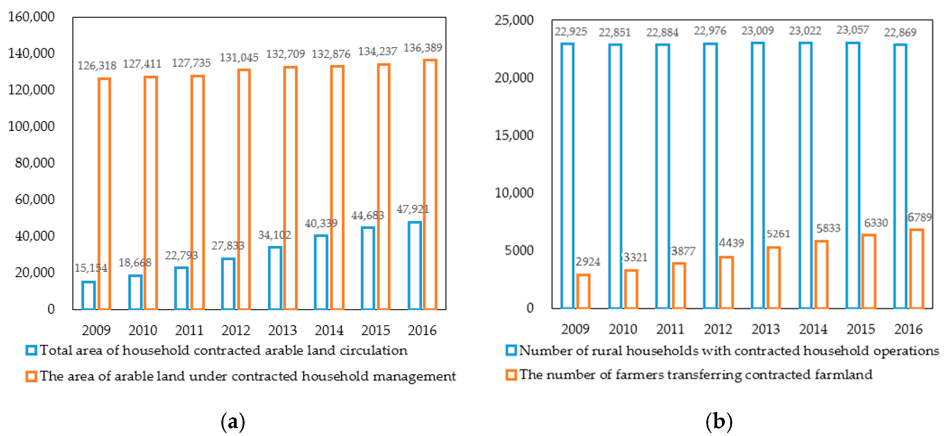
Figure 1. (a) Land transfer area of rural households from 2009 to 2016 (unit: ten thousand mu (mu, a Chinese unit of land measurement which is commonly 666.7 square meters)); (b) Number of rural households who transferred land from 2009 to 2016 (unit: ten thousand households).
Sustainability 13 03327 g001
Figure 2. (a) The structure of land transfer in 2016; (b) The acreage used to grow food crops after land transfer. Data source: Ministry of Agriculture “China Agricultural Development Report”.
Sustainability 13 03327 g002
Figure 3. (a) Land transfer rate of rural households in 2004; (b) Land transfer rate of rural households in 2012. Note: The area above the yellow line is the north, including Heilongjiang Province, Jilin Province, Liaoning Province, Inner Mongolia Autonomous Region, Beijing, Tianjin, Hebei Province, Henan Province, Shandong Province, Xinjiang Uygur Autonomous Region, Tibet Autonomous Region, Gansu Province, Qinghai Provinces, Ningxia Hui Autonomous Region, Shaanxi Province, and Shanxi Province; the area below the yellow line is the south, including Hainan Province, Guangdong Province, Taiwan Province, Hong Kong Special Administrative Region, Macao Special Administrative Region, Yunnan Province, Guangxi Zhuang Autonomous Region, Guizhou Province, Jiangxi Province, Fujian Province, Jiangsu Province, Anhui Province, Hunan Province, Hubei Province, Sichuan Province, Chongqing City, Shanghai, and Zhejiang Province.
Sustainability 13 03327 g003
Figure 4. The planting ratio of grain crops, wheat, rice, and corn crops of households that have transferred land and those that have not transferred land. Data source: Survey data of fixed rural observation points from Chinese Ministry of Agriculture. Note: T means households that have transferred land; C means households that have not transferred land.
Sustainability 13 03327 g004
Figure 5. (a) Grain planting ratio in 2004; (b) Grain planting ratio in 2012. Data source: Survey data of fixed rural observation points from Chinese Ministry of Agriculture.
Sustainability 13 03327 g005
Figure 6. (a) Wheat planting ratio in 2004; (b) Wheat planting ratio in 2012.
Sustainability 13 03327 g006
Figure 7. (a) Rice planting ratio in 2004; (b) Rice planting ratio in 2012.
Sustainability 13 03327 g007
Figure 8. (a) Corn planting ratio in 2004; (b) Corn planting ratio in 2012.
Sustainability 13 03327 g008
Table 1. Definition and descriptive statistics of dependent variables.
VariablesVariable DescriptionMeanStd.MinMax
cropperSown area of food crops/sown area of food crops + sown area of cash crops0.770.3001
xiaomaiperWheat sown area/food crop sown area + cash crop sown area0.150.2301
daoguperSown area of rice/sown area of food crops + sown area of cash crops0.250.3201
yumiperSown area of rice/sown area of food crops + sown area of cash crops0.270.3201
mucropGrain crop yield per unit area (kg/mu)421.8218.6010,000
outinGrain input–output ratio (grain cost/grain income)0.380.57054.63
lng28Family operating income (yuan)9.961.314.4014.982
Table 2. Definition and descriptive statistics of independent variables.
VariablesVariable DescriptionMeanStd.MinMax
Core explanatory variables
treatedWhether to transfer land or not (transferred = 1, not transferred = 0)0.34410.475101
Control variables
ind3Age of the head of household (years)52.3911.43090
ind2Sex of the head of household (male = 1, female = 0)0.94150.234701
ind7Education level of the head of household (years)6.7632.536020
trainWhether to receive training or not (training = 1, untrained = 0)0.18810.390801
laboNumber of family labour force (person)2.6381.323010
agemeanAverage age of family labour (years)40.297.4321760
edumeanAverage education level of family labour force (years)7.2622.046018
healthmeanAverage self-identified health status: 1 = excellent; 2 = good; 3 = medium; 4 = poor; 5 = incapacity1.4840.59114
c2Contracted land area at the end of the year (mu)8.46512.860608
xisuihuaArea of contracted land at the end of the year/number of cultivated land at the end of the year2.1984.2510300
Control variables
lnc61The value of productive fixed assets owned by the family at the end of the year (yuan)9.0951.5363.8915.02
firstGDP of primary industry/GDP (%)12.884.590.636.89
lnpopudensityThe population of the province/the area of the province (ten thousand people/10,000 square hectares)6.4230.98141.819.251
lnGDPdensityThe province’s GDP/the province’s area (100 million/10,000 square hectares)7.1521.2531.58411.44
lntolandTotal cultivated land resources in each province (thousand hectares)9.3910.65945.7110.38
lnagrinvestThe total investment of each province in the primary industry (ten thousand yuan/year)12.790.532710.4613.77
Table 3. The Hausman test results.
Test:Ho: The Difference in Coefficients Is Not Systematic
chi2(23) = (b-B)’[(V_b-V_B)^(−1)](b-B) = 60.95
Prob > chi2 = 0.0000
Data source: Survey data of fixed rural observation points from Chinese Ministry of Agriculture.
Table 4. Impact of land transfer on grain structures.
(Model 1)(Model 2)(Model 3)(Model 4)(Model 5)
VariablesPlanting Ratio of Food CropsWheat
Planting Ratio
Rice
Planting Ratio
Corn
Planting Ratio
treated−0.0118 **−0.0115 **−0.0075 ***−0.0047−0.0011
ind30.00010.00010.0000−0.00020.0003 **
ind20.0070.00210.00680.0094−0.0133 *
ind7−0.00010.0001−0.0013 **−0.00110.0013
train−0.0044−0.0035−0.0066 **−0.00310.0055
labo−0.0026−0.0025−0.00110.0000−0.0021
agemean−0.0001−0.0001−0.00030.00010.0002
edumean−0.0004−0.00020.0011−0.0019 *0.0011
healthmean−0.005−0.00410.0024−0.0075 **0.0019
c20.00030.00030.00010.0003 *−0.0001
xisuihua−0.0024 *−0.0024 *−0.0018 **0.00000.0008
lnc61−0.0038 **−0.0036 **0.0003−0.001−0.0041 ***
first 0.0039 **0.0012−0.00010.0100 ***
lnpopudensity 0.05670.00530.1116−0.2400 ***
lnGDPdensity 0.01670.0163−0.04590.0123
lntoland 0.0838 **0.1005 ***−0.03170.0503 *
lnagrinvest 0.0515 ***0.0282 ***0.0162 *−0.0088
Constant term0.8193 ***−1.1469−1.3123 ***−0.00141.1621 *
Time effectcontrolcontrolcontrolcontrolcontrol
Village effect controlcontrolcontrolcontrolcontrol
Sample size13,28413,28413,28413,28413,284
F-test2.3413.2405.8852.70619.91
R-square0.005280.009080.01640.007600.0533
Note: *, **, and *** indicate significance at the 10%, 5% and 1% levels, respectively.
Table 5. The North–South difference in the impact of land transfer on grain structure.
Northern RegionSouthern Region
(Model 1)(Model 2)(Model 3)(Model 4)(Model 5)(Model 6)(Model 7)(Model 8)
VariablesGrain
Planting Ratio
Wheat
Planting Ratio
Rice
Planting Ratio
Corn
Planting Ratio
Grain
Planting Ratio
Wheat Planting RatioRice
Planting Ratio
Corn
Planting Ratio
treated−0.0062−0.0123 ***0.0041−0.0076−0.0186 ***−0.0035−0.0134 *0.0037
ind30.0005 *0.000200.0002−0.0003−0.0002−0.00040.0004 **
ind20.0435 ***0.0129−0.00350.0213−0.01720.00220.0169−0.0297 ***
ind70.0012−0.0025 **−0.00040.0028−0.0013−0.0005−0.00220.0007
train0.0161 *0.00380.00260.0126−0.0194 **−0.0132 ***−0.0089−0.0008
labo−0.0032−0.0003−0.0017−0.0004−0.0027−0.0020 *0.0014−0.0039 ***
agemean0.0007−0.00020.0003 *0.0007−0.0012 **−0.0003−0.0002−0.0004
edumean0.0042 **0.0023 *0.0010.0012−0.0039 **0.0005−0.0043 **0.0005
healthmean0.00270.0035−0.0043 *0.0056−0.0096 *0.0014−0.0118 **0.0000
c2−0.00030.00010.0000−0.00020.00020.0001−0.00010.0001
xisuihua−0.0027 *−0.0019 **−0.0010.00140.0080 *−0.00170.0141 ***−0.0041
lnc61−0.0037 *0.00110.0001−0.0063 ***−0.0034−0.0005−0.0023−0.0015
first0.0012−0.0020.0057 ***0.0072 ***0.0020.0096 ***−0.0096 ***0.0031
lnpopudensity−0.1147−0.2447 ***0.1443 **−0.18180.0720.1188 *0.1198−0.2400 ***
lnGDPdensity0.0097−0.0805 **0.0412 *0.0223−0.05510.1090 ***−0.2319 ***0.0335
lntoland0.04670.0173−0.00340.0680.0926 *0.1121 ***−0.03360.0257
lnagrinvest0.0484 ***−0.00160.00920.01440.0715 ***0.0484 ***0.0385 **−0.0105
Constant term0.32282.0646 **−1.2233 **0.3744−1.0182−3.2229 ***1.29741.3420 *
Time effectcontrolcontrolcontrolcontrolcontrolcontrolcontrolcontrol
Village effectcontrolcontrolcontrolcontrolcontrolcontrolcontrolcontrol
Sample size66236623662366236661666166616661
F-test2.5534.4323.44714.052.3766.9242.0715.483
R-square0.01510.02600.02030.07800.01260.03580.01100.0286
Note: *, **, and *** indicate significance at the 10%, 5% and 1% levels, respectively.
Table 6. The empirical regression results of the structural effect of land transfer.
(Model 1)(Model 2)(Model 3)
VariablesGrain Yield
per Unit Area
Grain
Input–Output Ratio
Agricultural Operation Income
treated−0.01570.00140.1224 ***
ind30.0005−0.0041−0.001
ind20.0048−0.00120.1646 ***
ind70.0014−0.0043−0.0043
train0.02060.00180.1527 ***
labo0.0062−0.01090.0240 **
agemean0.0003−0.0010.0021
edumean−0.00420.00140.0142 *
healthmean−0.01240.0135−0.0325
c2−0.00020.00020.0054 ***
xisuihua0.0010.00000.0102
lnc610.0077 *0.0137 **0.3351 ***
first0.0064−0.00450.0093
lnpopudens~y0.1385−0.6235 *−0.2972
lnGDPdensity0.0291−0.1195−0.1337
lntoland−0.1026−0.0310.1125
lnagrinvest−0.0656 **−0.1080 **0.088
Constant term6.4039 ***6.8120 **6.8234
Time effectcontrolcontrolcontrol
Village effectcontrolcontrolcontrol
Sample size12,25112,17913,448
F-test11.942.114121.1
R-square0.03460.006330.254
Note: *, **, and *** indicate significance at the 10%, 5% and 1% levels, respectively.
Table 7. Impact of land transfer on grain production efficiency and income.
NorthSouthNorthSouth
(Model 1)(Model 2)(Model 3)(Model 4)(Model 5)(Model 6)
VariablesGrain Crop
Yield per Unit Area
Food
Input–Output Ratio
Grain Crop
Yield per Unit Area
Food
Input–Output Ratio
Agricultural
Operating Income
Agricultural
Operating Income
treated × time−0.0074−0.0147−0.02510.01120.0999 ***0.1462 ***
ind30.0008−0.02140.00000.0095−0.0014−0.0013
ind2−0.059−0.00010.0318−0.00230.08950.2105 ***
ind7−0.0018−0.00170.0027−0.0065−0.0033−0.0096
train0.02730.00740.0155−0.0075−0.02690.3062 ***
labo0.0087−0.0115 **0.0037−0.0114−0.00110.0419 ***
agemean0.0016−0.0005−0.0012−0.00180.0068 **−0.0032
edumean−0.00140.0018−0.00430.00240.00890.0223 *
healthmean−0.02−0.0003−0.0030.0326−0.0092−0.0388
c20.00070.0015 *−0.0014−0.00030.0137 ***0.0003
xisuihua−0.0025−0.00210.0253 **−0.0003−0.00640.0574 **
lnc610.0073−0.0075 *0.01010.0349 ***0.3093 ***0.3555 ***
first−0.00150.0066−0.0032−0.02660.00070.0192
lnpopudensity−0.7758−0.1402−0.0804−0.3552−1.4791−0.2438
lnGDPdensity0.1382−0.0279−0.1964−0.03330.044−0.5734
lntoland−0.194−0.01660.0798−0.01230.20060.0056
lnagrinvest0.0773−0.0920 ***−0.2090 ***−0.10650.14440.1256
Constant term10.5447 **2.7169.5827 ***4.685911.43229.8836
Time effectcontrolcontrolcontrolcontrolcontrolcontrol
Village effectcontrolcontrolcontrolcontrolcontrolcontrol
Sample size627862305973594967936655
F−test12.343.3225.1631.28474.6557.69
R−square0.07180.02050.02910.007410.3080.236
Note: *, **, and *** indicate significance at the 10%, 5% and 1% levels, respectively.
Table 8. The results of the DID model for the impact of land transfer on planting structure.
(Model 1)(Model 2)(Model 3)(Model 4)(Model 5)
VariablesPlanting Ratio
of Food Crops
Wheat
Planting Ratio
Rice
Planting Ratio
Corn
Planting Ratio
treated × time−0.0145 ***−0.0145 ***−0.0058 **−0.0023−0.0027
Constant term0.8175 ***−1.1781−1.3256 ***−0.00711.1565 *
Head of household characteristicsIncludedIncludedIncludedIncludedIncluded
Family labour characteristicsIncludedIncludedIncludedIncludedIncluded
Family business characteristicsIncludedIncludedIncludedIncludedIncluded
Province characteristicsExcludeIncludedIncludedIncludedIncluded
Time effectIncludedIncludedIncludedIncludedIncluded
Village effectIncludedIncludedIncludedIncludedIncluded
Sample size13,28413,28413,28413,28413,284
F-test2.1103.0694.7652.73721.23
R-square0.004760.008610.01070.006170.0459
Note: *, **, and *** indicate significance at the 10%, 5% and 1% levels, respectively.
Table 9. The robustness test of the impact of land transfer on grain production efficiency.
NationwideNorthSouth
(Model 1)(Model 2)(Model 3)(Model 4)(Model 5)(Model 6)
VariablesGrain Crop Yield
per Unit Area
Food Input–Output RatioGrain Crop Yield
per Unit Area
Food Input–Output RatioGrain Crop Yield per Unit AreaFood Input–Output Ratio
treated×time−0.01040.0025−0.00410.0008−0.01880.0029
Constant term6.3855 ***6.8218 **10.5577 **2.76929.5264 ***4.681
Head of household characteristicsIncludedIncludedIncludedIncludedIncludedIncluded
Family labour characteristicsIncludedIncludedIncludedIncludedIncludedIncluded
Family business characteristicsIncludedIncludedIncludedIncludedIncludedIncluded
Province characteristicsExcludeIncludedIncludedIncludedIncludedIncluded
Time effectIncludedIncludedIncludedIncludedIncludedIncluded
Village effectIncludedIncludedIncludedIncludedIncludedIncluded
Sample size12,25112,1796278623059735949
F-test11.932.11412.373.3035.1071.280
R-square0.03460.006330.07200.02040.02880.00739
Note: ** and *** indicate significance at the 5% and 1% levels, respectively.
Table 10. The robustness test of the impact of land transfer on agricultural operating income.
NationwideNorthSouth
(Model 1)(Model 2)(Model 3)
VariablesAgricultural
Operating Income
Agricultural
Operating Income
Agricultural
Operating Income
treated×time0.2004 ***0.1353 ***0.2546 ***
Constant term7.427811.572210.8056
Head of household characteristicsIncludedIncludedIncluded
Family labour characteristicsIncludedIncludedIncluded
Family business characteristicsIncludedIncludedIncluded
Province characteristicsIncludedIncludedIncluded
Time effectIncludedIncludedIncluded
Village effectIncludedIncludedIncluded
Sample size13,44867936655
F-test124.275.1960.03
R-square0.2590.3100.244
Note: *** indicate significance at the 1% level, respectively.
Table 11. Impact of land transfer on grain planting structure after changing the time window.
(Model 1)(Model 2)(Model 3)(Model 4)(Model 5)
VariablesPlanting Ratio of Food CropsWheat
Planting Ratio
Rice
Planting Ratio
Corn
Planting Ratio
treatedg rme−0.0131 **−0.0130 **−0.0071 **−0.00260.0001
Constant0.7949 ***0.93560.3329−0.23360.6899
Head of household characteristicsIncludedIncludedIncludedIncludedIncluded
Family labour characteristicsIncludedIncludedIncludedIncludedIncluded
Family business characteristicsIncludedIncludedIncludedIncludedIncluded
Province characteristicsExcludeIncludedIncludedIncludedIncluded
Time effectIncludedIncludedIncludedIncludedIncluded
Village effectIncludedIncludedIncludedIncludedIncluded
Sample size67656765676567656765
F-test2.1012.1763.5421.6446.080
R-square0.007540.01010.01260.005910.0215
Note: ** and *** indicate significance at the 5% and 1% levels, respectively.
Table 12. Impact of land transfer on food production efficiency after changing the time window.
NationwideNorthSouth
(Model 1)(Model 2)(Model 3)(Model 4)(Model 5)(Model 6)
VariablesGrain Crop Yield per Unit AreaFood Input–output RatioGrain Crop Yield per Unit AreaFood Input–output RatioGrain Crop Yield per Unit AreaFood Input–output Ratio
Treated × time−0.00090.0044−0.0081−0.00100.00840.0052
Constant term3.40256.8607 **−4.1948.70169.7326 *6.0731 *
Head of household characteristicsIncludedIncludedIncludedIncludedIncludedIncluded
Family labour characteristicsIncludedIncludedIncludedIncludedIncludedIncluded
Family business characteristicsIncludedIncludedIncludedIncludedIncludedIncluded
Province characteristicsExcludeIncludedIncludedIncludedIncludedIncluded
Time effectIncludedIncludedIncludedIncludedIncludedIncluded
Village effectIncludedIncludedIncludedIncludedIncludedIncluded
Sample size631962873247322930723058
F-test4.6822.7515.0742.3053.2382.347
R-square0.02270.01350.04950.02320.03040.0223
Note: * and ** indicate significance at the 10% and 5% levels, respectively.
Table 13. Impact of land transfer on agricultural operating income after changing the time window.
NationwideNorthSouth
(Model 1)(Model 2)(Model 3)
VariablesAgricultural
Operating Income
Agricultural
Operating Income
Agricultural
Operating Income
treated × time0.2133 ***0.1620 ***0.2493 ***
Constant term12.041418.651518.5448
Head of household characteristicsIncludedIncludedIncluded
Family labour characteristicsIncludedIncludedIncluded
Family business characteristicsIncludedIncludedIncluded
Province characteristicsIncludedIncludedIncluded
Time effectIncludedIncludedIncluded
Village effectIncludedIncludedIncluded l
Sample size683034613369
F-test71.7544.2535.95
R-square0.2510.3030.245
Note: *** indicate significance at the 1% level, respectively.
Publisher’s Note: MDPI stays neutral with regard to jurisdictional claims in published maps and institutional affiliations.