Optimal Design of Photovoltaic Connected Energy Storage System Using Markov Chain Models

Abstract

This study improves an approach for Markov chain-based photovoltaic-coupled energy storage model in order to serve a more reliable and sustainable power supply system. In this paper, two Markov chain models are proposed: Embedded Markov and Absorbing Markov chain. The equilibrium probabilities of the Embedded Markov chain completely characterize the system behavior at a certain point in time. Thus, the model can be used to calculate important measurements to evaluate the system such as the average availability or the probability when the battery is fully discharged. Also, Absorbing Markov chain is employed to calculate the expected duration until the system fails to serve the load demand, as well as the failure probability once a new battery is installed in the system. The results show that the optimal condition for satisfying the availability of 3 nines (0.999), with an average load usage of 1209.94 kWh, is the energy storage system capacity of 25 MW, and the number of photovoltaic modules is 67,510, which is considered for installation and operation cost. Also, when the initial state of charge is set to 80% or higher, the available time is stable for more than 20,000 h.

1. Introduction

Global efforts are being made to reduce greenhouse gas emissions due to rising energy demand and climate change issues. Correspondingly, the new paradigm of power generation utilizing renewable resources has emerged from existing fossil-fueled power generation. Out of all renewable energy resources, photovoltaic (PV) generation seems to be the most promising alternative to conventional fossil fuels as installation cost continues to decrease [1]. In [2], the photovoltaic power generation capacity of countries belonging to the International Energy Agency (IEA) has increased significantly from 0.3 to 35 GW over the past decade. These recent global trends are described in [3], and various studies have been conducted to maximize the output of PV sources. Please refer to [4,5]. However, one of the important issues of PV generation is that the output characteristics of PV sources result in random behavior due to weather conditions such as the intermittent solar irradiance.

In order to ensure reliable operation and economic dispatch of the system, energy storage systems (ESSs) have been utilized [6]. In [7], it is essential to combine renewable energy sources with energy storage systems to maintain or improve the power supply stability and quality. ESSs play an important role, especially when they are coupled with PV generation, which is a desirable method to store surplus energy for securing future power supply and releasing it during power shortages. On that account, many studies have been conducted on ESS. In [8], multiple types of irrigation scheduled programs that minimize the number of PV resources to be installed were studied and the effects of the variable costs linked to energy are presented. Ref. [9] reviewed the battery models used in PV systems and verified the models with experimental data. Ref. [10] conducted a series of economic efficiency studies comparing various PV systems combined with ESS. In the study, the rate of efficiency decrease over time was evaluated and the solar potential in Poland was estimated based on the metrological data. In [11], to decide the most efficient alternative for a real urban Water Pressurized Network (WPN), the energy production in the PV panel and the energy required to supply water to the population were considered. The method introduced in the study can provide useful information to make decisions on whether it is better to employ batteries or water tanks for energy storage. For more information, please refer to the review papers [12,13,14]. Despite the rich body of work addressing the capacity of an appropriate ESS with various criteria and operating strategies, few studies have considered the stochastic behavior of demand and power generation within a given day. Our research is motivated by the lack of results.

The analysis of the variability and uncertainty caused by the day and night cycle in solar photovoltaic generation is essential because they impact on the various performance measures, including the availability of the system. The system may fail to supply power to loads due to variabilities even though its average capacity is sufficient. Thus, the goal of this research is to develop stochastic models that resolve these issues. For this purpose, the Markov chain models will be introduced.

The most commonly used stochastic (probabilistic) model that addresses the capacity sizing problem of ESS is the Markov chain model [15]. The advantage of the Markov chain model is addressed in [16] as follows. “Compared to other existing battery models, stochastic models, particularly Markov chain processes, can model battery-powered systems as a whole. Moreover, the stochastic model can model burst aging processes and consider operational profiles and management, unlike in the case of other conventional models that can only illustrate battery behavior.” Thus, this model has been used as a statistical model to analyze the steady-state behavior of the ESS and has been the basis for simulation represented by the Markov chain Monte Carlo method. In [17], a two-state Markov chain model is proposed to determine the storage size of a photovoltaic power generation system. The study focused on determining the storage level considering the variability in daily solar radiation and suggested that one or two days of storage would be adequate to meet an acceptable service level. In [18,19], one-dimensional Markov chain models were constructed to model energy states in the ESS. The performance measurements of both studies were the power supply availability. Calculating transition probabilities by using load data and supply data based on solar radiation, the analytical results were obtained and verified from Monte Carlo simulation. A similar approach is employed in [15]. In this paper, discrete-time Markov chain model is proposed for the storage battery state of charge (SOC). The model is used to analyze the storage battery’s remaining capacity. The probability that the combination of solar power generation system and battery storage meets the load demand can be calculated.

Despite various studies using these models, few consider the diurnal and the seasonal variation of solar power and load. In [20,21,22], the diurnal nature of solar power generation and load variations were studied. It is stated that the solar radiation power is daily modulated between zero and a maximum that depends on the latitude on earth and the season. Also, the daily energy demand during nighttime is lower than that of daytime. That is, the load demand and power supply of the systems behave randomly and vary over time. However, such variation is not reflected in the existing Markov chain models. In [17,18,19], the state of Markov chains is defined to represent the level of the energy storage system (battery) and the transition probabilities are derived from the load demand and the power generation data. To calculate the transition probabilities, the probability distribution of the difference between power generation and load is derived. However, the existing models employ a single and time-independent distribution, so the diurnal and the seasonal variation is not considered in the models. All those variations are averaged to obtain the distribution; thus, they are intermingled in a single distribution. While the equilibrium probabilities of the Markov chains provide useful insight to understand the steady-state behavior of the battery level, it has limitations since some important measures, such as the probability that the system fails to meet the load demand, are caused by the abovementioned variations. The PV generation and load demand are fluctuating within a day, power supply availability of ESS per day does not represent availability at a specific time of day. Our research is motivated by such lack of results.

In this paper, two Markov chain models are developed to address the optimal allocation problem of ESS: Embedded Markov chain and Absorbing Markov chain models. The proposed Embedded Markov chain-based ESS model can calculate ESS SOC over time by considering diurnal variation and further calculate optimal PV-coupled ESS capacity. Note that the existing models has limitation to incorporate the fluctuation of load and PV generation within a day. To resolve this issue, two-dimensional Markov chain is proposed. Moreover, with the proposed Absorbing Markov chain model, the time duration until the PV-coupled ESS system fails to supply power to loads can be estimated. While there are various Markov chain models for dealing with ESS problems, no Absorbing Markov chain model has been employed. The model can be used to calculate the average time duration until the newly installed battery state becomes lower than a certain level. We applied our model to power consumption data of a university in Pohang, South Korea, from May 2018 to Feb 2020.

The contributions of our work are as follows. We:

• Identified a Markovian property for battery state in a PV-coupled energy storage system.
• By discretizing the load and power supply, obtained a two-dimensional discrete-time, time-homogeneous Markov chain with a single communicating class considering the diurnal variations of supply and demand. The distribution of battery SOC over time can be derived and optimal PV-coupled ESS capacity can be obtained from the equilibrium probabilities.
• Developed a stochastic model to estimate the average length of time until the SOC of the ESS becomes lower than a certain level. The Absorbing Markov chain-based model is proposed.

The remainder of this paper is organized as follows. Parametric models are presented in Section 2. In Section 3, Embedded Markov chain and Absorbing Markov chain models are demonstrated. Finally, the discussion of this paper is concluded in Section 4.

2. Mathematical Models

In this section, we describe our model. Then, we investigate the Markovian property and the recursive structure of the status of energy storage system to obtain the Markov chain model.

It is assumed that there are $V$ PV sources consisting of the energy system. Let $W\left(t\right)$ and $L\left(t\right)$ denote the power rate generated by PV sources at time $t$ and the load (demand) rate served by the energy system at time $t$, respectively. When $W\left(t\right)\ge L\left(t\right)$, the power generation of the energy system exceeds demand (load). In this case, it is assumed that the remaining power to meet the demand at time $t$, $W\left(t\right)-L\left(t\right)$, is stored in the storage system. In the case of $W\left(t\right)<L\left(t\right)$, the demand is greater than power generation at $t$, the shortage, $L\left(t\right)-W\left(t\right)$, is met from the energy stored in the storage system. If the stored energy is insufficient, we assume that the system fails to meet the demand. Let $C$ and $X\left(t\right)$ denote the capacity of ESS and the amount of energy stored in the ESS at $t$, respectively. Note that $C$ is a constant. Then, the battery status satisfies the following equations.

$$X\left(t+dt\right)=\min \left\{C,\max \left\{0, X\left(t\right)+W\left(t\right)dt-L\left(t\right)dt\right\}\right\},$$

(1)

$$\frac{dX\left(t\right)}{dt}=\frac{dW\left(t\right)}{dt}-\frac{dL\left(t\right)}{dt}.$$

(2)

While the above differential equations represent the relationships between $X\left(t\right)$, $W\left(t\right)$ and $L\left(t\right)$, there are two difficulties in deriving the solution of the equations. First, it is difficult to obtain closed-form expressions for Equations (1) and (2). In some previous research such as [23,24], the differential equations with min–max operations were studied, but the scope of the study was limited. Generally, it has been known that it is difficult to obtain the analytic solution for the differential equation with min–max operations. Also, the function $X\left(t\right)$ is not differentiable at some point. Second, to obtain the solution for the battery state over time, $W\left(t\right)$ and $L\left(t\right)$ are required. However, it is difficult to express $W\left(t\right)$ and $L\left(t\right)$ in the form of continuous functions. The reason is related to the data collection process. Data on the load and power are collected at regular intervals through sensors installed in the system and stored in the database. Thus, the actual data obtained is not in the form of a continuous function, but a list of values measured at specific time intervals. While we can employ the regression analysis such as curve fitting to specify the continuous function that provides the best fit to the dataset, it is elusive to find the appropriate function considering differentiability, day and night cycle and insolation. Thus, it is more appropriate to employ the discrete time stochastic process to analyze the system.

Let $T$ denote the time interval between two successive data measurements. For example, if $T$ equals one hour, it means that the data on battery status are acquired and investigated every hour. Then, let $t_i$ be defined as the epochs at which the state of energy storage system is examined $\left(t_0=0, t_1, t_2, \dots \right)$. Note that $t_{i+1}=t_i+T.$ Then, battery state at the k-th measurement time point is defined as $X_k:X\left(t_k+0^{+}\right)$. Then, the battery state at the time of measurement can be demonstrated as follows:

$$X_{k+1}=\min \left\{C,\max \left\{0, X_k+W_{k+1}-L_{k+1}\right\}\right\}$$

(3)

where $W_k$ and $L_k$ are power generated by the PV sources and load during $\left[t_{k-1},t_k\right]$, respectively. Note that $X_{k+1}$ only depends on $X_k$, $W_k$ and $L_k$. Thus,$\left\{X_k,k\ge 1\right\}$ is a discrete-time Markov process with stationary transition probabilities. While the system behavior can be described by Equation (3), the values of $W_k$ and $L_k$ are obtained in the form of continuous numbers, which leads to the loss of analytical tractability. It is difficult to obtain the equilibrium probabilities for a continuous-state Markov process. Thus, for analytical tractability, the continuous data are discretized to obtain the Markov chain model. We treat any number in $\lceil N\Delta -\left(\frac{\Delta }{2}\right),N\Delta +\left(\frac{\Delta }{2}\right)\rceil$ as $N\Delta$. In other words, $\Delta$ is the energy difference between two adjacent states in the Markov chain model, and $W_k$ and $L_k$ are assumed to be discrete probability distributions and the values of both distributions will be $\left\{0,\Delta , 2\Delta , \dots \right\}$ hereafter. Then,$\left\{X_k,k\ge 1\right\}$ becomes a discrete-time Markov chain having states $\left\{0,\Delta , 2\Delta , \dots , \left(B-1\right)\Delta , C\right\}$ where $B$ is a maximum integer value satisfying $\left(B-1\right)\Delta <C$.

Next, the transition probabilities are considered to derive the equilibrium probabilities. Let $D_k$ denote the random variable calculated by $W_k-L_k$. Note that the set of possible values of $D_k$ is $\{i\Delta |i is integer values\}$. Then, Equation (3) is simplified as follows.

$$X_{k+1}=\min \left\{C,\max \left\{0, X_k+D_{k+1}\right\}\right\}$$

(4)

Because of day and night cycles and solar radiation quantity, $D_k$ have a different distribution over time. For example, it is possible to assume an appropriate amount of insolation during the daytime, but $W_k=0$ should be assumed because there is no insolation at night. In order to include such variations in the model, it is assumed that the probabilities of $D_k$ vary with time. Thus, we assume $e$ distributions (defined as $D^1, D^2, \dots , D^e$) according to the time zone, and the distribution of $D_k$ in a specific time zone follows one of the distributions. $f\left(i\right)=j$ denote a function that maps time $k$ to the distribution $\left(i=1, \dots and j=1, \dots , e\right)$. For example, suppose that $D_k$ follows two distributions depending on whether it is night or day. We use $D^1$ for the distribution of daytime and $D^2$ for the distribution of nighttime. Suppose that we start our investigation at 1:00 a.m. (k = 1) with T = 1 h, and sunrise and sunset will be at 6:00 a.m. and 7:00 p.m., respectively. Then, for all $k$ which satisfies 6 ≤ (k mod 24) ≤ 19, f(k) = 1 where a mod b is the remainder of the Euclidean division of a by b. Otherwise, f(k) = 2. It means that the distribution of the difference between the power generation and load can be described by $D^1$ between 6:00 and 19:00, and the distribution of nighttime can be described by $D^2$ after sunset. Let the probability of the distribution $D^i$ be defined as follows.

$$P\left[D^i=j\Delta \right]=a_i\left(j\right)$$

(5)

Then, stationary transition probabilities of the Markov chain can be considered by including the time index in the model. Let M be the time length of a cycle and g_k is the remainder of the division of k by the cycle length (M) of our interest, except when the remainder is equal to 0. If the remainder is 0, we define that g_k equals M. G represents the set consisting of all g_k’s, G: = {1, …, M}. For example, if we are interested in the behavior of the battery state in a daily cycle with T = 1 h, the length of a cycle is 24 (M = 24), and the all-time indices for 1:00 a.m. are mapped to g_k = 1. Then, the process $Y\left(k\right)$, $Y\left(k\right):{\left\{g_k,X_k\right\}}_{k = 1}^{\infty },$ is a discrete-time, time-homogeneous Markov chain with a single communicating class. The state space, S, is as follows.

$$S=min\left\{\left(x,y\right)|x\in G,y\in \{0,\Delta ,2\Delta , \dots , \left(B-1\right)\Delta ,C\right\}$$

(6)

The transition probabilities are as follows.

$$P\left[Y\left(k+1\right)=\left(m+1,0\right)|Y\left(k\right)=\left(m,i\Delta \right)\right]={\displaystyle \sum }_{j=-\infty }^{-i}{a}_{f\left(m\right)}\left(j\right),$$

(7)

$$P\left[Y\left(k+1\right)=\left(m+1,j\Delta \right)|Y\left(k\right)=\left(m,i\Delta \right)\right]=a_{f\left(m\right)}\left(j-i\right), \mathrm{for} 1\le j<B,$$

(8)

$$P\left[Y\left(k+1\right)=\left(m+1,C\right)|Y\left(k\right)=\left(m,i\Delta \right)\right]={\displaystyle \sum }_{j=B-i}^{\infty }{a}_{f\left(m\right)}\left(j\right)$$

(9)

where $m\in \left\{1, \dots , M-1\right\}.$ For m = M,

$$P\left[Y\left(k+1\right)=\left(1,0\right)|Y\left(k\right)=\left(M,i\Delta \right)\right]={\displaystyle \sum }_{j=-\infty }^{-i}{a}_{f\left(M\right)}\left(j\right),$$

(10)

$$P\left[Y\left(k+1\right)=\left(1,j\Delta \right)|Y\left(k\right)=\left(M,i\Delta \right)\right]=a_{f\left(M\right)}\left(j-i\right), \mathrm{for} 1\le j<B,$$

(11)

$$P\left[Y\left(k+1\right)=\left(1,C\right)|Y\left(k\right)=\left(M,i\Delta \right)\right]={\displaystyle \sum }_{j=B-i}^{\infty }{a}_{f\left(M\right)}\left(j\right)$$

(12)

Other transition probabilities are equal to 0.

If we arrange the states of our Markov chain in lexicographical order (i.e., {(1,0), (1,∆), …, (1,C), (2,0), (2,∆), …, (M,C)}), we can write the transition matrix, Q, of the Markov chain as follows:

$$Q=\left[\begin{array}{ccccccc}{O}_{B+1,B+1}& A_1& O_{B+1,B+1}& O_{B+1,B+1}& O_{B+1,B+1}& \cdots & O_{B+1,B+1}\\ O_{B+1,B+1}& O_{B+1,B+1}& A_2& O_{B+1,B+1}& O_{B+1,B+1}& \cdots & O_{B+1,B+1}\\ O_{B+1,B+1}& O_{B+1,B+1}& O_{B+1,B+1}& A_3& O_{B+1,B+1}& \cdots & O_{B+1,B+1}\\ ⋮& ⋮& ⋮& ⋮& ⋮& ⋮& ⋮\\ O_{B+1,B+1}& O_{B+1,B+1}& O_{B+1,B+1}& O_{B+1,B+1}& \cdots & O_{B+1,B+1}& A_{M-1}\\ A_{M-1}& O_{B+1,B+1}& O_{B+1,B+1}& O_{B+1,B+1}& \cdots & O_{B+1,B+1}& O_{B+1,B+1}\end{array}\right]$$

(13)

where O_m,n is a matrix of m rows and n columns, and all elements are zero, and

$$A_i:=\left[\begin{array}{cc}{A}_i^1& A_i^2\end{array}\right]$$

(14)

$$A_i^1=\left[\begin{array}{c}\sum _{j=-\infty }^0{a}_{f\left(i\right)}\left(j\right)\\ \sum _{j=-\infty }^{-1}{a}_{f\left(i\right)}\left(j\right)\\ \sum _{j=-\infty }^{-2}{a}_{f\left(i\right)}\left(j\right)\\ ⋮\\ \sum _{j=-\infty }^{-B+1}{a}_{f\left(i\right)}\left(j\right)\\ \sum _{j=-\infty }^{-B}{a}_{f\left(i\right)}\left(j\right)\end{array}\right]$$

(15)

$$A_i^2=\left[\begin{array}{ccccc}{a}_{f\left(i\right)}\left(1\right)& a_{f\left(i\right)}\left(2\right)& \cdots & a_{f\left(i\right)}(B-1)& \sum _{j=B}^{\infty }{a}_{f\left(i\right)}\left(j\right)\\ a_{f\left(i\right)}\left(0\right)& a_{f\left(i\right)}\left(1\right)& \cdots & a_{f\left(i\right)}(B-2)& \sum _{j=B-1}^{\infty }{a}_{f\left(i\right)}\left(j\right)\\ a_{f\left(i\right)}(-1)& a_{f\left(i\right)}\left(0\right)& \cdots & a_{f\left(i\right)}(B-3)& \sum _{j=B-2}^{\infty }{a}_{f\left(i\right)}\left(j\right)\\ ⋮& ⋮& ⋮& ⋮& ⋮\\ a_{f\left(i\right)}(-B+2)& a_{f\left(i\right)}(-B+3)& \cdots & a_{f\left(i\right)}\left(0\right)& \sum _{j=1}^{\infty }{a}_{f\left(i\right)}\left(j\right)\\ a_{f\left(i\right)}(-B+1)& a_{f\left(i\right)}(-B+2)& \cdots & a_{f\left(i\right)}(-1)& \sum _{j=0}^{\infty }{a}_{f\left(i\right)}\left(j\right)\end{array}\right]$$

(16)

Note that only the transition from states (i, j) to (i+1, k) occurs for states $i\in \left\{1, \dots , M-1\right\}$ and all j and k. In any states (M,j) for all j, the transition can only occur to state (1,k). This is because the first value in the state of our Markov chain represents time. Thus, our Markov chain is periodic. Figure 1 provides the transition probability diagram of two examples of our system. The left figure of Figure 1 shows the state space of the model expressed by dividing day into day and night. For convenience, we assume that the states (1,j) and (2,j) are the battery state of day and night, respectively. The transition probability is defined by the distribution of power generation-load occurring over the next 12 h and follows Equations (7)–(12). For example, suppose the battery state is 0 at the start of the day. If the difference between power generation and load during the next 12 h is Δ, the battery state at the beginning of the night becomes Δ, where the transition occurs from (1,0) to (2,Δ). Note that the probability of transition from day to night and transition from night to day can be defined differently. As such, through the two-dimensional Markov chain model including time index, it is possible to consider power supply and demand that appear differently over time. The figure on the right in Figure 2 is the state space of the model expressed by dividing the day into hours. Transition probabilities are omitted from the figure (they follow Equations (7)–(12)).

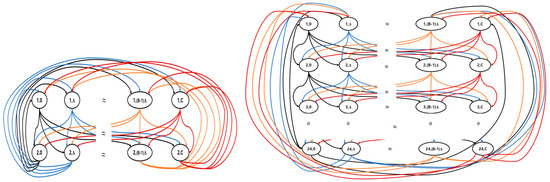
Figure 1. The examples of state space (T = 12 h (left), T = 1 h (right)).

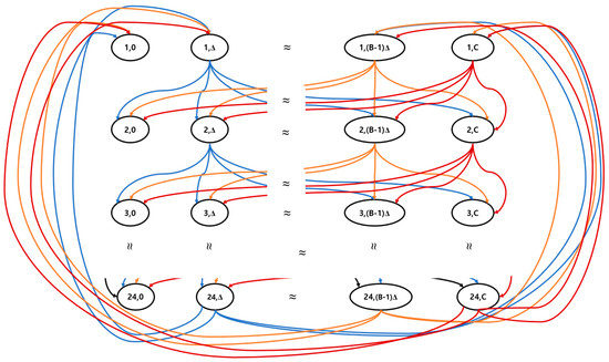
Figure 2. Absorbing Markov chain example (T = 1 h).

In [25], it is stated that, if the discrete time-homogeneous Markov chain is irreducible, then it is positive recurrent and periodic. There is a unique solution to the balance equations $\pi =\pi Q$ and $\sum _{\left(i,j\right)\in S}{\pi }_{\left(i,j\right)}=1,$ where $Q$ is a transition probability matrix (abovementioned), $\pi$ is a row vector representing the equilibrium probabilities. Each element ${\pi }_{\left(i,j\right)}$ in $\pi$, is the equilibrium probability that the Markov chain is in state (i,j). For example, ${\pi }_{\left(1,0\right)}$ represents the probability that the battery state is 0 at 1:00 a.m. if each hour is defined as a time index (T = 1 h). As such, our Markov chain model can be used to predict the distribution of battery state at each time point. Also, the following performance measures can be considered for capacity design of battery and PV resources of the system.

$$P\left[battery is empty\right]=1-Availability={{\displaystyle \sum }}_i{\pi }_{\left(i,0\right)},$$

(17)

$$P\left[battery is full\right]={{\displaystyle \sum }}_i{\pi }_{\left(i,C\right)}.$$

(18)

In [16], it is stated that “availabilities over 0.99999 or 5 nines are typically required for critical loads, such as conventional communication plants, whereas the U.S. grid availability is about 3 nines [26].” While most PV-energy storage systems are designed to meet this goal, there is another issue of PV resource size and energy storage system combination should be used to achieve the goal with minimal cost. Let $C_1$ and $C_2$ denote the operating cost of one unit of PV module and one unit of energy storage system per unit time, respectively. Then, the total operating cost of the system consisting of p units of PV modules and s units of the storage system is $p{C}_1+s{C}_2$. Since the availability requirement should be satisfied, the problem at hand becomes finding the values of p and s that satisfy the requirement $(\sum _i{\pi }_{\left(i,0\right)}<0.00001)$ at the lowest cost. Another measurement, the probability that the battery is full, can be used to check whether the storage system is oversized or not comparing to the capacity of PV modules. If the storage system is oversized, $\sum _i{\pi }_{\left(i,C\right)}$ decreases because there is less chance to fill the battery with the power produced by the PV module. Contrary, if the battery size is designed to be small, the power will fill the battery and the remaining power will be lost after the battery state reaches its capacity. In this case, the probability $\sum _i{\pi }_{\left(i,C\right)}$ has a large value.

Also, an Absorbing Markov chain technique can be employed to answer the following questions: (1) When a new battery is installed in the system, what is the average time it takes for the system’s battery state to go below a certain level? (2) If the system does not meet the load, when does the event occur?

By the definition in [25], state i is called an absorbing state when once the state is entered, it is impossible to leave. In other words, when a system state enters an absorbing state, it is stuck. A Markov chain that has at least one such state is called an Absorbing Markov chain.

In our Markov chain, we can define some states as absorbing states to answer the abovementioned questions. Let $U$ and $V$ denote sets of transient and absorbing states of the absorbing Markov chain, respectively. Suppose that we are interested in the average time until the battery runs out when a new battery is installed. Then,

$$U=\left\{\left(x,y\right)|\left(x,y\right)\in S,y>0\right\},$$

(19)

$$V=\left\{\left(x,y\right)|\left(x,y\right)\in S,y=0\right\}.$$

(20)

If we rearrange the states of Markov Chain in the order of transient states and absorbing states, the transition probability matrix, P, is

$$P=\left[\begin{array}{cc}{Q}^{\prime }& R\\ O_{\left|V\right|,\left|U\right|}& I_{\left|V\right|}\end{array}\right]$$

(21)

where $Q^{\prime }$ is a $\left|U\right|$-by-$\left|U\right|$ matrix, $R$ is a $\left|U\right|$-by-$\left|V\right|$ matrix, and $I_{\left|V\right|}$ is the $\left|V\right|$-by-$\left|V\right|$ identity matrix. Note that $\left|A\right|$ is the number of elements of set A.

$$Q^{\prime }=\left[\begin{array}{ccccccc}{O}_{B,B}& A_1^4& O_{B,B}& O_{B,B}& O_{B,B}& \cdots & O_{B,B}\\ O_{B,B}& O_{B,B}& A_2^4& O_{B,B}& O_{B,B}& \cdots & O_{B,B}\\ O_{B,B}& O_{B,B}& O_{B,B}& A_3^4& O_{B,B}& \cdots & O_{B,B}\\ ⋮& ⋮& ⋮& ⋮& ⋮& ⋮& ⋮\\ O_{B,B}& O_{B,B}& O_{B,B}& O_{B,B}& \cdots & O_{B,B}& A_{M-1}^4\\ A_M^4& O_{B,B}& O_{B,B}& O_{B,B}& \cdots & O_{B,B}& O_{B,B}\end{array}\right]$$

(22)

$$R=\left[\begin{array}{ccccccc}{O}_{B,1}& A_1^3& O_{B,1}& O_{B,1}& O_{B,1}& \cdots & O_{B,1}\\ O_{B,1}& O_{B,1}& A_2^3& O_{B,1}& O_{B,1}& \cdots & O_{B,1}\\ O_{B,1}& O_{B,1}& O_{B,1}& A_3^3& O_{B,1}& \cdots & O_{B,1}\\ ⋮& ⋮& ⋮& ⋮& ⋮& ⋮& ⋮\\ O_{B,1}& O_{B,1}& O_{B,1}& O_{B,1}& \cdots & O_{B,1}& A_{M-1}^3\\ A_M^3& O_{B,1}& O_{B,1}& O_{B,1}& \cdots & O_{B,1}& O_{B,1}\end{array}\right]$$

(23)

$$A_i^3=\left[\begin{array}{c}\sum _{j=-\infty }^{-1}{a}_{f\left(i\right)}\left(j\right)\\ \sum _{j=-\infty }^{-2}{a}_{f\left(i\right)}\left(j\right)\\ ⋮\\ \sum _{j=-\infty }^{-B+1}{a}_{f\left(i\right)}\left(j\right)\\ \sum _{j=-\infty }^{-B}{a}_{f\left(i\right)}\left(j\right)\end{array}\right]$$

(24)

$$A_i^4=\left[\begin{array}{ccccc}{a}_{f\left(i\right)}\left(0\right)& a_{f\left(i\right)}\left(1\right)& \cdots & a_{f\left(i\right)}(B-2)& \sum _{j=B-1}^{\infty }{a}_{f\left(i\right)}\left(j\right)\\ a_{f\left(i\right)}(-1)& a_{f\left(i\right)}\left(0\right)& \cdots & a_{f\left(i\right)}(B-3)& \sum _{j=B-2}^{\infty }{a}_{f\left(i\right)}\left(j\right)\\ ⋮& ⋮& ⋮& ⋮& ⋮\\ a_{f\left(i\right)}(-B+2)& a_{f\left(i\right)}(-B+3)& \cdots & a_{f\left(i\right)}\left(0\right)& \sum _{j=1}^{\infty }{a}_{f\left(i\right)}\left(j\right)\\ a_{f\left(i\right)}(-B+1)& a_{f\left(i\right)}(-B+2)& \cdots & a_{f\left(i\right)}(-1)& \sum _{j=0}^{\infty }{a}_{f\left(i\right)}\left(j\right)\end{array}\right]$$

(25)

Figure 2 illustrates an example of an Absorbing Markov chain model (T = 1 h). Note that no transition occurs from state (i,0) for all i. This is because the states are defined as absorbing states. The average time to run out of battery, $\mathsf{\alpha }$, can be calculated as follows:

$$\mathsf{\alpha }={\left[I_{\left|U\right|}-Q^{\prime }\right]}^{-1}e$$

(26)

where $e$ is a length-$\mathsf{\alpha }$ column vector whose entries are all 1. Note that $\alpha$ is a matrix consisting of a single column of $\left|U\right|$ elements. Each element in $\alpha$ represents the average time until the battery is exhausted when starting the system in the corresponding state. For example, the element corresponding to state (7,C) represents the average time until the battery is depleted when we install a new battery at 7:00 a.m. Thus, we can calculate the average time it takes to run out when a new battery is installed. Through a similar process, the absorbing state can be defined differently to calculate the time it takes for the battery to drop below a certain level.

3. Model Demonstration

The behavior of the proposed two models is simulated and the results are presented using MATLAB R2019b. The irradiance and load demand data sets used in the analysis are obtained at the Handong Global University Campus from March 2018 to February 2020, which were measured hourly. From the solar irradiance data, PV power generation is calculated as shown in Equation (27), considering the number ($N$), area ($A$), and efficiency $\left(\eta \right)$ of PV modules:

$$W\left(t\right)=N\times A\times \eta \times I\left(t\right), t=1 \mathrm{to} 24$$

(27)

Then, the net power of each hour, $X\left(t\right)$, can be calculated from the $W\left(t\right)$ and $L\left(t\right)$ in Equation (28) and the probability distributions of $X\left(t\right)$ are shown in Figure 3.

$$X\left(t\right)=W\left(t\right)-L\left(t\right) , t=1 \mathrm{to} 24$$

(28)

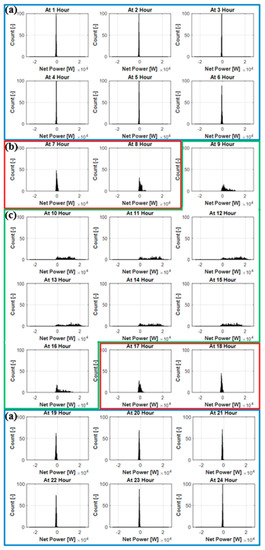
Figure 3. Hourly net power distribution. (a) 1:00 a.m. to 6:00 a.m. and 7:00 p.m. to 12:00 p.m. (b) 7:00 a.m. to 8:00 a.m. and 5:00 p.m. to 6:00 p.m. (c) 9:00 a.m. to 4:00 p.m.

Most previous research studies have calculated the net power based on the daily basis [17,18]. However, it may not explain the randomness of solar power generation and load demand within a day, which can significantly affect the availability. In Figure 3, hourly net power distributions are derived and the random characteristics within a day can be confirmed. As we can see in the figure, the net power distribution follows a different distribution every hour and this suggests that even though the average net power per day is sufficient, a power shortage may occur within a day. If the demand for power at a specific time exceeds the amount of power stored in battery + power generation at that time, a power shortage occurs. To consider those stochastic natures, this study assumes one-hour intervals for our Markov chain models. While the volatility may be better reflected in the model if we use a more specific unit of time (such as minutes or seconds), it can be a burden in data processing. For example, if the data interval is reduced to one minute, the data should be measured 60 times more often than the hourly based model, and the number of states in the Markov chain model will also increase. It increases the computational complexity to obtain the equilibrium probabilities [25].

Depending on the statistical values such as mean and variance values, Figure 3 shows that the net probability distribution can be classified into three groups: (1) 1:00 a.m. ~ 6:00 a.m. and 7:00 p.m. ~ 12:00 p.m., (2) 7:00 a.m. ~ 8:00 a.m. and 5:00 p.m. ~ 6:00 p.m., and (3) 9:00 a.m. ~ 4:00 p.m. Each group was divided into distributions of $D^1~D^3$, as previously mentioned in Section 2, in order to perform the simulation based on the proposed mathematical model. In $D^1 ~ D^3$, power difference between two adjacent states (Δ) is set with 125 kW, and each histogram is shown in Figure 4 with the mean values of −1056 kWh, −344 kWh, and 7610 kWh, respectively. Considering the visual features and the statistical values of the net distribution, it can be interpreted that the daily net power cannot represent the hourly measured random characteristic.

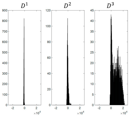
Figure 4. Histogram of $D^1 ~ D^3$ distribution.

Due to the nature of scheduled classes for each semester of the university, the campus power consumption data should be divided into semesters and break as well as weekdays and weekends. However, the average and variance values of the campus usage during the vacation and weekend shows only 9% differences with the average and variance of the entire power usage. Therefore, based on the statistical results, the whole data are used for obtaining enough sample data, regardless of vacation and weekend. When the proposed model is expanded to other applications, the prior data analysis can also be considered as an important factor influencing the results.

A. Performance of Embedded Markov Chain-Based Model

Since the model proposed in this paper is based on the power usage of the university campus, the optimal number of PV modules and ESS capacity is proposed based on the given target power supply availability of 3 nines. Figure 5 indicates the limiting probabilities according to number of PV modules and ESS capacity. For this experiment, the simulation was performed using the manufacturer of Hanwha with a PV module’s rated output of $150 \mathrm{W}$, size of $1.51 {\mathrm{m}}^2$, and efficiency of 0.153.

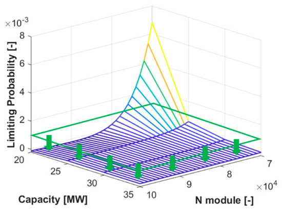
Figure 5. Limiting probability of Embedded Markov chain-based model.

In Figure 5, as the number of PV modules increases or the ESS capacity increases, the limiting probability is decreased. Also, the nonlinear characteristic can be checked through the sudden change in the limiting probability at specific points. In order to calculate the number of PV modules and ESS capacity required under a given limiting probability condition, the correlation of the three variables (limiting probabilities, PV module counts, ESS capacity numbers) are shown in Figure 6.

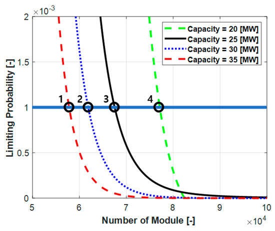
Figure 6. Points of Embedded Markov chain-based model when the limiting probability is 0.001.

In Figure 6, the four points represent the number of modules and ESS capacity when the target limiting probability is 0.001. When the ESS capacity increases, the number of modules has a great influence on the limiting probability. The values of each point are shown in Table 1.

Table 1. Value of each point in Figure 6.

Cases	ESS Capacity MWh	Number of Modules
1	35	57,800
2	30	61,870
3	25	67,510
4	20	77,140

The optimal number of PV modules and ESS capacity can be calculated from their prices at Figure 6. According to a report by Mirae Asset Daewoo Research 2020, “ESS connected to renewable energy” the ESS price is $251/kWh and the cost of installing a PV system including PV modules is $1.0/W. The results of calculating the price in the case of Table 1 are summarized in Table 2.

Table 2. Cost of each point in Figure 6.

Cases	ESS M$	PV System [M$]	Total [M$]
1	8.785	8.670	17.455
2	7.530	9.281	16.811
3	6.275	10.127	16.402
4	5.020	11.571	16.591

Therefore, Case 3 (ESS capacity: 25 MW, Number of Module: 67,510) can be proposed as the optimal point for satisfying 3-nine availability and having a minimum price.

B. Performance of Absorbing Markov Chain-Based Model.

When knowing the SOC of the ESS at a specific point, it is possible to predict a ESS’ lifetime until the battery is fully discharged based on the proposed absorbing Markov chain-based model. Considering the aging of the lithium-ion battery, it is considered as the time until the SOC of the battery remains more than 20% instead of complete discharge.

Here, we assume the initial battery SOC at 7:00 p.m. in four cases and estimate the time duration until the battery is discharged. The reason we assume the battery state at 7:00 p.m. as the initial state is that charging does not occur after 7:00 p.m. because the sun has set. As can be observed from the preceding data, no electricity is produced, only demand exists after sunset. Therefore, if the amount of power stored in the battery at sunset is insufficient, it may be difficult to meet the demand generated during the night. Using the absorption Markov chain model, it is possible to calculate the average time to discharge according to the state of the battery at sunset [25]. This simulation condition is based on the previous embedded Markov chain results (limiting probability: 3 nines, ESS capacity: 25 MW, Number of Modules: 67,510).

The higher the SOC of the battery is, as shown in Table 3, the more available the time. If the initial battery SOC is above 80%, there is no significant difference in available time. In addition, the initial battery SOC is important because overall availability varies significantly depending on the initial battery SOC.

Table 3. Available time according to initial battery SOC.

ESS SOC %	Available Time h
60	273.14
70	8407.88
80	20,287.48
90	22,082.46

4. Discussion

While various Markov chain models have been developed and employed as stochastic models to analyze the steady-state behavior of the energy storage systems, the variation caused by diurnal and the seasonal cycle is not considered in few researches. To include such variation into mathematical models, two Markov chain models are proposed. The Embedded Markov chain model enables us to calculate the probability that the state of ESS is at a certain level at a specific point of time. The variation is reflected in the transition probabilities of the model. The steady-state behavior of the battery state is fully characterized by the Embedded Markov chain model. The model can be used to calculate the optimal number of PV modules and ESS capacity satisfying a certain service level. Also, with the proposed Absorbing Markov chain model, the time duration until the energy system fails to supply power to loads can be estimated. The model can be used to calculate the average time duration until a new battery state becomes lower than a certain service level. To verify our model, we applied our model to the data of a university in Pohang, South Korea, from May 2018 to February 2020.

The results in this paper were evaluated with the price model received from the renewable energy evaluation agency, Mirae Asset Daewoo corporation. The corporation assessed the total cost of the PV system at $1/W for commercialized PV modules. This means that the price model represents the total installation cost of PV systems including PV modules, inverters, and protection circuits but it is regardless of the rated output and the size. Therefore, an approach that can evaluate the optimal PV modules size and ESS capacity which can satisfy the sustainable power supply availability of 3 nines (99.9%) has been made based on the price model. For example, the results when PV module (size of 2 ${\mathrm{m}}^2$ and the rated output 300 W) is applied to the proposed Markov chain model are shown in Table 4 and Table 5.

Table 4. Capacity sizing with new PV module applied.

Cases	ESS Capacity MWh	Number of Modules
1	35	47,600
2	30	53,530
3	25	62,700
4	20	75,300

Table 5. Cost with new PV module applied.

Cases	ESS M$	PV System M$	Total M$
1	8.785	15.708	24.493
2	7.530	17.665	25.195
3	6.275	20.691	26.966
4	5.020	24.849	29.869

It is expected that only half of the modules will be needed when comparing the results with the previous one of Hanwha’s PV module (rated output of $150 \mathrm{W}$, size of $1.51 {\mathrm{m}}^2$), because the rated output is doubled. However, the results in Table 4 and Table 5 show that while the number of modules decreased slightly, the total cost increased significantly for all cases compared to the results in Table 3 and Table 4. It can be interpreted that the design of PV installation corresponding to the environmental conditions is an important point since the PV modules’ outputs are depending on the variation of solar irradiation caused by diurnal and the seasonal cycle.

Our research can be further studied in various directions in the future. One direction is to obtain closed-form expressions for the equilibrium probabilities under the specific load and power generation patterns. The research scope in this paper is to calculate the probabilities numerically based on data. However, the closed-form expressions for the probabilities could provide additional insight into understanding the steady-state behavior. Moreover, it would be interesting to study the continuous-time state Markov process in Equation (2). In future studies, the application of the Markov decision process to existing Markov chains for control of the energy system should be studied. Especially, this application for battery electric vehicles and wind power plants will also be another important area to investigate.

References

- Riffonneau, Y.; Bacha, S.; Barruel, F.; Ploix, S. Optimal power flow management for grid connected PV systems with batteries. IEEE Trans. Sustain. Energy 2011, 2, 309–320. [Google Scholar] [CrossRef]
- El-Dein, M.S.; Kazerani, M.; Salama, M.M.A. Optimal photovoltaic array reconfiguration to reduce partial shading losses. IEEE Trans. Sustain. Energy 2012, 4, 145–153. [Google Scholar] [CrossRef]
- Dudley, B. “BP Statistical Review of World Energy 2019” BP Statistical Review. London, UK, June 2019. Available online: https://www.bp.com/content/dam/bp/business-sites/en/global/corporate/pdfs/energy-economics/statistical-review/bp-stats-review-2019-full-report.pdf (accessed on 21 January 2021).
- Touafek, K.; Haddadi, M.; Malek, A. Modeling and experimental validation of a new hybrid photovoltaic thermal collector. IEEE Trans. Energy Convers. 2011, 26, 176–183. [Google Scholar] [CrossRef]
- Abdelrazik, A.S.; Al-Sulaiman, F.A.; Saidur, R.; Ben-Mansour, R. A review on recent development for the design and packaging of hybrid photovoltaic/thermal (PV/T) solar systems. Renew. Sustain. Energy Rev. 2018, 95, 110–129. [Google Scholar] [CrossRef]
- Bathurst, G.N.; Strbac, G. Value of combining energy storage and wind in short-term energy and balancing markets. Elect. Power Syst. Res. 2003, 67, 1–8. [Google Scholar] [CrossRef]
- Kim, S.K.; Jeon, J.H.; Cho, C.H.; Ahn, J.B.; Kwon, S.H. Dynamic modeling and control of a grid-connected hybrid generation system with versatile power transfer. IEEE Trans. Ind. Electron. 2008, 55, 1677–1688. [Google Scholar] [CrossRef]
- Pardo, M.Á.; Manzano, J.; Valdes-Abellan, J.; Cobacho, R. Standalone direct pumping photovoltaic system or energy storage in batteries for supplying irrigation networks. Cost analysis. Sci. Total. Environ. 2019, 673, 821–830. [Google Scholar] [CrossRef]
- Achaibou, N.; Haddadi, M.; Malek, A. Modeling of lead acid batteries in PV systems. Energy Procedia 2012, 18, 538–544. [Google Scholar] [CrossRef]
- Knutel, B.; Pierzyńska, A.; Dębowski, M.; Bukowski, P.; Dyjakon, A. Assessment of Energy Storage from Photovoltaic Installations in Poland Using Batteries or Hydrogen. Energies 2020, 13, 4023. [Google Scholar] [CrossRef]
- Pardo, M.Á.; Fernández, H.; Jodar-Abellan, A. Converting a Water Pressurized Network in a Small Town into a Solar Power Water System. Energies 2020, 13, 4013. [Google Scholar] [CrossRef]
- Das, C.K.; Bass, O.; Kothapalli, G.; Mahmoud, T.S.; Habibi, D. Overview of energy storage systems in distribution networks: Placement, sizing, operation, and power quality. Renew. Sustain. Energy Rev. 2018, 91, 1205–1230. [Google Scholar] [CrossRef]
- Yang, Y.; Bremner, S.; Menictas, C.; Kay, M. Battery energy storage system size determination in renewable energy systems: A review. Renew. Sustain. Energy Rev. 2018, 91, 109–125. [Google Scholar] [CrossRef]
- Wong, L.A.; Ramachandaramurthy, V.K.; Taylor, P.; Ekanayake, J.B.; Walker, S.L.; Padmanaban, S. Review on the optimal placement, sizing and control of an energy storage system in the distribution network. J. Energy Storage 2019, 21, 489–504. [Google Scholar]
- Wu, L.; Wen, C.; Ren, H. Reliability evaluation of the solar power system based on the Markov chain method. Int. J. Energy Res. 2017, 41, 2509–2516. [Google Scholar] [CrossRef]
- Tao, L.; Ma, J.; Cheng, Y.; Noktehdan, A.; Chong, J.; Lu, C. A review of stochastic battery models and health management. Renew. Sustain. Energy Rev. 2017, 80, 716–732. [Google Scholar] [CrossRef]
- Kakimoto, N.; Matsumura, S.; Kobayashi, K.; Shoji, M. Two-state Markov model of solar radiation and consideration on storage size. IEEE Trans. Sustain. Energy 2013, 5, 171–181. [Google Scholar] [CrossRef]
- Song, J.; Krishnamurthy, V.; Kwasinski, A.; Sharma, R. Development of a Markov-chain-based energy storage model for power supply availability assessment of photovoltaic generation plants. IEEE Trans. Sustain. Energy 2012, 4, 491–500. [Google Scholar] [CrossRef]
- Kwasinski, A.; Krishnamurthy, V.; Song, J.; Sharma, R. Availability evaluation of micro-grids for resistant power supply during natural disasters. IEEE Trans. Smart Grid 2012, 3, 2007–2018. [Google Scholar] [CrossRef]
- Barton, J.P.; Infield, D.G. A probabilistic method for calculating the usefulness of a store with finite energy capacity for smoothing electricity generation from wind and solar power. J. Power Sources 2006, 162, 943–948. [Google Scholar] [CrossRef]
- Mulder, F.M. Implications of diurnal and seasonal variations in renewable energy generation for large scale energy storage. J. Renew. Sustain. Energy 2014, 6, 033105. [Google Scholar] [CrossRef]
- Li, M.; Allinson, D.; He, M. Seasonal variation in household electricity demand: A comparison of monitored and synthetic daily load profiles. Energy Build. 2018, 179, 292–300. [Google Scholar] [CrossRef]
- Liu, Y.; Wu, J. Multiple solutions of ordinary differential systems with min-max terms and applications to the fuzzy differential equations. Adv. Differ. Equ. 2015, 2015, 1–13. [Google Scholar] [CrossRef]
- Kalaba, R. On nonlinear differential equations, the maximum operation, and monotone convergence. J. Math. Mech. 1959, 8, 519–574. [Google Scholar] [CrossRef]
- Ross, S.M. “Markov Chains” in Stochastic Process, 2nd ed.; Wiley: New York, NY, USA, 1996. [Google Scholar]
- Robinson, D.G.; Arent, D.J.; Johnson, L. Impact of distributed energy resources on the reliability of critical telecommunications facilities. In Proceedings of the INTELEC 06-Twenty-Eighth International Telecommunications Energy Conference, Providence, RI, USA, 10–14 September 2006; pp. 1–7. [Google Scholar]
Publisher’s Note: MDPI stays neutral with regard to jurisdictional claims in published maps and institutional affiliations. |
© 2021 by the authors. Licensee MDPI, Basel, Switzerland. This article is an open access article distributed under the terms and conditions of the Creative Commons Attribution (CC BY) license (https://creativecommons.org/licenses/by/4.0/).